Symbolic Evaluation Graphs and Term Rewriting — A General Methodology for Analyzing Logic Programs ∗

(1)

Symbolic Evaluation Graphs and Term Rewriting — A General Methodology for Analyzing Logic Programs ^∗

J¨urgen Giesl

LuFG Informatik 2, RWTH Aachen University, Germany giesl@informatik.rwth-aachen.de

Thomas Str¨oder

LuFG Informatik 2, RWTH Aachen University, Germany stroeder@informatik.rwth-aachen.de

Peter Schneider-Kamp

Dept. of Mathematics and Computer Science, University of Southern Denmark

petersk@imada.sdu.dk

Fabian Emmes

LuFG Informatik 2, RWTH Aachen University, Germany

emmes@informatik.rwth-aachen.de

Carsten Fuhs

Dept. of Computer Science, University College London, United Kingdom

c.fuhs@cs.ucl.ac.uk

Abstract

There exist many powerful techniques to analyzeterminationand complexity of term rewrite systems (TRSs). Our goal is to use these techniques for the analysis of other programming languages as well. For instance, approaches to prove termination of definite logic programs by a transformation to TRSs have been studied for decades. However, a challenge is to handle languages with more complex evaluation strategies (such asProlog, where predicates like thecutinfluence the control flow). In this paper, we present a general methodology for the analysis of such programs. Here, the logic program is first transformed into asymbolic evaluation graph which represents all possible evaluations in a finite way.

Afterwards, different analyses can be performed on these graphs.

In particular, one can generate TRSs from such graphs and apply existing tools for termination or complexity analysis of TRSs to infer information on the termination or complexity of the original logic program.

Categories and Subject Descriptors D.1.6 [Programming Tech- niques]: Logic Programming; F.3.1 [Logics and Meanings of Pro- grams]: Specifying and Verifying and Reasoning about Programs—

Mechanical Verification; I.2.2 [Artificial Intelligence]: Automatic Programming—Automatic Analysis of Algorithms

General Terms Languages, Theory, Verification

Keywords Logic Programs, Prolog, Term Rewriting, Termina- tion, Complexity, Determinacy

∗Supported by the DFG under grant GI 274/5-3, the DFG Research Train- ing Group 1298 (AlgoSyn), and the Danish Council for Independent Re- search, Natural Sciences.

Permission to make digital or hard copies of all or part of this work for personal or classroom use is granted without fee provided that copies are not made or distributed for profit or commercial advantage and that copies bear this notice and the full citation on the first page. To copy otherwise, to republish, to post on servers or to redistribute to lists, requires prior specific permission and/or a fee.

PPDP’12, September 19–21, 2012, Leuven, Belgium.

Copyright c2012 ACM 978-1-4503-1522-7/12/09. . . $10.00

1. Introduction

We are concerned with analyzing “semantical” properties of logic programs, liketermination,complexity, anddeterminacy(i.e., the question whether all queries in a specific class succeed at most once). While there are techniques and tools that analyze logic pro- gramsdirectly, we present a generaltransformationalmethodology for such analyses. In this way, one can re-use existing powerful techniques and tools that have been developed forterm rewriting.

For well-moded definite logic programs, there are several trans- formations to TRSs such that termination of the TRS implies termination of the original logic program [33]. We extended these trans- formations to arbitrary definite programs in [35].

However,Prologprograms typically use thecutpredicate. To handle the non-trivial control flow induced by cuts, in [37] we introduced a pre-processing method where aPrologprogram is first transformed into asymbolic evaluation graph. (These graphs were inspired by related approaches to program optimization [38]

and were called “termination graphs” in [37].) Symbolic evaluation graphs also represent those aspects of the program that cannot eas- ily be expressed in term rewriting. We also developed similar approaches for other programming languages likeJavaandHaskell [7–9, 17]. ForProlog, the transformation from the program to the symbolic evaluation graph relies on a new “linear” operational semantics which we presented in [41]. From the symbolic evaluation graph, one can then generate a simpler program (without cuts) whose termination implies termination of the originalPrologpro- gram. In [37] we generated definite logic programs from the graph (whose termination could then be analyzed by transforming them further to TRSs, for example). In [40], we presented a more powerful approach which generates so-calleddependency triples[31, 36]

from the graph.

In the current paper, we show that the symbolic evaluation graph cannot only be used for termination analysis, but it is also very suitable as the basis for several other analyses, such as complexity or determinacy analysis. So symbolic evaluation graphs and term rewriting can be seen as a general methodology for the analysis of programming languages likeProlog.¹

1This methodology can also be used to analyze programs in other languages. For example, in [8] we used similar graphs not just for termination proofs, but also for disproving termination and for detecting NullPointerExceptions inJavaprograms.

(2)

After recapitulating the underlying operational semantics in Sect. 2, we introduce the symbolic evaluation graph in Sect. 3. To use this graph for different forms of program analysis, we present several new theorems which express the connection between the

“abstract evaluations” represented in the graph and the “concrete evaluations” of actual queries.

In Sect. 4, we present a new improved approach for termination analysis of logic programs, where one directly generatesterm rewrite systemsfrom the symbolic evaluation graph. This results in a substantially more powerful approach than [37]. Compared to [40], our new approach is considerably simpler and it allows us to applyanytool for termination of TRSs when analyzing the termination of logic programs. So one does not need tools that handle the (non-standard) notion of “dependency triples” anymore.

In Sect. 5 we show that symbolic evaluation graphs and the TRSs generated from the graphs can also be used in order to analyze thecomplexityof logic programs. Here, we rely on recent results which show how to adapt techniques for termination analysis of TRSs in order to prove asymptotic upper bounds for the runtime complexity of TRSs automatically.

Finally, Sect. 6 demonstrates that the symbolic evaluation graph can also be used to analyze whether a class of queries isdeter- ministic. Besides being interesting on its own, such a determinacy analysis is also needed in our new approach for complexity analysis of logic programs in Sect. 5.

We implemented all our contributions in our automated termination toolAProVE[15] and performed extensive experiments to compare our approaches with existing analysis techniques which work directly on logic programs. It turned out that our approaches for termination and complexity clearly outperform related existing techniques. For determinacy analysis, our approach can handle many examples where existing methods fail, but there are also many examples where the existing techniques are superior. Thus, here it would be promising to couple our approach with existing ones. All proofs can be found in [18].

2. Preliminaries and Operational Semantics of Prolog

See, e.g., [2] for the basics of logic programming. We label indi- vidual cuts to make their scope explicit. Thus, we use a signature Σcontaining{!m/0|m∈N}and all predicate and function symbols. As in the ISO standard forProlog[23], we do not distinguish between predicate and function symbols and just considerterms T(Σ,V)and no atoms.

Aqueryis a sequence of terms. LetQuery(Σ,V)denote the set of all queries, whereis the empty query. Aclauseis a pairh:-B where theheadhis a term and thebodyBis a query. IfBis empty, then we write just “h” instead of “h:-”. Alogic programPis a finite sequence of clauses.

We now briefly recapitulate our operational semantics from [41], which is equivalent to the ISO semantics in [23]. As shown in [41], both semantics yield the same answer substitutions, the same termination behavior, and the same complexity. The advantage of our semantics is that it is particularly suitable for an extension toclassesof queries, i.e., for the symbolic evaluation ofabstract states, cf. Sect. 3. This makes our semantics particularly well suited for analyzing logic programs.

Our semantics is given by a set of inference rules that operate onstates. Astatehas the form(G1 | . . . | Gn)where eachGi

is agoal. Here,G1 represents the current query and(G2 | . . . | Gn) represents the queries that have to be considered next. This backtrack information is contained in the state in order to describe the effect of cuts. Since each state contains all backtracking goals,

our semantics islinear(i.e., anevaluationwith these rules is just a sequence of states and not a search tree as in the ISO semantics).

Essentially, agoalis just a query, i.e., a sequence of terms. But to compute answer substitutions, a goal is labeled by a substitution which collects the unifiers used up to now. So if(t1, . . . , tk)is a query, then a goal has the form(t1, . . . , tk)θ for a substitution θ. In addition, a goal can also be labeled by a clause c, where (t1, . . . , tk)^c_θ means that the next resolution has to be performed with clausec. Moreover, a goal can also be ascope marker?mfor m∈N. This marker denotes the end of the scope of cuts!mlabeled withm. Whenever a cut!mis reached, all goals preceding?mare discarded.

Def. 1 shows the inference rules for the part ofPrologdefining definite logic programming and the cut. See [41] for the inference rules for fullProlog. Here,S and S⁰ are states and the queryQ may also be(then “(t, Q)” ist).

DEFINITION1 (Operational Semantics).

θ|S

S (SUC) (t, Q)^h_θ^:^-^B|S

(Bσ, Qσ)θσ|S (EVAL) ifmgu(t, h) =σ

?m|S

S (FAIL) (t, Q)^h:_θ ^-^B|S

S (BACKTRACK) ift6∼h (t, Q)θ|S

(t, Q)^c_θ¹^[!/!^m^]|. . .|(t, Q)^c_θ^a^[!/!^m^]|?m|S (CASE) wheretis no cut or variable,mis fresh, andSliceP(t) = (c1, . . . , ca)

(!m, Q)θ|S|?m|S⁰ Qθ|?m|S⁰ (CUT)

where S contains no

?m

(!m, Q)θ|S Qθ

(CUT) where S contains no

?m

The SUCrule is applicable if the first goal of our sequence could be proved. Then we backtrack to the next goal in the sequence.

FAIL means that for the currentm-th case analysis, there are no further backtracking possibilities. But the whole evaluation does not have to fail, since the stateSmay still contain further alternative goals which have to be examined.

To make the backtracking possibilities explicit, the resolution of a program clause with the first atomtof the current goal is split into two operations. The CASErule determines which clauses could be applied totby slicing the program according tot’s root symbol.

Here,SliceP(p(t1, . . . , tn))is the sequence of all program clauses

“h:-B” fromPwhereroot(h) =p/n. The variables in program clauses are renamed when this is necessary to ensure variable- disjointness with the states. Thus, CASEreplaces the current goal (t, Q)θby a goal labeled with the first such clause and adds copies of(t, Q)θ labeled by the other potentially applicable clauses as backtracking possibilities. Here, the top-down clause selection rule is taken into account. The cuts in these clauses are labeled by a fresh markm∈N(i.e.,c[!/!m]is the clausecwhere all cuts ! are replaced by!m), and?mis added at the end of the new backtracking goals to denote their scope.

EXAMPLE2. Consider the following logic program.

star(XS,[ ]):- !. (1)

star([ ],ZS):- !,eq(ZS,[ ]). (2) star(XS,ZS):- app(XS,YS,ZS),star(XS,YS).(3)

app([ ],YS,YS). (4)

app([X|XS],YS,[X|ZS]):- app(XS,YS,ZS). (5)

eq(X, X). (6)

Here,star(t1, t2)holds ifft2results from repeated concatenation of t1. So we havestar([1,2],[ ]),star([1,2],[1,2]),star([1,2],[1,2,

(3)

1,2]), etc. The cut in rule (2) is needed for termination of queries of the formstar([ ], t). For the querystar([1,2],[ ]), we obtain the following evaluation, where we omitted the labeling by substitutions for readability.

star([1,2],[ ]) `CASE

star([1,2],[ ])⁽¹⁰⁾|star([1,2],[ ])⁽²⁰⁾|star([1,2],[ ])⁽³⁾|?1 `EVAL

!1|star([1,2],[ ])⁽²⁰⁾|star([1,2],[ ])⁽³⁾|?1 `CUT

|?1 `SUC

?1 `FAIL ε So theCASErule results in a state which represents a case analysis where we first try to apply the star-clause (1). The state also contains the next backtracking goals, since when backtracking later on, we would use clauses (2) and (3). Here,(1⁰)denotes(1)[!/!1] and(2⁰)denotes(2)[!/!1].

For a goal(t,Q)^h_θ^:^-^B, iftunifies²with the headhof the program clause, we apply EVAL. This rule replacestby the bodyBof the clause and applies the mguσto the result. Moreover,σcontributes to the answer substitution, i.e., we replace the labelθbyθσ.

Iftdoes not unify withh (denoted “t 6∼ h”), we apply the BACKTRACKrule. Then,h:-Bcannot be used and we backtrack to the next goal in our backtracking sequence.

Finally, there are two CUTrules. The first rule removes all backtracking information on the levelmwhere the cut was introduced.

Since its scope is explicitly represented by!m and ?m, we have turned the cut into alocaloperation depending only on the current state. Note that?mmust not be deleted as the current goalQθcould still lead to another cut!m. The second CUTrule is used if?mis missing (e.g., if a cut!mis already in the initial query). We treat such states as if?mwere added at the end of the state.

For each queryQ, its correspondinginitial stateconsists of just (Q[!/!1])id(i.e., all cuts inQare labeled by a fresh number like 1 and the goal is labeled by the identity substitutionid). The query Q is terminatingif all evaluations starting in its corresponding initial state are finite. Our inference rules can also be used to define answer substitutions.

DEFINITION3 (Answer Substitution).LetSbe a state with a single goalQσ(which may additionally be labeled by a clausec). We say thatθis ananswer substitutionforSif there is an evaluation fromSto a state(^σθ|Ssuffix)for a (possibly empty) stateSsuffix

(i.e.,(^σθ|Ssuffix)is obtained by repeatedly applying rules from Def. 1 toS). Similarly,θis ananswer substitutionfor a query if it is an answer substitution for the query’s initial state.

3. From Prolog to Symbolic Evaluation Graphs

We now explain the construction ofsymbolic evaluation graphs which represent all evaluations of a logic program for a certain classof queries. While we already presented such graphs in [37], here we introduce a new formulation of the corresponding abstract inference rules which is suitable for generating TRSs afterwards.

Moreover, we present new theorems (Thm. 5, 8, and 10) which express the exact connection between abstract and concrete evaluations. These theorems will be used to prove the soundness of our analyses later on.

We consider classes of atomic queries described by ap/n∈Σ and amoding functionm: Σ×N→ {in,out}. Somdetermines which arguments of a symbol are “inputs”. The corresponding class of queries isQ^p_m = {p(t1, . . . , tn) | V(ti) = ∅for alliwith

2In this paper, we consider unification with occurs check. Our method could be extended to unification without occurs check, but we left this as future work since most programs do not rely on the absence or presence of the occurs check.

m(p, i) = in}. Here, “V(ti)” denotes the set of all variables occurring inti. So for the program of Ex. 2, we might regard the class of queriesQ^starm wherem(star,1) =m(star,2) =in. Thus, Q^starm ={star(t1, t2)|t1, t2are ground}.

To represent classes of queries, we regardabstractstates that stand for sets of concrete states. Instead of “ordinary” variablesN, abstract states use abstract variablesA={T1, T2, . . .}represent- ing fixed, but arbitrary terms (i.e.,V=N ] A).

To obtain concrete states from an abstract one, we use concretizations. A concretization is a substitutionγ which replaces all abstract variables by concrete terms, i.e.,Dom(γ) = Aand V(Range(γ))⊆ N. To determine by which terms an abstract variable may be instantiated, we add a knowledge baseKB = (G,U) to each state, where G ⊆ A and U ⊆ T(Σ,V)× T(Σ,V).

The variables inGmay only be instantiated by ground terms, i.e., V(Range(γ|_G)) =∅. Here, “γ|_G” denotes the restriction ofγtoG, i.e.,γ|_G(X) =γ(X)forX ∈ Gandγ|_G(X) =XforX∈ V \ G.

A pair(t, t⁰) ∈ U means that we are restricted to concretizations γwheretγ 6∼ t⁰γ, i.e.,tand t⁰ must not be unifiable afterγ is applied. Then we say thatγis a concretizationw.r.t.KB.

Thus, an abstract state has the form(S;KB). Here,S has the form(G1 | . . . | Gn)where theGiare goals over the signature Σand the abstract variablesA(i.e., they do not contain variables fromN). In contrast to [37], we again label all goals (except scope markers) by substitutionsθ:V → T(Σ,A)in order to store which substitutions were applied during an evaluation. These substitution labels will be necessary for the synthesis of TRSs in Sect. 4.

The notion ofconcretizationcan also be used for states. A (concrete) stateS⁰is a concretization of(S;KB)if there exists a con- cretizationγ w.r.t.KB such thatS⁰ results fromSγ by replacing the substitution labels of its goals by arbitrary (possibly different) substitutionsθ : N → T(Σ,N). To ease readability, we often write “Sγ” to denote an arbitrary concretization of(S;KB). Let CON(S;KB)denote the set of all concretizations of an abstract state(S;KB).

For a classQ^pmwithp/n, now theinitial stateis(p(T1, . . . , Tn)id,(G,∅)), whereGcontains allTiwithm(p, i) =in.

We now adapt the inference rules of Def. 1 to abstract states.

The rules SUC, FAIL, CUT, and CASEdo not change the knowledge base and are straightforward to adapt. In Def. 1, we determined which of the rules EVAL and BACKTRACK to apply by trying to unify the first termt with the head h of the corresponding clause. But in the abstract case we might need to apply EVAL

for some concretizations and BACKTRACKfor others. The abstract BACKTRACKrule in Def. 4 can be used iftγdoes not unify with hforanyconcretizationγ. Otherwise,tγunifies withhforsome concretizationsγ, but possibly not forothers. Thus, the abstract EVALrule has two successor states to combine both the concrete EVALand the concrete BACKTRACKrule. Consequently, we now obtain symbolic evaluation trees instead of sequences.

DEFINITION4 (Abstract Inference Rules).

(θ|S);KB

S;KB (SUC) ((!m, Q)θ|S|?m|S⁰);KB

(Qθ|?m|S⁰);KB (CUT)whereS contains no?m

(?m|S);KB

S;KB (FAIL) ((!m, Q)_θ|S);KB

Qθ;KB (CUT)where S contains no?m

((t, Q)θ|S);KB

((t, Q)^c_θ¹^[!/!^m^]|. . .|(t, Q)^c_θ^a^[!/!^m^]|?m|S);KB (CASE) wheretis no cut or variable,mis fresh,SliceP(t) = (c1, . . . , ca)

(4)

((t, Q)^h_θ^:^-^B|S);KB

S;KB (BACKTRACK)

if there is no concretiza- tionγw.r.t.KBsuch that tγ∼h.

((t, Q)^h:_θ ^-^B|S); (G,U)

((Bσ, Qσ)θσ|S⁰); (G⁰,Uσ|_G) S; (G,U ∪ {(t, h)})(EVAL) ifmgu(t, h) = σ. W.l.o.g.,V(Range(σ))only contains fresh abstract variables andDom(σ)contains all previously occurring variables. More- over,G⁰=A(Range(σ|_G))andS⁰results fromSby applying the substi- tutionσ|_Gto its goals and by composingσ|_Gwith the substitution labels of its goals.

To handle “sharing” effects correctly [37], w.l.o.g. we assume thatmgu(t, h) = σrenames all occurring variables to fresh abstract variables in EVAL. The knowledge base is updated differently for the successors corresponding to the concrete EVALand BACK-

TRACKrule. For all concretizations corresponding to the second successor of EVAL, the concretization oftdoes not unify withh.

Hence, here we add(t, h)toU.

Now consider concretizations γ where tγ and h unify, i.e., these concretizations γ correspond to the first successor of the EVALrule. Then for anyT ∈ G,T γis a ground instance ofT σ.

Hence, we replace allT ∈ GbyT σ, i.e., we applyσ|_GtoS. The new setG⁰ of variables that may only be instantiated by ground terms are the abstract variables occurring inRange(σ|_G)(denoted

“A(Range(σ|_G))”). As before,t is replaced by the instantiated clause bodyBand the previous substitution labelθ is composed with the mguσ(yieldingθσ).

Thm. 5 states that any concrete evaluation with Def. 1 can also be simulated with the abstract rules of Def. 4.

THEOREM5 (Soundness of Abstract Rules).Let (S;KB) be an abstract state with a concretization Sγ ∈ CON(S;KB), and letSnext be the successor ofSγaccording to the operational semantics in Def. 1. Then the abstract state(S;KB)has a successor(S⁰;KB⁰)according to an inference rule from Def. 4 such that Snext ∈ CON(S⁰;KB⁰).

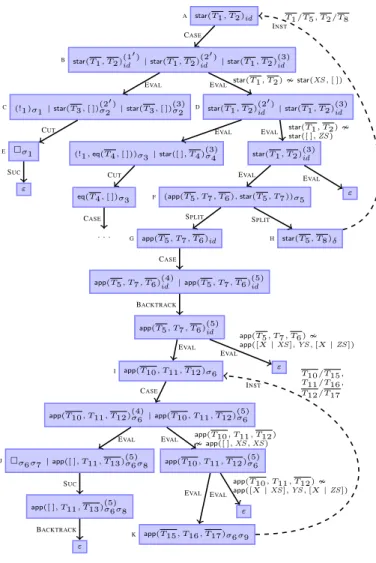
As an example, consider the program from Ex. 2 and the class of queriesQ^starm. The corresponding initial state is(star(T1, T2)id; ({T1, T2},∅)). Asymbolic evaluationstarting with this stateAis depicted in Fig. 6. The nodes of such a symbolic evaluation graph are states and each step from a node to its children is done by an inference rule. To save space, we omitted the knowledge base from the states(S; (G,U)). Instead, we overlined all variables contained inGand labeled those edges where new information is added toU.

The child ofAisBwith(star(T1, T2)⁽¹_id⁰⁾ |star(T1, T2)⁽²_id⁰⁾ | star(T1, T2)⁽³⁾_id |?1). In Fig. 6 we simplified the states by removing markers?mthat occur at the end of a state. This is possible, since applying the first CUT rule to a state ending in?m corresponds to applying the second CUT rule to the same state without?m. Moreover,(1⁰)and(2⁰)again abbreviate(1)[!/!1]and(2)[!/!1].

InB,(1⁰)is used for the next evaluation. EVALyields two successors: InC,σ1 =mgu(star(T1, T2),star(XS,[ ])) ={T1/T3, XS/T3, T2/[ ]}leads to((!1)σ₁ |star(T3,[ ])⁽²σ₂⁰⁾|star(T3,[ ])⁽³⁾σ₂).

Here,σ2=σ1|_{T

1,T2}. In the second successorDofB, we add the informationstar(T1, T2) 6∼ star(XS,[ ])toU (thus, we labeled the edge fromBtoDaccordingly).

Unfortunately, even for terminating queries, in general the rules of Def. 4 yield an infinite tree. The reason is that there is no bound on the size of terms represented by the abstract variables and hence, the abstract EVALrule can be applied infinitely often. To represent all possible evaluations in a finite way, we need additional inference rules to obtain finite symbolic evaluation graphs instead of infinite trees.

star(T1, T2 )id A

star(T1, T2 )(10)

id |star(T1, T2 )(20)

id |star(T1, T2 )(3) id B

CASE

(!1)σ1|star(T3,[ ])(20)

σ2 |star(T3,[ ])(3) σ2 C

EVAL

star(T1, T2 )(20)

id |star(T1, T2 )(3) id D

EVAL star(T1, T2 )star(XS,[ ])

σ1 E

CUT

(!1,eq(T4,[ ]))σ3|star([ ], T4 )(3) σ4

EVAL

star(T1, T2 )(3) id EVAL star(T1, T2 )

star([ ],ZS)

ε SUC

eq(T4,[ ])σ3 CUT

(app(T5, T7, T6 ),star(T5, T7 ))σ5 F

EVAL

ε EVAL

. . . CASE

app(T5, T7, T6 )id G

SPLIT

star(T5, T8 )δ H

SPLIT INST

T1/T5, T2/T8

app(T5, T7, T6 )(4)

id |app(T5, T7, T6 )(5) id CASE

app(T5, T7, T6 )(5) id BACKTRACK

app(T10, T11, T12 )σ6 I

EVAL

ε EVAL

app(T5, T7, T6 ) app([X|XS],YS,[X|ZS])

app(T10, T11, T12 )(4)

σ6 |app(T10, T11, T12 )(5) σ6 CASE

σ6σ7|app([ ], T11, T13 )(5) σ6σ8 J

EVAL

app(T10, T11, T12 )(5) σ6 EVAL app(T10, T11, T12 )

app([ ],XS,XS)

app([ ], T11, T13 )(5) σ6σ8 SUC

app(T15, T16, T17 )σ6σ9 K

EVAL

INST

T10/T15, T11/T16, T12/T17

ε EVAL

app(T10, T11, T12 ) app([X|XS],YS,[X|ZS])

ε BACKTRACK

Figure 6. Symbolic Evaluation Graph for Ex. 2

To this end, we use an additional INSTrule which allows us to connect the current state(S;KB)with a previous state(S⁰;KB⁰), provided that the current state is an instance of the previous state.

In other words, every concretization of(S;KB)must be a concretization of(S⁰;KB⁰). More precisely, there must be a matching substitutionµsuch thatS⁰µ =S up to the substitutions used for labeling goals inS⁰ andS. These substitution labels do not have to be taken into account here, since we will not generate rewrite rules from paths that traverse INSTedges in Sect. 4. Moreover, for KB⁰ = (G⁰,U⁰)andKB = (G,U),G⁰ andGmust be the same (moduloµ) and all constraints fromU⁰must occur inU(moduloµ).

Then we say thatµisassociatedto(S;KB)and label the resulting INSTedge withµ. For example, in Fig. 6,µ={T1/T5, T2/T8}is associated toHand the edge fromHtoAis labeled withµ. We only define the INSTrule for states containing a single goal. As indicated by our experiments, this is no severe restriction in practice.³

3In [37] and in our implementation, we use an additional inference rule to split up sequences of goals, but we omitted it here for readability. Adding this rule allows us to construct a symbolic evaluation graph for each program and query.

(5)

DEFINITION7 (Abstract Rules: INST).

S; (G,U) S⁰; (G⁰,U⁰)(INST)

if S = Qθ and S⁰ = Q⁰_θ0 orS = Q^c_θandS⁰ =Q^0c_θ0 for some non-empty queriesQandQ⁰, such that there is aµ withDom(µ) ⊆ A,V(Range(µ)) ⊆ A,Q=Q⁰µ,G=S

T∈G⁰V(T µ), and U⁰µ⊆ U.

Thm. 8 states that every concrete state represented by an INST

node is also represented by its successor.

THEOREM8 (Soundness of INST).Let (S;KB) be an abstract state, let(S⁰;KB⁰)be its successor according to the INSTrule, and letµbe associated to(S;KB). IfSγ ∈ CON(S;KB), then forγ⁰=µγwe haveS⁰γ⁰∈ CON(S⁰;KB⁰).

Moreover, we also need a SPLITinference rule to split a state ((t, Q)θ;KB)into(tid;KB)and((Qδ)δ;KB⁰), whereδapprox- imates the answer substitutions fort. Such a SPLITis often needed to make the INSTrule applicable. We say thatδ isassociatedto ((t, Q)θ;KB). The previous substitution labelθdoes not have to be taken into account here, since we will not generate rewrite rules from paths that traverse SPLITnodes in Sect. 4. Thus, we can re- set the substitution labelθtoidin the first successor of the SPLIT

node and store the associated substitutionδin the substitution label of the second successor. Similar to the INSTrule, we only define the SPLITrule for states containing a single goal.

DEFINITION9 (Abstract Rules: SPLIT).

(t, Q)θ; (G,U)

tid; (G,U) (Qδ)δ; (G⁰,Uδ) ^(S^PLIT⁾

where δ replaces all previously occurring variables fromA\Gby fresh abstract variables andG⁰ = G ∪ NextG(t,G)δ.

Here,NextG is defined as follows. We assume that we have a groundness analysisfunction GroundP : Σ×2^N → 2^N, see, e.g., [22]. If p/n ∈ Σ and {i1, . . . , im} ⊆ {1, . . . , n}, then GroundP(p,{i1, . . . , im}) ={j1, . . . , jk}means that any que- ryp(t1, . . . , tn) ∈ T(Σ,N) whereti₁, . . . , ti_m are ground only has answer substitutions θ where tj₁θ, . . . , tj_kθ are ground.

So GroundP approximates which positions of p will become ground if the “input” positionsi1, . . . , imare ground. Now ift= p(t1, . . . , tn) ∈ T(Σ,A)is an abstract term whereti₁, . . . , ti_m

become ground in every concretization (i.e., all their variables are fromG), thenNextG(t,G)returns all variables intthat will be made ground by every answer substitution for any concretization oft. Thus,NextG(t,G)contains the variables oftj₁, . . . , tj_k. So formally

NextG(p(t1, . . . , tn),G) =[

j∈Ground_P(p,{i|V(t_i)⊆G})V(tj).

Hence, in the second successor of the SPLITrule, the variables in NextG(t,G)can be added to the groundness setG. Since these variables were renamed byδ, we extendGbyNextG(t,G)δ.

For instance, in Fig. 6, we split the query app(T5, T7, T6), star(T5, T7)in stateF. Thus, the first successor ofFisapp(T5, T7, T6)in stateG. By groundness analysis, we infer that every success- ful evaluation ofapp(T5, T7, T6)instantiatesT7by ground terms, i.e.,GroundP(app,{1,3}) ={1,2,3}. Thus, forG ={T5, T6}, we haveNextG(app(T5, T7, T6),G) =V(T5)∪V(T7)∪V(T6) = {T5, T7, T6}. So in the second successorHofF, we use the substitution δ(T7) = T8 and extend the groundness set G ofF by NextG(app(T5, T7, T6),G)δ = {T5, T8, T6}. Thus, T8 is also overlined in Fig. 6.

Thm. 10 shows the soundness of SPLIT. Suppose that we apply the SPLITrule to((t, Q)θ;KB), which yields(tid;KB)and

((Qδ)δ;KB⁰). Any evaluation of a concrete state (tγ,Qγ) ∈ CON((t, Q)θ;KB) consists of parts where one evaluates tγ (yielding some answer substitutionθ⁰) and of parts where one evaluatesQγθ⁰. Clearly, those parts which correspond to evaluations oftγcan be simulated by the left successor of the SPLIT

node (sincetγ ∈ CON(tid;KB)). Thm. 10 states that the parts of the overall evaluation which correspond to evaluations ofQγθ⁰ can be simulated by the right successor of the SPLIT node (i.e., Qγθ⁰∈ CON((Qδ)δ;KB⁰)).

THEOREM10 (Soundness of SPLIT).Let((t,Q)θ;KB)be an abstract state and let(tid;KB)and((Qδ)δ;KB⁰)be its successors according to theSPLITrule. Let(tγ, Qγ)∈ CON((t, Q)θ;KB) and let θ⁰ be an answer substitution of (tγ)id. Then we have Qγθ⁰∈ CON((Qδ)δ;KB⁰).

We define symbolic evaluation graphs as a subclass of the graphs obtained by the rules of Def. 4, 7, and 9. They must not have any cycles consisting only of INSTedges, as this would lead to trivially non-terminating TRSs. Moreover, their only leaves may be nodes where no inference rule is applicable anymore (i.e., the graphs must be “fully expanded”). The graph in Fig. 6 is indeed a symbolic evaluation graph.

DEFINITION11 (Symbolic Evaluation Graph). A finite graph built from an initial state using Def. 4, 7, and 9 is asymbolic evaluation graph(or “evaluation graph” for short) iff there is no cycle consisting only ofINSTedges and all leaves are of the form(ε;KB).⁴

4. From Symbolic Evaluation Graphs to TRSs – Termination Analysis

Now our goal is to show termination of all concrete states represented by the graph’s initial state. To this end, we synthesize a TRS from the symbolic evaluation graph. This TRS has the following property: if there is an evaluation from a concretization of one state to a concretization of another state which may be crucial for termination, then there is a corresponding rewrite sequence w.r.t. the TRS. Then automated tools for termination analysis of TRSs can be used to show termination of the synthesized TRS and this implies termination of the original logic program. See, e.g., [13, 16, 43] for an overview of techniques for automatically proving termination of TRSs.

For the basics of term rewriting, we refer to [6]. Aterm rewrite systemRis a finite set of rules`→rwhere` /∈ V andV(r)⊆ V(`). The rewrite relationt→Rt⁰for two termstandt⁰holds iff there is an`→r ∈ R, a positionpos, and a substitutionσsuch that`σ=t|posandt⁰=t[rσ]pos. Here,t|posis the subterm oftat positionposandt[rσ]posresults from replacing the subtermt|pos

at positionposintby the termrσ. The rewrite step isinnermost (denotedt→ⁱ Rt⁰) iff no proper subterm of`σcan be rewritten.

To obtain a TRS from an evaluation graph Gr, we encode the states as terms. For each states = (S; (G,U)), we use two fresh function symbolsfsⁱⁿ and fs^out. The arguments of fsⁱⁿ are the variables inG(which represent ground terms). The arguments off_s^outare those remaining abstract variables which will be made ground by every answer substitution for any concretization ofs.

They are again determined by groundness analysis [22]. Formally, the encoding of states is done by two functionsencⁱⁿ andenc^out.

For instance, for the state Fin Fig. 6, we obtainencⁱⁿ(F) = fFⁱⁿ(T5, T6)(asG ={T5, T6}in F) andenc^out(F) = fF^out(T7).

The reason is that ifγinstantiatesT5andT6by ground terms, then

4The application of inference rules to abstract states is not deterministic. In our proverAProVE, we implemented a heuristic [39] to generate symbolic evaluation graphs automatically which turned out to be very suitable for subsequent analyses in our empirical evaluations.

(6)

every answer substitution of(app(T5, T7, T6)γ,star(T5, T7)γ)in- stantiatesT7γto a ground term as well.

For an INSTnode likeHwith associated substitutionµwe do not introduce fresh function symbols, but use the function symbol of its (more general) successor instead. So we take the terms resulting from its successorAand applyµto them. In other words, encⁱⁿ(H) = encⁱⁿ(A)µ = fAⁱⁿ(T1, T2)µ = fAⁱⁿ(T5, T8) and encôut(H) =encôut(A)µ=fAôutµ=fAôut.

In the following, for an evaluation graphGrand an inference rule RULE, Rule(Gr) denotes all nodes ofGr to which RULE

was applied. LetSucci(s) denote the i-th child of node s and Succi(Rule(Gr))denotes the set ofi-th children of all nodes from Rule(Gr).

DEFINITION12 (Encoding States as Terms).Letsbe an abstract state with a single goal (i.e.,s= ((t1, . . . , tk)θ; (G,U))), and let V(s) =V(t1)∪. . .∪ V(tk). We define

encⁱⁿ(s) =

(encⁱⁿ(Succ1(s))µ,ifs∈Inst(Gr)whereµis associated tos

fsⁱⁿ(Gⁱⁿ(s)), otherwise, whereGⁱⁿ(s) =G ∩ V(s)

enc^out(s) =







enc^out(Succ1(s))µ, ifs ∈ Inst(Gr) whereµis associated tos

fsôut(Gôut(s)), otherwise, where Gôut(s) = NextG((t₁, ..., t_k),G)\ G

Here, we extendedNextGto work also on queries:

NextG((t1, . . . , tk),G) = NextG(t1,G)∪

NextG( (t2, . . . , t_k),NextG(t1,G) ).

So to computeNextG((t1, . . . , tk),G)for a query (t1, . . . , tk), in the beginning we only know that the variables inG represent ground terms. Then we compute the variablesNextG(t1,G)which are made ground by all answer substitutions for concretizations of t1. Next, we computeNextG(t2,NextG(t1,G))which are made ground by all answer substitutions for concretizations oft2, etc.

Now we encode the paths ofGras rewrite rules. However, we only considerconnection pathsofGr, which suffice to analyze termination. Connection paths are non-empty paths that start in the root node of the graph or in a successor of an INSTor SPLITnode, provided that these states are not INSTor SPLITnodes themselves.

So the start states in our example areA,G, andI. Moreover, connection paths end in an INST, SPLIT, or SUCnode or in the successor of an INSTnode, while not traversing INSTor SPLITnodes or successors of INSTnodes in between. So in our example, the end states areA,E,F,H,I,J,K, but apart fromEandJ, connection paths may not traverse any of these end nodes in between.

Thus, we have connection paths fromAtoE,AtoF,GtoI,Ito

J, andItoK. These paths cover all ways through the graph except for INST edges (which are covered by the encoding of states to terms), for SPLITedges (which we consider later in Def. 15), and for graph parts without cycles or SUCnodes (which cannot cause non-termination).

DEFINITION13 (Connection Path).A pathπ=s1. . . skis acon- nection pathof an evaluation graphGriffk >1and

•s1∈ {root(Gr)} ∪Succ1(Inst(Gr)∪Split(Gr))∪ Succ2(Split(Gr))

•sk∈Inst(Gr)∪Split(Gr)∪Suc(Gr)∪Succ1(Inst(Gr))

•for all1≤j < k,sj∈/Inst(Gr)∪Split(Gr)

•for all1< j < k,sj∈/Succ1(Inst(Gr))

For a connection pathπ, letσπrepresent the unifiers that were applied along the path. These unifiers can be determined by “com- paring” the substitution labels of the first and the last state of the path (i.e., the goal inπ’s first state has a substitution labelθand

the first goal ofπ’s last state is labeled byθσπ). So for the connection pathπfromAtoFwe haveσπ = σ5, whereσ5(T1) = T5 and σ5(T2) = T6. For this path, we generate rewrite rules which evaluate the instantiated input termencⁱⁿ(A)σπfor the start nodeAto its output termenc^out(A)σπif the input termencⁱⁿ(F) for the end node can be evaluated to its output termenc^out(F).

So we getencⁱⁿ(A)σπ → uA,F(encⁱⁿ(F),V(encⁱⁿ(A)σπ) )and uA,F(enc^out(F),V(encⁱⁿ(A)σπ) ) → enc^out(A)σπ for a fresh function symboluA,F. In our example, this yields

fAⁱⁿ(T5, T6)→uA,F(fFⁱⁿ(T5, T6), T5, T6) (7) uA,F(fFôut(T7), T5, T6)→fAôut (8) However, for connection pathsπ⁰like the one fromAtoEwhich end in a SUCnode, the resulting rewrite rule directly evaluates the instantiated input termencⁱⁿ(A)σπ⁰for the start nodeAto its output termencôut(A)σπ⁰. So we obtain

fAⁱⁿ(T3,[ ])→fA^out (9) DEFINITION14 (Rules for Connection Paths).Letπbe a connection paths1. . . skin a symbolic evaluation graph. Let the (only) goal ins1be labeled by the substitutionθand let the first goal in skbe labeled by the substitutionθ σπ. Ifsk ∈Suc(Gr), then we defineConnectionRules(π) ={encⁱⁿ(s1)σπ→enc^out(s1)σπ}.

Otherwise,ConnectionRules(π) =

{encⁱⁿ(s1)σπ → us₁,s_k(encⁱⁿ(sk),V(encⁱⁿ(s1)σπ) ), us₁,s_k(enc^out(sk),V(encⁱⁿ(s1)σπ) ) → enc^out(s1)σπ}, whereus₁,s_kis a fresh function symbol.

In addition to the rules for connection paths, we also need rewrite rules to simulate the evaluation of SPLIT nodes like F. Let δ be the substitution associated to F (i.e., δ represents the answer substitution ofF’s first successorG). Then the SPLITnodeF

succeeds (i.e.,encⁱⁿ(F)δcan be evaluated toencôut(F)δ) if both successorsGandHsucceed (i.e.,encⁱⁿ(G)δ can be evaluated to encôut(G)δ andencⁱⁿ(H)can be evaluated to encôut(H)). Note thatencⁱⁿ(F)andencⁱⁿ(G)only contain “input” arguments (i.e., abstract variables fromG) and thus,δdoes not modify them. Hence, encⁱⁿ(F)δ=encⁱⁿ(F)andencⁱⁿ(G)δ=encⁱⁿ(G). So we obtain fFⁱⁿ(T5, T6)→uF,G(fGⁱⁿ(T5, T6), T5, T6) (10) uF,G(fGôut(T8), T5, T6)→uG,H(fAⁱⁿ(T5, T8), T5, T6, T8) (11) uG,H(fAôut, T5, T6, T8)→fFôut(T8) (12) DEFINITION15 (Rules for Split,R(Gr)).Let s ∈ Split(Gr), s1=Succ1(s), ands2=Succ2(s). Moreover, letδbe the substitution associated tos. ThenSplitRules(s) =

{encⁱⁿ(s) → us,s₁(encⁱⁿ(s1),V(encⁱⁿ(s)) ), us,s₁(enc^out(s1)δ,V(encⁱⁿ(s)) ) →

us₁,s₂(encⁱⁿ(s2),V(encⁱⁿ(s))∪ V(encôut(s1)δ) ), us₁,s₂(encôut(s2),V(encⁱⁿ(s))∪V(encôut(s1)δ))→encôut(s)δ}

R(Gr)consists ofConnectionRules(π)for all connection paths πand ofSplitRules(s)for allSPLITnodessofGr.

For the graphGrof Fig. 6, the resulting TRSR(Gr)consists of (7) – (12) and the connection rules (13), (14) for the path from

Gto I(where σ6(T5) = [T9 | T10], σ6(T7) = T11, σ6(T6) = [T9|T12]), the rules (15), (16) forItoK(whereσ9(T10) = [T14| T15], σ9(T11) =T16, σ9(T12) = [T14|T17]), and (17) forIto J

(whereσ8=σ7|_{T

10,T₁₂}withσ8(T10) = [ ], σ8(T12) =T13).