Field theory of disordered bosons

Feldtheorie ungeordneter Bosonen

Diplomarbeit

von Sebastian E. Schmittner

Betreuer: Prof. Dr. Martin R. Zirnbauer

Universität zu Köln

Institut für theoretische Physik

1 Introduction 1

1.1 Motivation . . . 1

1.2 Outline . . . 3

1.3 German introduction . . . 4

2 Model 7 2.1 The setting . . . 7

2.1.1 The Hamiltonian . . . 7

2.1.2 Modelling the spatial structure . . . 10

2.1.3 Restrictions . . . 12

2.2 The resolvent operator . . . 14

2.2.1 Definition . . . 14

2.2.2 Gaussian integrals . . . 15

2.2.3 Superbosonisation . . . 17

3 Field theory 25 3.1 Approximations . . . 25

3.1.1 Continuum limit . . . 25

3.1.2 Saddle point equations . . . 28

3.1.3 Action landscape . . . 29

3.1.4 Fluctuations . . . 35

3.1.5 Consistency check . . . 38

3.2 Coordinate free description . . . 39

3.2.1 Symmetric super-spaces . . . 39

3.2.2 Super-groups . . . 40

3.2.3 Involutions and subgroups . . . 41

3.2.4 Bundle decomposition . . . 43

3.2.5 Differential super-geometry . . . 47

3.2.6 The action . . . 49

4 Dimension Zero 53 4.1 Bulk scaling . . . 53

4.2 Spectral edges . . . 55

4.3 Edge scaling . . . 56

4.3.1 Saddle point method reviewed . . . 56

4.3.2 Density of frequencies . . . 58

5 Discussion 61

A Appendix 65

A.1 Explicit forms of the super-spaces . . . 65

A.1.1 Lie super-algebras . . . 65

A.1.2 Root space decomposition . . . 66

A.1.3 Lie super-groups . . . 67

A.2 Saddle point . . . 69

A.3 Grassmann integral . . . 69

A.4 Residue . . . 70

A.5 Invariant measure . . . 71

1.1 Motivation

Quantum field theories have in many instances be successfully applied to qualitatively and quantitatively understand fundamental questions in condensed matter physics.

Effective field theories emerge in many different settings and have, in the form of non- linearσ-models, provided profound insight into the physics of disordered systems, for an example see [Efe99].

The goal of this diploma thesis is to develop a field theory, for a specific class of disordered bosonic systems, in order to study, whether disordered bosons generically have universal statistical properties, similar to fermions.¹

For fermionic systems the universality question is well understood. There exist ten families of symmetry classes, as explained by Zirnbauer et. al. in [Zir98, AZ97, HHZ04]. These classes determine the statistics, i.e. the probability distributions of the correlation functions, of low-energy excitations of ergodic systems.

For bosons, one might doubt on physical grounds whether there is universal be- haviour at low energies at all. In condensed matter, bosonic modes typically arise as Goldstone modes, where low energy usually means long wavelength. But long wavelength modes are insensitive to spatially uncorrelated weak disorder, which gets effectively averaged out on the scale of the wavelength. This argument does, how- ever, not apply in general. Long wavelength modes might be suppressed or forbidden by boundary conditions, the disorder might be strong, in real systems the disorder will never be spatially uncorrelated and, generally speaking, the multi particle ground state might be such that low lying excitations have a comparatively short wavelength.

Anyhow, as soon as low lying excitations of a wavelength comparable to the length scale of the disorder exist, it seems reasonable to assume that their behaviour will be largely determined by symmetries, rather than by microscopic details, just as in the fermionic case. In fact, hints to universal behaviour were found in [GC02] and also [GA04] for systems where the bosonic excitations are not of Goldstone type.

In order to shed some light on those questions, the general idea is to investigate a quadratic model, which should be thought of as being the lowest order approximation of a system of small oscillations around the (interacting) many particle ground state.

Physical examples of such systems where the fluctuations quantise as bosons are

• vibrations of amorphous solids, see e.g. [GKK89],

• oscillations of the superfluid density of Bose-Einstein condensates,

1As such this thesis is part of the research project C3 ‘The universality question for disordered low-frequency bosons’ within the SFB/TR12.

• excitations of Bose glasses, see e.g. [FWGF89],

• photons in an inhomogeneous optical medium,

• spin waves in disordered magnets, see e.g. [WW77],

• and normal modes of pinned charge density waves, see e.g. [GS88].

Now, if disordered bosons show system independent statistical features, the evident question is whether the bosonic universality classes are different from the fermionic ones. For fermions, the classification in terms of symmetric spaces is a largely alge- braical one, which happens in a complexified setting before compact or non-compact real forms are specified. Hence one can rightly state that all effective bosonic non-linear σ-models are already classified within the ten fold way together with the fermionic ones.

And indeed, in the system studied in [LSZ06], well known universal GUE statistics were found in the bulk and Lück finds GOE statistics in [Lü09], both for systems of disordered bosons.

But for bosons non-linearσ-models are not everything. A subtle point about non- interacting, i.e. quadratic, bosonic systems is stability. One single particle state of negative energy for a bosonic system immediately leads to an unbounded many particle Hamiltonian. For fermionic systems, a finite number of such single particle states is of no concern, due to the Pauli principle. This important difference leads to the well studied Gaussian ensembles not providing feasible distributions of bosonic Hamiltonians. If, however, more complicated probability distributions are taken into account, one has to be prepared to face a more complicated effective model than a pure non-linear σ-model in the end. In this sense, an interesting question is whether bosonic systems if they show universal behaviour lead to novel universality classes.

A hint to those might be the unusual density of states near zero energy that was found in [LSZ06] or [GC02] and [GA04]. On physical grounds, one can expect the commutation relations of bosons to have important effects at low frequencies, which fits to the observations of [GC02] and [GA05].

In this thesis, we will develop and study a specific model, which is the next step after the work of Lück, Sommers and Zirnbauer, [LSZ06], towards a more realistic description of a disordered system of bosonic degrees of freedom. As in [LSZ06], our model is still purely random, i.e. there is no limit of an underlying pure system and we also stay with a model without global symmetries, such as time reversal or charge conjugation. But we turn from the homogeneous, zero-dimensional model to a spatially extended one and implement the physically important feature of locality. Furthermore, we add an additional parameter to tune the number of modes per volume. In particular we can hereby enforce a macroscopical number of zero modes. The goal is to study the density of states of the new model and therefore to develop an effective field theory.

Throughout we will pay special attention to the region near zero frequency and watch out for unusual, possibly universal features.

1.2 Outline

In chapter 2 we will introduce the model to be studied in this thesis. A copy of the zero-dimensional model which was solved in [LSZ06] is placed on each vertex of a graph, which defines the spatial structure. Then we add random interactions in between neighbouring vertices. Note that, although we will specialise to a regular square lattice in chapter 3 to develop a continuum field theory, the results of chapter 2 are more general. One could also put the model on a more complicated graph to emulate, e.g., a real system consisting of a few isolated grains or dots and only allow for interactions in between specific sites. Or, a quasi one- or two-dimensional system, which is extended in one but finite in another direction, might be constructed. Anyway, no such system is considered here. As we are looking for universal features, rather than trying to model a concrete real system, we will consider the simplest spatial structure.

Furthermore, the resolvent operator is introduced in section 2.2 and super-symmetry methods are applied in order to average out the disorder, leading to the final step of superbosonisation and hence to the exact formulation of the effective model as a lattice field theory in equation (2.24).

Chapter 3 hosts the main part of this thesis. Here we will perform a continuum limit and carefully study a saddle point approximation, justified by taking the limit of a large number N of degrees of freedom per volume. Deriving the saddle point equa- tions, considering the reachability of all possible saddle points for various parameter configurations and expanding the fluctuations to quadratic order will take the sections 3.1.2 to 3.1.4.

In section 3.2 various notions from the differential geometry of Riemannian sym- metric (super-) spaces will be introduced. Finally, we will propose a general form of the effective action, describing the resolvent operator, in section 3.2.6 and determine the coefficients therein from the coordinate based calculations in 3.1.4. This concludes the derivation of the field theory as advertised in the title.

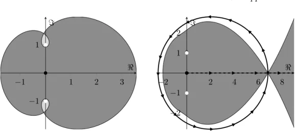
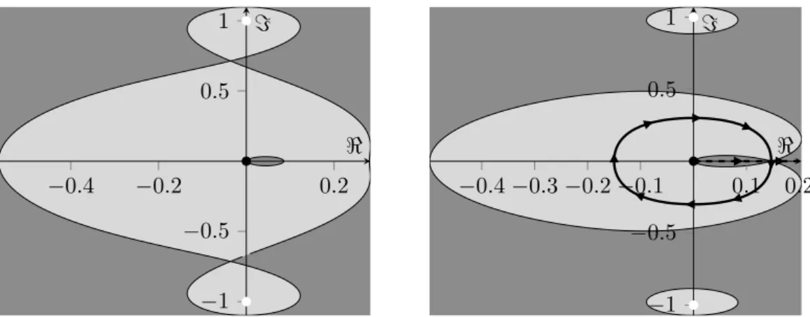
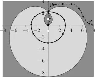
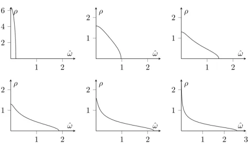
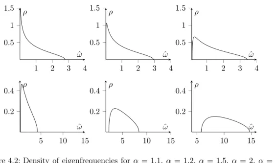
After this is finished, we turn our attention back to the zero dimensional case in chapter 4. Here we will explicitly calculate the density of states to first order in _N¹ and compare to [LSZ06]. We allow a parameter which already exists in [LSZ06] to vary in a much larger range. This parameter tunes the distribution for the random coupling constants, which physically affects e.g. the number of zero modes in the model. The significance of this parameter becomes visible in the figures 4.1 and 4.2.

For a summary of the results see section 5.

1.3 Einleitung

Quantenfeldtheorien sind ein probates und erfolgreiches Instrument zur qualitativen und quantitativen Beschreibung, Untersuchung und Lösung fundamentaler Probleme im Rahmen der Physik kondensierter Materie. Effektive Feldtheorien, insbesondere in der Form nicht linearer σ-Modelle, haben in vielen Fällen zu tiefen Einsichten in die Physik ungeordneter Systeme geführt, ein Beispiel hierführ ist das Buch von Efetov [Efe99].

Das Ziel dieser Arbeit ist es eine Feldtheorie für eine bestimmte Klasse ungeordneter bosonischer Systeme zu entwickeln und zu untersuchen, ob bosonische ungeordnete Systeme universelle Eigenschaften haben, wie das bei fermionischen Systemen der Fall ist.²

Die universellen Eigenschaften ungeordneter fermionischer Systeme sind ausgiebig untersucht worden und es wurde insgesamt ein gutes Verständnis erreicht. Es gibt zehn Universalitätsklassen wie von Zirnbauer u.a. in [Zir98, AZ97, HHZ04] beschrieben. Die Zugehörigkeit zu einer dieser Klassen bestimmt die Statistik, d.h. die Wahrscheinlich- keitsverteilung der Korrelationsfunktionen, der niederenergetischen Anregungen ergo- discher Systeme.

Es ist nicht von vornherein klar, ob auch Bosonen universelle Eigenschaften bei nied- rigen Energien zeigen. Typischerweise treten bosonische Anregungen in der Festkör- perphysik in Form von Goldstone-Moden, für die niedrige Energie große Wellenlänge bedeutet, auf. Solche langwelligen Moden sind unempfindlich gegenüber schwacher, räumlich unkorrelierter Unordnung, da diese auf der Skala der Wellenlänge effektiv ge- mittelt wird. Nun gibt es aber auch eine Vielzahl von Systemen auf die dieses Argument nicht zutrifft, zum Beispiel wenn die Anregungen elementar bosonisch sind, z.B. Pho- tonen, wenn langwellige Anregungen durch z.B. Randbedingungen unterdrückt werden oder wenn die Unordnung hinreichend stark und oder räumlich korreliert ist, wobei zu- mindest letzteres in realen Systemen immer zu einem gewissen Grad der Fall sein wird.

Und die thermodynamische Intuition lehrt, sobald die niedrig energetischen Anregun- gen hinreichend stark von Unordnung beeinflusst werden, sollten ihre Eigenschaften eher durch die Symmetrien des Systems bestimmt werden als durch mikroskopische Details. Diese grundlegende Anschauung trifft auf Bosonen ebenso zu wie auf Fer- mionen und in der Tat wurden in [GC02] und [GA04] Hinweise auf ein universelles Verhalten bosonischer Systeme gefunden.

Um nun die Frage nach der Universalität für Bosonen systematisch zu untersuchen betrachten wir Systeme mit Hamilton Operatoren quadratischer Ordnung. Diese soll- ten als erste Näherung an reale, wechselwirkende Systeme verstanden werden, d.h. als effektive Theorien kleiner Schwingungen um einen stabilen Vielteilchen-Grundzustand.

Physikalische Beispiele solcher Systeme, bei denen die Anregungen als Bosonen quan- tisiert sind, wären

• Vibrationsmoden amorpher Festkörper, z.B. [GKK89],

2In diesem Sinne gliedert sich diese Arbeit in das Forschungsprojekt C3 ‘The universality question for disordered low-frequency bosons’ des SFB/TR12 ein.

• Oszillationen der Superflüssigkeitsdichte von Bose-Einstein-Kondensaten,

• Anregungen von Bose-Gläsern, z.B. [FWGF89],

• Photonen in inhomogenen optischen Medien,

• Spinwellen in ungeordneten Magneten, z.B. [WW77],

• und Normalmoden von Ladungsdichtewellen, z.B. [GS88].

Falls bosonische Systeme nun universelle Eigenschaften zeigen stellt sich die Fra- ge, ob diese in ähnlicher Art wie die fermionischen klassifiziert werden können und ob sie sich sogar in die schon bekannten Symmetrieklassen einfügen, oder ob es zur Beschreibung bosonischer Systeme neuer Symmetrieklassen bedarf. Da die Klassifizie- rung fermionischer Systeme mittels symmetrischer Räume im wesentlichen algebraisch ist könnte man nun annehmen, dass der von Zirnbauer u.a. beschriebene ‘ten fold way’

auch die bosonischen Systeme mit einschließt. In der Tat wurde in [LSZ06] gezeigt, dass die n-Punkt Funktionen für das Modell auf dem diese Arbeit aufbaut, gerade die des gausschen unitären Ensembles sind. In [Lü09] wurden Charakteristika des ortho- gonalen Ensembles beobachtet.

Im allgemeinen muss man aber davon ausgehen, dass Systeme ungeordneter Boso- nen nicht ohne weiteres auf reine nicht lineare σ-Modelle abgebildet werden können.

Ein wichtiger Punkt hierbei ist Stabilität des Grundzustandes um den entwickelt wird.

Hat der zugrundeliegende Einteilchen-Hamiltonoperator auch nur einen negativen Ei- genwert, so ist das Spektrum des Vielteilchen-Operators unweigerlich nach unten hin unbeschränkt, da kein Pauli-Prinzip wie bei Fermionen den Besetzungszahloperator beschränkt. Daher eignen sich gaussche Ensemble mit unabhängig identisch verteilten Matrixeinträgen des Hamiltonians grundsätzlich nicht zur Beschreibung bosonischer Probleme. Daher ist die Frage nach neuen Universalitätsklassen nicht eine Frage nach möglichen neuen Zielräumen für nicht lineare σ-Modelle. Diese sind vollständig klas- sifiziert. Vielmehr lautet die Frage, ob und wie die Klasse der effektiven Feldtheorien erweitert werden muss. Hinweise auf solche neuen Klassen könnten die ungewöhnliche Zustandsdichten sein, die in [LSZ06] oder auch [GC02] und [GA04] gefunden wurden.

Falls solche neuen Klassen zu neuartigen universellen Wahrscheinlichverteilungen füh- ren, so sollten diese am ehesten bei niedrigen Energien zu beobachten sein, was zu den Beobachtungen in [GC02] und [GA05] passen würde.

In dieser Arbeit wird ein spezielles Modell ungeordneter Bosonen entwickelt und un- tersucht werden, dass eine Weiterentwicklung des von Lück, Sommers und Zirnbauer, [LSZ06], gelösten Problems darstellt. Das hier betrachtete Modell ist weiterhin rein zufällig, d.h. es gibt keinen Grenzfall eines deterministischen Systems. In diesem Sinne könnte man von einem Grenzwert unendlich starker Unordnung sprechen. Weiterhin werden nach wie vor keine globalen Symmetrien, wie etwa Zeitumkehrsymmetrie, be- trachtet. Aber das neue Modell ist in so fern realistischer, als das nun räumliche Aus- dehnung in Betracht gezogen wird und der Hamiltonoperator nur lokal wirkt. Weiterhin gibt es in unserem Modell einen zusätzlichen Parameter, d.h. wir erweitern die Fami- lie der Wahrscheinlichkeitsverteilungen. Physikalisch bedeutet dies insbesondere, dass

Modelle mit einer makroskopischen Anzahl an Nullmoden in Betracht gezogen werden können. Das Ziel ist es, ein effektives Modell zur Beschreibung der Zustandsdichte zu entwickeln und insbesondere auf möglicherweise neuartige statistische Eigenschaften im Sinne der oben gestellten Universalitätsfrage zu untersuchen.

In this chapter we derive a lattice field theory. All derivations should be reasonably rigorous and, apart from the last step of superbosonisation for which we refer to [LSZ07], self contained.

2.1 The setting

We extend the bosonic random matrix ensemble considered in [LSZ06] and [Lü09], chapter 3, by adding spatial structure. Therefore, we will first review the general structure of a quadratic bosonic Hamiltonian in 2.1.1 and then define what we mean by spatial structure in 2.1.2 and describe the consequences for the ensemble of feasible Hamiltonians in 2.1.3.

Independently, an additional parameterα will be introduced into the model which can be tuned to enforce a macroscopical number of zero modes in all systems of the ensemble. For the case where all neighboring modes are coupled, α can be related to the parameter¹ k, the power of a factor of Det(h) in the probability density. See section 2.1.3, in particular the equations (2.8) and (2.9) for further details.

Depending on the physical system under consideration, e.g. phonons in a randomly distorted lattice, it might be unclear why one should want to have a macroscopical number of zero modes. But one should keep in mind that the pure random model, which will be build in this thesis, is not supposed to be ultimately realistic. In a subsequent step in the development of a complete picture of random bosonic systems, one should add a deterministic part to the model to get closer to physically relevant systems. In such a situation the zero modes of the random model will get mixed with the deterministic modes and thus would not remain at zero. However, for the pure random model itself, the zero modes have a positive effect, in so far, as the density of states becomes more realistic. This will be discussed in detail in section 4.

2.1.1 A generic quadratic Hamiltonian

A quadratic Hamiltonian frequently arises when one linearises the equations of mo- tion of a given system around a stable fixed point. We will now spell out what this stability means for the Hamiltonian, i.e. specify which kind of disorder is feasible for maintaining stable systems. The positivity constraint arising will be explained from the classical as well as from the quantum point of view. In any case, an isolated sys- tem can only be an idealisation of a system, which is weakly coupled to some sort of

1Note that our parameterkwas calledlin [Lü09].

environment. This idealisation has to break down for thermodynamic reasons, as soon as it is possible for the system to go to arbitrarily low energies. This is the case for a system of classical or bosonic quantum particles if there is a single particle state with negative energy. Note that, due to the Pauli principle, this is no problem for fermionic systems, where a finite number of single particle states of negative energy does not spoil thermodynamics.

As the theory developed in this thesis applies to bosonic quantum mechanical as well as classical systems, we will now introduce both viewpoints.

Classical Model

Let {Qi} denote the set of N canonical position variables with conjugate momenta {P_i}. I.e. Q and P form a canonical coordinate system for the 2N-dimensional symplectic phase space such that the symplectic form readsJ =dQ_i∧dP_i.

The most general quadratic Hamilton function is

H=Q_iA_ijQ_j+Q_iB_ijP_j+P_iC_ijQ_j+P_iD_ijP_j

=

Q^T P^T A B C D

! Q P

!

with Q^T := (Q₁, Q₂, . . . , Q_N), similarly for P^T, and A, B, C, D are N ×N matrices.

We have A =A^T, D=D^T and B =C^T and all matrix entries in the reals, because classical observables are commuting and real valued. Throughout,()^T will denote the usual matrix transpose. The important positivity constraint mentioned above is now simply a demand on

h:= A B C D

!

=h^T to be positive semidefinite.

We stress again that this positivity is what makes the classical and bosonic random matrix problems harder to handle than the fermionic ones, because we cannot simply choose some i.i.d. Gaussian measure for the independent matrix elements ofhto define our ensemble.

Another way to see why positivity is needed is that the truncation of the expansion of H at quadratic order is only sensible at a local minimum x = (Q₀, P₀) of H, i.e.

dH

_x = 0 and the Hessian

h= Hess(H) x

being positive definite. Negative eigenvalues of h would correspond to unstable di- rections, hence the system would leave the range of applicability of the quadratic expansion and one would then have to include higher order terms, e.g. in a next step proceed to a Ginsburg Landau type model.

After considering the energy, let us now have a look at the equations of motion²

−J Q˙ P˙

!

=h Q P

!

where J = 0 1_N

−1_N 0

!

(2.1) We are looking for a stable fixed point of the linearised differential equation x˙ = Xx with X = Jh. Physically speaking, as there is no damping, i.e. no energy dissipation mechanism, we will not find an attractive fixed point. Or, more formally, X = −JX^TJ⁻¹ ∈ sp(2N) is in the symplectic Lie algebra, which implies Det(λ1− X) = Det(λ1+X), i.e. all eigenvalues come in pairs, ±λ. Therefore demanding the fixed point to be stable, i.e. <(λ)≤0for all eigenvalues, means that they actually all have to be purely imaginary, λ=±˙ıω.

Having settled this reality constraint, we now come to positivity in the more formal picture. For a thermodynamic description to make sense, the action needs to be bounded from below in order for the partition function to exist. This leads to the additional constraint, which is best phrased in a geometric picture. Here positivity of the eigenfrequencies ω means that we have to restrict the domain of feasible random matricesX to a cone within the symplectic Lie algebra

D_X = (

X =g 0 ω

−ω 0

!

g⁻¹ |ω= diag(ω₁, . . . , ω_N), ω_i∈R⁺, g∈Sp(R^2N) )

whereSp(R^2N) =

g|gJg^T =J denotes the real symplectic group. Note that

U⁻¹ 0 ω

−ω 0

!

U = ˙ı −ω 0

0 ω

!

for U := √1 2

1_N 1_N

−˙ı1_N ı1˙ _N

!

∈U(2N)

i.e. this choice of D_X indeed guarantees thatX is diagonalisable with all eigenvalues purely imaginary.

To see thatD_X is also well chosen with respect to the positivity constraint, we write the Hamiltonian,h=J⁻¹X, in the new basis given by the basis changeg.³

H=

Q^T P^T

g^T h g Q P

!

=X

i

ω_i

P˜_i²+ ˜Q²_i

Hence positivity of the ωi physically means positive mass and spring constant of the harmonic oscillator modes. A negative mass term would lead to an unbounded spec- trum {P

in_iω_i|n_i ∈N}, which leads to e^−βH being non-integrable and hence the partition function would be ill defined.

2We use the same symbol for the symplectic form and its matrix as long as there is no ambiguity about the basis.

3g∈Sp(R^2N)⇔g^T∈Sp(R^2N)

Bosonic model

As usual we go from the classical to the quantum system by changing the Lie algebra representation from Poisson brackets to −˙ı times the commutator, but we keep the symbols{Qi}for the bosonic ‘position’ operators with conjugate momentum operators {P_i}. I.e.

[Q_i, P_j] = ˙ıδ_i,j [Q_i, Q_j] = [P_i, P_j] = 0 whereı˙:=√

−1. The most general quadratic Hamiltonian now formally looks exactly the same as before.

H= Q^T, P^T A B C D

! Q P

!

A, B, C, D are N ×N matrices and we have A =A^T,D =D^T by the commutation relations. To ensure Hermiticity of H we also need that B = C^† and A, B, C, D all real, so we get the same constituents for the matrixhas in the classical setting above.

Now we can view the positivity constraint from yet another perspective. Again we diagonalise the symmetric bilinear form h by using the same symplectic⁴ g as above. Now also the unitary matrix U from above will be recognised, namely as the transformation to creation and annihilation operators a^(†) = ^√1₂( ˜Q±ı˙P˜) as usual.

Applying both transformations leads to

U^Tg^T h gU = 0 ω ω 0

!

and hence to the standard quantum harmonic oscillator H =

a, a^† 0 ω ω 0

! a a^†

!

=X

i

ω_i(a^†_ia_i+a_ia^†_i)

where the ω_i are twice the standard frequencies, as in the classical case. And again we see that it is absolutely necessary to demand positivity of the ωi. We iterate that unlike in the fermionic case, where the particle number operator is bounded (Pauli principle), a single particle eigenstate with negative energy for a bosonic operator leads immediately to an unbounded operator on Fock space.

2.1.2 Modelling the spatial structure The underlying graph G

Throughout, we will denote the graph which defines the underlying spatial structure byG= (V, E)whereV is the (finite) set of vertices andE⊂(V ×V)/{(i, j)∼(j, i)}

4Whilst gbeing a symplectic transformation was most natural in the classical phase space, in the quantum setting the reader might be more used to this group of transformations being called

‘canonical’ and the preservation of the commutation relations under basis change with g being emphasised.

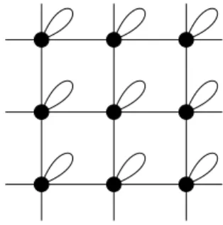
the set of undirected edges. We use the convention (i, i) ∈/ E, such thatE describes the actual spatial structure. But for the construction of the model we will mainly use Er :=E∪ {(i, i) ∈ V ×V} which can be visualised by an extra edge per vertex, see Figure 2.1.

Figure 2.1: Visualisation of the two-dimensional square lattice with an extra edge per site.

Although the considerations in this work apply, to a certain extent, to any kind of graph, we will mostly think of a d-dimensional cubic lattice with periodic boundary in the following. We denote the length of the sides of the cube (counting in number of vertices) by Lsuch that|V|=L^d and |E_r|=|E|+|V|=|V|(d+ 1).

Furthermore, fori∈V and e= (i, j) ∈Er we introduce the convenient ‘adjacency operator’ @e:={i, j} and @i:={f ∈E_r | ∃k∈V :f = (i, k)}. Instead of e∈ @i we will just write e@i.

Vector spaces on top of G

We equip the symplectic phase space with a spatial structure as follows:

At each sitei∈V we have a symplectic vector spaceS_i with symplectic formJ_i to model the local degrees of freedom. For simplicity we assume all Si to have the same dimension2N. The full phase space of the system is given by

S =M

i∈V

S_i

with the corresponding symplectic form J =L

i∈V J_i. We denote the canonical pro- jections by π_i^S :SSi.

Additionally we introduce auxiliary Euclidean vector spaces for each edge, again all with the same dimension ∀_e∈ErO_e'R^M and a total Euclidean space

O =M

e∈E

O_e

with canonical projections π_e^O : S S_e. Those will be used to model the random interactions in between neighbouring grains by e ∈ E and random couplings within the grains, i, by (i, i)∈E_R.

2.1.3 Restrictions on the Hamiltonian

The matrix h defining the characteristic frequencies as in 2.1.1 has not only to be positive, but additionally we require it to reflect the spatial structure imposed by the underlying graph.

h∈S:=n

h∈End(S)|h=h^T positive semidefinite and X

(i,j)∈E^r

π_i^S◦h◦π^S_j =ho

Note that the last condition can equivalently be written as π_i^S◦h◦π^S_j 6= 0⇒(i, j)∈E_r

and further that we only demand semidefiniteness, i.e. we also include the boundary of our cone and pass to D_X. In fact, later on we will see that only models which explicitly enforce a macroscopical number of zero modes have a finite, non vanishing density of eigenfrequencies near ω= 0 for d= 0.

Implementing the restrictions

To get our hands on a probability measure forh, we first decomposeh=l^Tl. Thereby, instead of demandinghto be symmetric positive semidefinite, we only need to requirel to be real. Secondly, to implement the spatial structure, we use the auxiliary Euclidean vector spaces on the edges, as introduced in 2.1.2. We define the following space of linear mappings

L:=

(

l:S−−−→

linear O|l=X

ei∈V@i

π_e^O◦l◦π^S_i )

(2.2)

Note the important summation constraint e@i which means that l(S_i) ⊂ L

e@iO_e and l^T(O_e)⊂L

i@eS_i. Therefore we get a well defined mapping φ:L→S

l7→h=l^Tl

The rest of this section will be spend on investigating the properties of φ. First, by diagonalising

g l^Tl g^T = diag(λ₁, . . . , λ_2N|V|)

with someg in the big orthogonal groupO(R^2N|V|), we see thatφ(L) contains regular elements if and only if

M|Er| ≥2N|V|

⇔ M ≥2N |V|

|E_r| = 2N d+ 1

(2.3)

where the last equality holds for the d-dimensional cubic lattice. This inequality motivates the introduction of the constant

α:= (d+ 1)M 2N +O

1 N

(2.4) where we anticipate that we will only needαup to terms of orderO _N¹

in the sequell.

α gets physical meaning by rephrasing the above observation: Our ensemble contains systems without zero modes as soon as α ≥1. In this case the probability of having zero modes is actually zero.⁵

Note, however, that O(R^2N|V|) does not respect the spatial structure and φ will in general not be surjective onto S. This can be seen by comparing dimensions

dim(L) = 2NM ·(2|E|+|V|) dim(S) = 2N(2N+ 1)

2 |V|+ (2N)²|E| (2.5) which means that φcan only be surjective for at least

M ≥ 2N+ 1 2

|V|

2|E|+|V|+ 2N |E|

2|E|+|V| =N + 1 4d+ 2 i.e. α≥ ^d+1₂ .

To get a more accurate estimate, one can easily see that the differentialdφ l0 at l₀ =M

v∈V

diag(1, . . . ,1) :S_v →O_(v,v)

is surjective if and only if M ≥ 2N. This means that only for α ≥ d+ 1 really all modes in neighbouring grains are coupled almost surely.

Choosing a family of probability measures

Using the implementation of the restrictions from the last section, the question of what would be a natural, or at least tractable, measure on the space of Hamiltonians of interest given by S can now be traced back to defining a ‘good’ measure on Land then pushing this forward withφ.

As explained in [Lü09], chapter 3.2, it is not possible to choose a measure like e^−Tr(Jh)2, which is invariant under the full symplectic symmetry group, because Sp is non-compact. Instead, as in [Lü09], we will consider a one-parameter family of measures which is invariant under the maximal compact subgroupU of Sp.

On the level ofl it is very natural to consider the Gaussian measure

dµ(l)∝e^−12Tr(lTl)dl (2.6)

5Strictly speaking, forα= 1theO`₁

N

´terms matter, even in the largeN limit, as can be seen in (2.3). However, forα≥1a realisation does almost surely not containmacroscopically many zero modes.

wheredlis the flat measures onL. This measure is in fact invariant under the product of unitary and orthogonal groups Q

i∈V U(Si)×Q

e∈E^rO(Oe), acting by

l7→hlg^T (2.7)

with h∈Q

e∈E^rO(Oe) andg∈Q

i∈V U(Si)whereU(Si)⊂Sp(Si) is understood.

If the differential dφ has full rank, i.e. α ≥ d+ 1, this measure can be pushed forward to

dµk(h) =φ∗(dµ(l))∝e^−12TrhDet(h)^kdh (2.8) where dh is the flat measure on the subset φ(L)⊂S. Otherwise the push forward of dµ(l)will be concentrated on the subset φ(L)⊂Sof lower dimension. In terms of the original setting, our model is specified bydµ(h). Note that, in particular, we possibly restrict the domain of Hamiltonians defining the model further, if supp(dµ(h))( S. Ifα≥d+ 1we can use equation (2.8) together with (2.5) to determine the relation in between the parametersM andk. By a simple scaling argument we get

dim(L)

2N|V| = 2k+2 dim(S) 2N|V|

⇔(2d+ 1)M = 2k+ 4Nd+ 2N + 1

⇔k= (2d+ 1) α

d+ 1−1

N−1 2

(2.9)

where from the second line we specialise to the hyper cubic lattice.

Here we see directly thatα =d+ 1 +O _N¹

, as considered in [Lü09] and [LSZ06]

for d= 0, is a distinguished value forα, where k is independent ofN. Furthermore, we can see directly that pushing forward dµ(l) with α < d+ 1will lead to a singular measure for h.

In the sequel, the normalisation factors are chosen such that R

Sdµ(h) = 1, hence R

Ldµ(l) = 1, i.e. both are probability measures.

2.2 The resolvent operator

2.2.1 Definition

The quantity to be studied is the disorder averaged resolvent operator of the equations of motion (2.1)

G(z) :=hTr(z−Jh))⁻¹i:=Z

S

Tr(z−Jh)⁻¹dµ(h)

because we are interested in the density of characteristic frequencies. We have seen in 2.1.1 that all eigenvalues of Jhare imaginary and by the so-called Dirac identity

&0lim= 1

iω+−ıω˙ ₀ =πδ(ω−ω0) + ˙ıP 1

ω₀−ω

whereP denotes the principal part, we get ρ(ω) = lim

&0

1

π<(G(˙ıω+)) (2.10)

Note that G will be analytic, away from the imaginary axis, i.e. the conventions here might differ by a ‘Wick rotation’ byı˙from the convention for the Greens function, which the reader is used to. This is also visible in (2.10).

First we move from the original cone of operatorsScompletely toLby usingφ^∗and rewriting the trace. Only in the following calculation we will emphasise which spaces are traced over, in the rest of the text this should be clear from the context. For large z we have

TrS(z−Jl^Tl)⁻¹ = 1 zTr

S

1 1−z⁻¹Jl^Tl

= 1 zTr

S

X∞

n=0

(z⁻¹Jl^Tl)ⁿ

!

= 1 z Tr

S(1)−Tr

L(1) + Tr

L

∞

X

n=0

(z⁻¹lJl^T)ⁿ

!!

= dim(S)−dim(L)

z + Tr

L(z−lJl^T)⁻¹

AsGis analytic away from the imaginary axis, this has to hold not only for large, but for all z /∈ıR˙ . In the following we will write

∆ dim := dim(S)−dim(L) =

2(2d+ 1)

1− 2α d+ 1

N + 1

N|V| for short. As mentioned already in section 2.1.3, α = ^d+1₂ +O _N¹

is the critical value where∆ dimchanges sign. I.e. forα < ^d+1₂ ,∆ dimis positive and ^{∆ dim}_z can be interpreted as the contribution of the zero modes to the resolvent operator.

2.2.2 Gaussian integrals

The next step is to write the trace in terms of determinants.

Tr(z−lJl^T)⁻¹ =∂_z1

z¹=z²=zDet⁻¹ z2 −l l^T J

!

Det z1 −l l^T J

!

(2.11)

This equality is verified by using Det A B

C D

!

= Det(D) Det(A−BD⁻¹C) which holds for any block matrix with invertible D, and

∂_zDet(z1−A) =∂_ze^{Tr ln(z−A)}= Det(z−A) Tr(z−A)⁻¹

holds for any matrixA, as long as the expressions on both sides exist, i.e. zis not in the spectrum ofA. Note further, that for a differentiable functionf which is non-vanishing at y

∂_x x=y

f(y)

f(x) =−∂_y x=y

f(y)

f(x) (2.12)

hence we can in (2.11) as well differentiate with respect to z₂, up to a change of sign.

The determinants are then expressed in terms of Gaussian integrals over complex vectors

Det⁻¹ z₂ −l l^T J

!

=Z

C^M|Er|

d¯uduZ

C^2N|V|

d¯vdv e^{−z2u†u+u†lv−v†lTu−v†Jv} (2.13)

and Grassmann variables, where we refrain from calling those complex, Det z₁ −l

l^T J

!

=Z

Gr^M|Er|

dρd¯ρZ

Gr^2N|V|

dξd¯ξ e^{z1ρ†ρ−ρ†lξ+ξ†lTρ+ξ†Jξ} (2.14)

R

Gr^M dρd¯ρ=∂_ρM

0∂_ρ¯M

0. . . ∂_ρ1

0∂_ρ¯1

0denotes Berezin integration overM Grassmann variables, which one should actually think of as differentiation. Note that ρ¯does not denote complex conjugation but is just another Grassmann variable independent of ρ. Note further that we have chosen to integrate first with respect to ρ¯ and then with respect to ρ which leads to the global plus sign in the exponent of the Gaussian integral. Similarly, we denote the column vector ρ^†:= (¯ρ1, . . . ,ρ¯M)just for notational similarity with the ()^† symbol, not implying a Hermitian product. However, when a row and a column vector meet, there is an implicit Euclidean scalar product or sum over Grassmann wedge products, as usual.

Disorder average

Now we symmetrise and rearrange the expressions from (2.13) and (2.14) involving the random matrix l

u^†lv−v^†l^Tu−ρ^†lξ+ξ^†l^Tρ

= Tr(l^TB) = 1

2 Tr(l^TB) + Tr(B^Tl) with the dyadic product

B = ¯uv^T−uv^†−ρξ¯ ^T−ρξ^† (2.15) and ()^T still denoting the usual matrix transpose, i.e.

B^T =vu^†−vu¯ ^T+ξρ^†+ ¯ξρ^T

where the minus signs are due to the interchange of Grassmann variables. Now we can easily carry out the disorder average

Dexp

u^†lv−v^†l^Tu+ρ^†lξ−ξ^†l^TρE

=Z

L

dlexp

−1

2Tr l^Tl

+ Tr l^TB

=Z

L

dlexp





−1 2Tr





 X

i∈Ve@i

l^Tπ^O_elπ_i^S





+ Tr





 X

i∈Ve@i

l^Tπ_e^OBπ_i^S













= exp





 1 2Tr





 X

i∈Ve@i

B^Tπ^O_eBπ^S_i













(2.16)

where we used the measure (2.6) and one-dimensional Gaussian integration, involving the invariance ofR

Re^−x2dxunder a shift of the integration contour by a complex offset.

In the second equality in (2.16) we have made the structure ofL, as in (2.2), explicit, to stress that the integration does not run over all possible matrix elements of l. This leads to the appearance of the projection operators in the last step. Another way to see B =P

i∈Ve@iB^Tπ^O_eBπ_i^S is directly from (2.15), or (2.17) below, and u=L

e∈Eru_e, v=L

i∈V v_i and similarly for the Grassmann variables.

Note that the last step looks like we have shifted l by Grassmann variables. If the reader feels uncomfortable about this, let us look at any of the one-dimensional Gaussian integrals in more detail. For b an element of the Grassmann algebra, b = b^C+ξ, whereb^Cis the numerical part and ξ a Grassmann variable, we have

Z

R

e^−12x2+bxdx= Z

R

e^−12x2+bCx(1 +xξ)dx

=e^−12(bC)2(1−b^Cξ) =e^−12b2

Here we can see Wick’s theorem at work in the second step. AsTr(l^TB)contains only terms with at most one Grassmann variable this is all we need for (2.16). But Wick’s Theorem of course works to all orders, so the formula generalises also to b containing an arbitrary number of Grassmann variables.

2.2.3 Superbosonisation

The general idea of superbosonisation is to exploit the symmetries of an integrand to reduce the number of integration variables. In our case we will use the symme- try (2.7) to reduce the macroscopicaly large number of integrations to 8 integrations independent ofN, at each site. As we are going to make use of a special version of su- perbosonisation, which is rightly dubbed ‘orthogonal’ or ‘real’, we will now completely abandon the()^† symbol and explicitly use()^T instead.

From here on we will make use of some super-mathematics, an introduction to which can be found e.g. in the book by Efetov [Efe99], chapter 2. Though we use a slightly different convention than Efetov and write the complex variables upstairs and the Grassmann variables downstairs in column vectors. We will therefore also briefly state the definitions of the super-operations used here as they appear. During this work we will always deal with four by four super-matrices

A B C D

!

where the four blocks are two by two each. A is called boson-boson block, Dis called fermion-fermion block and both contain only even elements of the Grassmann algebra.

In this section this will be products of two Grassmann variables for D and A will be numerical valued, after superbosonisation we will have just numbers in both. B and C are called fermion-boson and boson-fermion block and contain only odd elements of the Grassmann algebra. Note that this whole nomenclature does not refer to physical bosonic or fermionic particles, but to the commuting or anti-commuting nature of the variables.

To sum up what was just said, one can more concisely demand a super-matrix to represent a morphism of Z2 graded linear spaces. These morphisms are naturally (Z₂)² graded where0and1translate to ‘boson-’ and ‘fermion-’. ⊕: (Z₂)²→Z₂ where a⊕b = a+b mod 2 gives the Z₂ grading of super-morphisms, hence the diagonal blocks are even and the off diagonal ones are odd. For writing super-matrices in a concise way we introduce the elementary (Z₂)² graded matrices

E_BB := 1 0 0 0

!

E_{F F} := 0 0 0 1

!

1_1|1 := 1 0 0 1

!

We start the derivation by decomposingB again

B_e,i:=π^O_eBπ_i^S =

u u ρ¯ ρ¯

e











−¯v^T v^T

−ξ¯^T

−ξ^T











i

(2.17)

to rewrite

−B_e,i^TB_e,i=

v −¯v ξ −ξ¯

i P_e











¯ v^T

−v^T ξ¯^T ξ^T











i

where we have introduced the dyadic product

Pe=











¯ u^T u^T

¯ ρ^T

−ρ^T











e

u u ρ¯ ρ¯

e=











¯

u^Tu u¯^Tu¯ u¯^Tρ u¯^Tρ¯ u^Tu u^Tu¯ u^Tρ u^Tρ¯

¯

ρ^Tu ρ¯^Tu¯ ρ¯^Tρ 0

−ρ^Tu −ρ^Tu¯ 0 ρ¯^Tρ











e

This P_e is the matrix of all O(M) invariants which we can form out of u and ρ and this is where superbosonisation will take place. Throughout we will use dividers in super-matrices to make the (Z2)² grading visible. For further explanation see below.

One should keep in mind that we haveM-dimensional objectsuand ρat each edge and 2N-dimensional objects v and ξ at each vertex. To unclutter the notation we have pulled the indices iandedenoting the corresponding vertex or edge, outside the super-objects.

To prepare for the Gaussian integration overvand ξ we conclude rewriting 1

2TrB^T_e,iB_e,i=−1

2Φ^T_i h₁P_e^STh₂

⊗1_2N

Φ_i (2.18)

where

A B C D

!_ST

= A^T C^T

−B^T D^T

!

denotes super-transposition. Further we have composed the super-vectors

Φ_i =









 vi

¯ v_i ξ_i ξ¯i











⇒ Φ^T_i =

v^T_i v¯_i^T ξ_i^T ξ¯^T_i

The reshuffling matrices

h1 = −˙ıσ₂ 0 0 σ₁

!

and h2 = σ₃ 0 0 1₂

!

will be of no importance later.

Next we rearrange

−z₂u¯^T_eu_e+z₁ρ¯^T_eρ_e=−1

2STr (˜zP_e) (2.19) where we introduced the four by four super-matrix

˜

z:= z₂1₂ 0₂ 0₂ z₁1₂

!

and we are using the super-trace

STr A B

C D

!

= Tr(A)−Tr(D)

for the first time. Note that in general this is a super-function, i.e. it takes values in the even part of the Grassmann algebra.

Finally, we also rewrite the parts of the exponent containing the symplecticJ from (2.13) and (2.14).

−v_i^†J_iv_i+ξ_i^†J_iξ_i

=−1 2 Tr

C^2N Ji v¯v^T−¯vv^T+ξξ¯^T+ ¯ξξ^T

i

=−1 2 Tr

C^2N









 J_i

v −¯v ξ −ξ¯

iΣ₃











¯ v^T

−v^T ξ¯^T ξ^T











i











=−1

2Φ^T_i (h₁Σ^ST₃ h₂)⊗J_i Φ_i

(2.20)

Here

Σ₃ =1_1|1⊗σ₃ = σ3 0 0 σ3

!

= Σ^ST₃

is again a matrix in 2|2-dimensional super-space, whilst the trace runs over the 2N- dimensional complex space at the corresponding vertex i. All objectsJ, v and ξ are understood to live at this vertex.

Now we collect all terms from (2.18), (2.19) and (2.20) to get a formula for the ratio of determinants (2.11)

Det⁻¹ z₂ −l l^T J

!

Det z₁ −l l^T J

!

= Z

C^M|Er|

d¯udu Z

Gr^M|Er|

dρd¯ρ e^−12STr(^˜zPe∈ErPe)Y

i∈V

Z

C^2N

d¯vidvi

Z

Gr^2N

dξid¯ξi

exp −1

2 Ψ^T_i X

e@i

(h₁P_e^STh₂)⊗1_2N + (h₁Σ^ST₃ h₂)⊗J_i

! Ψ_i

!!

(2.21) Note the explicit tensor product to distinguish the4by4super-matrix space from the 2N by 2N matrix space at the vertex.

Next we can integrate out the auxiliary variables on the vertices (2.21)∝Z

C^M|Er|

d¯udu Z

Gr^M|Er|

dρd¯ρ e^−12STr(^z˜Pe∈ErPe)

Y

i∈V

SDet_2|2⊗Det_2N (h₁Σ^ST₃ h₂)⊗J_i+X

e@i

(h₁P_e^STh₂)⊗1_2N

!₋¹₂

Again we emphasise the distinct spaces over which we have to take the determinant

and we use the super-determinant for the first time.

SDet A B C D

!

= Det(A) Det D−CA⁻¹B₋₁

= Det A−BD⁻¹C

Det(D)⁻¹ (2.22) Note that this is again a super-function with values in the Grassmann algebra, i.e. the ordinary determinant appearing in the definition is to be understood as a polynomial in the matrix entries, not as a real valued function. Note further that the Gaussian super-integral yield the super determinant. This is proven completely analogously to the ordinary complex or pure Grassmann Gaussian integrals.

One of the products is very simple, writingJ =1_N⊗ıσ˙ ₂,1_2N =1_N⊗1₂ and using the elementary determinantDet(x1₂+y˙ıσ₂) =x²+y²= (x−ıy)(x˙ + ˙ıy) we get

(2.21)∝Z

C^M|Er|

d¯udu Z

Gr^M|Er|

dρd¯ρ e^−12STr(^z˜Pe∈ErPe)

Y

i∈V

SDet^−N2 X

e@i

P_e+ ˙ıΣ₃

! X

e@i

P_e−ıΣ˙ ₃

!

Now we also dropped the constant factors SDet(h_j) and usedSDet(X) = SDet(X^ST). This can be simplified further by using the symmetry ofP

P = ΓP^STΓ⁻¹ with

Γ =E_BB⊗σ₂+E_{F F} ⊗ıσ˙ ₂ = σ1 0 0 ˙ıσ2

!

Furthermore, ΓΣ^ST₃ Γ⁻¹ =−Σ3, so we getSDet(P−ıΣ˙ 3) = SDet(P+ ˙ıΣ3)and finally we can apply superbosonisation to turn the integrals over u andρ into matrix super- integrals over P.

For a comprehensive explanation of the method see [LSZ07] and note that we are using the version for orthogonal symmetry.⁶ More precisely we exploit the O(O) symmetry in (2.7).

Z

C^M

d¯udu Z

Gr^M

dρd¯ρ F(P(ue,u¯e, ρe,ρ¯e))∝ Z

(Gl2|2/OSp2|2)

dµ(Pe) SDet^M2 (Pe)F(Pe)

holds for each of the |E_r| sets of variables indexed by e. Note that the invariant measure

dµ(P) = SDet^q−p−12 (P)dP

6For direct comparison with [LSZ07] note that our matrixP is of the form of equation (1.6), with β=1and we are going to use their result (1.13).

where p is the dimension of the boson-boson and q of the fermion-fermion block, contributes, in our case, p=q = 2, anotherSDet⁻¹²(P)and dP is the flat measure on the matrix space under consideration. See (2.27) below for an explicit form of dP and the integration domain Gl/OSpin coordinates in a slightly different representation.

In the end we perform the derivative in (2.11) and end up with G(z)−∆ dim

z

∝ Z

(Gl2|2/OSp2|2)^|Er|

(Y

e∈E

dP_e)X

e∈E

Tr(P_{e,F F})e^−z2PeSTrPeQ

e∈ESDetP_e^M−12 Qi∈V SDet^N(P

e@iP_e−ıΣ˙ ₃) where Tr(P_{e,F F}) := STr ((E_{F F} ⊗1₂)P_e) denotes the trace over the fermion-fermion block only. Note that we could as well average the trace over the boson-boson block,

−Tr(Pe,BB), as explained in 2.2.2 above.

We perform a final change of representation to compare with an unpublished variant of [LSZ06].

P˜ :=gP g⁻¹ with

g= √e^ıφ˙

2 1_2|2−˙ıΣ₁

whereφ=−^π₄,Σ1=1_1|1⊗σ1 is similar toΣ3 and 1_2|2 =1_1|1⊗12. This redefinition leads to

SDet^N(P−˙ıΣ3) = SDet^N( ˜P−ıΣ˙ 2)

withΣ₂=1_1|1⊗σ₂ whilstSDetandSTrare invariant under conjugation. Asg∝1_1|1 is diagonal in super-space, also the traces over the boson-boson or fermion-fermion block are individually conserved. Or, in other words, g commutes with z˜, therefore we can still choose whether to average the trace over boson-boson, or fermion-fermion block. The symmetry of the new P˜ is given by

P˜^ST=γ⁻¹P γ˜ with

γ =gΓg= 1₂ 0 0 σ₂

!

(2.23) From now on we omit˜and use

G(z)−∆ dim z

∝ Z

· · ·Z

(Gl2|2/OSp2|2)^|Er|

(Y

e∈E

dP_e)X

e∈E

Tr(P_{e,F F})e^−z2PeSTrPeQ

e∈ESDetPe^M2−1

Qi∈V SDet^N(P

e@iP_e−ıΣ˙ ₂) (2.24)

where the new version ofGl_2|2/OSp_2|2 is defined by Gl_2|2/OSp_2|2 =

P =γP^STγ⁻¹ (2.25)

The domain of integration is given by the boson-boson block being real, symmetric and positive and the fermion-fermion block being 1₂⊗U(1) with arbitrary radius for U(1),→C. The flat measure can now be explicitly given in coordinatesa₀, a₁, a₃∈R witha²₀−a²₁−a²₃ >0 and b∈U(1)

P = a₀1₂+a₁σ₁+a₃σ₃ F (F σ₂)^T b1₂

!

with F = χ₁ χ₂ χ3 χ4

!

(2.26) whereχ₁, . . . χ₄ are independent Grassmann variables and the flat measure is simply

dP = da₀da₁da₃db ∂_χ4∂_χ3∂_χ2∂_χ1 (2.27) For more details about the Riemannian symmetric super-space Gl_2|2/OSp_2|2 and super-integration see section 3.2, appendix A.1 and [Zir98].

In summary of this chapter, a concise form of the resolvent operator for the specified model of disordered bosons was found in (2.24), which involves only a few integrals per lattice site. This is the starting point for further development of the theory in the next chapter.