Terrestrial laser scanning for crop monitoring -

(1)

crop monitoring -

Capturing 3D data of plant height for estimating biomass at field scale

Inaugural-Dissertation zur

Erlangung des Doktorgrades

der Mathematisch-Naturwissenschaftlichen Fakultät der Universität zu Köln

vorgelegt von Nora Isabelle Tilly

aus Köln

Köln 2015

(2)

Berichterstatter: Prof. Dr. Georg Bareth

Prof. Dr. Olaf Bubenzer

Tag der mündlichen Prüfung: 15.01.2016

(3)

Abstract

In comparison with other remote sensing methods terrestrial laser scanning (TLS) is quite a young discipline, but the trustworthiness of the laser-based distance measurements offers great potential for accurate surveying. TLS allows non-experts, outside the traditional surveying disciplines, to rapidly acquire 3D data of high density. Generally, this acquisition of accurate geoinformation is increasingly desired in various fields, however this study focuses on the application of TLS for crop monitoring in an agricultural context.

The increasing cost and efficiency pressure on agriculture induced the emergence of site-specific crop management, which requires a comprehensive knowledge about the plant development. An important parameter to evaluate this development or rather the actual plant status is the amount of plant biomass, which is however directly only determinable with destructive sampling. With the aim of avoiding destructive measurements, interest is increasingly directed towards non-contact remote sensing surveys. Nowadays, different approaches address biomass estimations based on other parameters, such as vegetation indices (VIs) from spectral data or plant height. A main benefit of all remote sensing approaches is that plant parameters are obtained without disturbing the plant growth by the taking of measurements. Since the plants are not taken it is in an economic and ecologic way feasible to perform several measurements across a field and across the growing season.

Hence, the change of spatial and temporal patterns can be monitored.

This study applies TLS for objectively measuring and monitoring plant height as estimator for biomass at field scale. Although the application of the here introduced approach is generally conceivable for a variety of crops, the focus of this study was narrowed to cereals as most important group of crops regarding world nutrition. Three examples of this group were chosen, namely paddy rice, maize, and barley.

In the course of this work, 35 TLS field campaigns were carried out at three sites over four growing seasons to achieve a comprehensive data set. In each campaign a 3D point cloud, covering the surface of the field, was obtained and interpolated to a crop surface model (CSM) in the post-processing. A CSM represents the crop canopy in a very high spatial resolution on a specific date. By subtracting a digital terrain model (DTM) of the bare ground from each CSM, plant heights were calculated pixel-wise. Extensive manual measurements aligned well with the TLS data and demonstrated the main benefit of CSMs: the highly detailed acquisition of the entire crop surface.

In a further step, the plant height data were used to estimate biomass with empirically developed biomass regression models (BRMs). Validation analyses against destructive measurements were carried out to confirm the results. Moreover, the spatial and temporal transferability of crop-specific BRMs was shown with the multi-site and multi-annual studies.

In one of the case studies, the estimations from plant height and six VIs were compared and

the benefit of fusing both parameters was investigated. The analyses were based on the

TLS-derived CSMs and spectral data measured with a field spectrometer. From these results

the important role of plant height as a robust estimator was shown in contrast to a varying

performance of BRMs based on the VIs. A major benefit through the fusion of both parameters

in multivariate BRMs could not be concluded in this study. Nevertheless, further research

(4)

should address this fusion, with regard to the capability of VIs to assess information about the vegetation cover (plant density, leaf area index) or biochemical and biophysical parameters (nitrogen, chlorophyll, and water content).

In summary, a major advantage of the presented approach is the possibility to rapidly and

easily receive 3D data of plant height at field scale, which is a robust estimator for crop

biomass. Moreover, the high resolution of the TLS-derived CSMs enables detailed and spatially

resolved estimations of biomass. Even though several issues have to be solved before practical

applications in conventional agriculture are possible, approaches based on laser scanning offer

great potential for crop monitoring.

(5)

Zusammenfassung

Im Vergleich zu anderen Methoden der Fernerkundung ist Terrestrisches Laser Scanning (TLS) noch eine recht junge Disziplin, jedoch bietet die Zuverlässigkeit der laserbasierten Abstandsmessungen großes Potenzial für genaue Vermessungen. Außerhalb der traditionellen Vermessungsdisziplinen können somit auch Nicht-Experten 3D Daten mit hoher Messdichte zügig erfassen. Die Erfassung genauer Geoinformationen wird zwar generell in verschiedenen Anwendungsbereichen immer wichtiger, die hier präsentierte Studie richtet sich allerdings speziell auf die Anwendung von TLS zum Monitoring von Feldfrüchten im agrarwissenschaftlichen Bereich.

Der steigende Kosten- und Effizienzdruck in der Landwirtschaft hat zur Entwicklung der standortspezifischen Ackerbewirtschaftung geführt, welche ein umfassendes Wissen über die Pflanzenentwicklung erfordert. Ein wichtiger Parameter, um diese Entwicklung oder genauer gesagt den aktuellen Zustand der Pflanzen zu beurteilen ist die Biomasse, welche direkt nur durch destruktive Probenahme bestimmbar ist. Mit dem Ziel solche destruktiven Messungen zu vermeiden, nimmt das Interesse an berührungslosen Erfassungen mittels Fernerkundung zu. Heutzutage beschäftigen sich verschiedene Ansätze mit der Schätzung von Biomasse auf Grundlage anderer Parameter, wie z.B. Vegetationsindizes (VIs) basierend auf Spektraldaten oder Pflanzenhöhe. Ein großer Vorteil aller Fernerkundungsverfahren ist, dass Parameter erfasst werden, ohne die Pflanzen durch die Durchführung der Messungen zu stören. Da die Pflanzen bei den Messungen nicht entnommen werden ist es darüber hinaus aus ökonomischer und ökologischer Sicht möglich mehrere Messungen über ein Feld und über die Vegetationsperiode verteilt durchzuführen. Dadurch kann die Veränderung räumlicher und zeitlicher Muster beobachtet werden.

Diese Studie verwendet TLS zum objektiven Messen und Beobachten von Pflanzenhöhen als Schätzgröße für Biomasse auf Feldskala. Die Anwendung des hier vorgestellten Ansatzes ist zwar generell für eine Vielzahl von Feldfrüchten vorstellbar, der Fokus dieser Studie richtet sich jedoch auf Getreide, da diese hinsichtlich der Welternährung die größte Rolle spielen.

Drei Beispiele wurden dabei ausgewählt, namentlich Paddyreis, Mais und Gerste.

Im Rahmen dieser Arbeit wurden verteilt über fünf Standorte und vier Vegetationsperioden insgesamt 35 TLS Feldkampagnen durchgeführt um einen umfangreichen Datensatz zu erhalten. In jeder Kampagne wurde eine 3D Punktwolke zur Erfassung der Oberfläche des Feldes aufgenommen und in der Nachbearbeitung zu einem Oberflächenmodell der Pflanzendecke (crop surface model, CSM) interpoliert. Ein CSM stellt somit die Pflanzendecke in sehr hoher räumlicher Auflösung zu einem bestimmten Zeitpunkt dar. Durch die Subtraktion eines digitalen Geländemodelles (digital terrain model, DTM) des blanken Bodens vom CSM wurden die Pflanzenhöhen pixelweise berechnet. Umfangreiche manuelle Messungen bestätigten die TLS Daten und zeigten einen der großen Vorteile der CSMs: die sehr detaillierte Erfassung der gesamten Pflanzendecke.

In einem weiteren Schritt wurden die Pflanzenhöhen verwendet, um die Biomasse mit

empirisch entwickelten Biomasse-Regressionsmodellen (biomass regression models, BRMs)

zu schätzen. Diese Werte wurden zur Prüfung der Ergebnisse gegen destruktive Messungen

validiert. Darüber hinaus wurde die räumliche und zeitliche Übertragbarkeit der für die

(6)

jeweilige Feldfrucht spezifischen BRMs anhand von Studien über verschiedene Standorte und mehrere Jahre gezeigt. In einem der Fallbeispiele wurden die Schätzungen auf Grundlage der Pflanzenhöhe mit den Schätzungen basierend auf sechs VIs verglichen und der Mehrwert durch eine Kombination beider Parameter untersucht. Die Analysen beruhten dabei auf den aus den TLS Daten abgeleiteten CSMs und Spektraldaten, die mit einem Feldspektrometer erfasst wurden. Die Ergebnisse unterstreichen die große Bedeutung der Pflanzenhöhe als robuste Schätzgröße für Biomasse, während die aus den VIs abgeleiteten BRMs sehr unterschiedliche Ergebnisse lieferten. Ein wesentlicher Vorteil aus der Kombination beider Parameter in multivarianten BRMs konnte in dieser Studie nicht festgestellt werden. Dennoch sollten Ansätze weiter untersucht werden, in denen die Parameter kombiniert werden, da aus VIs Informationen über die Vegetationsdecke (Pflanzendichte, Blattflächenindex) oder über biochemische und biophysikalische Parameter (Stickstoff-, Chlorophyll- und Wassergehalt) abgeleitet werden können.

Zusammengefasst ist einer der größeren Vorteile des vorgestellten Ansatzes die

Möglichkeit, schnell und einfach 3D Daten der Pflanzenhöhe auf Feldskala zu erfassen, welche

eine robuste Schätzgröße für Biomasse sind. Darüber hinaus ermöglicht die hohe Auflösung

der durch TLS gewonnenen CSMs eine detaillierte und räumlich aufgelöste Schätzung der

Biomasse. Vor der praktischen Anwendung in der konventionellen Landwirtschaft müssen

zwar noch einige Probleme gelöst werden, dennoch bieten auf Laser Scanning beruhende

Ansätze großes Potential für das Monitoring des Pflanzenwachstums.

(7)

Acknowledgments

This thesis is based on a comprehensive data set, which I have achieved in a great and exciting time accompanied by the help of many nice people. First of all, I am grateful to my supervisor Prof. Dr. Georg Bareth for the education in remote sensing, for giving me the opportunity to do this research, and for his extensive support. I also would like to thank Prof. Dr. Olaf Bubenzer as second examiner of this thesis, as well those who have kindly proofread the manuscript.

I am very grateful to my workmates and all the people who have enriched my life and my learning throughout this time, with special thanks directed to my colleagues of the GIS & RS Group. Worth particular mention are Dr. Dirk Hoffmeister for introducing me to the world of laser scanning and for his helpful advices and my cave mate Helge Aasen for the great working together and valuable discussions, but also for improving the work/life balance. I wish to thank our student assistants most sincerely for their great effort also under at times uncomfortable conditions. Furthermore, I acknowledge Cao Qiang for his selfless support and cultural introduction in Jiansanjiang and Henning Schiedung for his dedication in the laborious work of destructive maize plant sampling. Another thanks goes to the staff of the Campus Klein-Altendorf and the collaborators at the Forschungszentrum Jülich for greatly supporting the measurements related to the barley field experiment.

The campaigns in Jiansanjiang were facilitated by the International Center for Agro-Informatics and Sustainable Development (ICASD), financially supported by the International Bureau of the German Federal Ministry of Education and Research (BMBF, project number 01DO12013) and the German Research Foundation (DFG, project number BA 2062/8-1). For the study in Klein-Altendorf the funding and organization within the CROP.SENSe.net project is acknowledged, which was instituted in context of the Ziel 2-Programm NRW 2007 - 2013 “Regionale Wettbewerbsfähigkeit und Beschäftigung”, financially supported by the Ministry for Innovation, Science and Research (MIWF) of the state North Rhine Westphalia (NRW) and European Union Funds for regional development (EFRE) (005-1103-0018).

Finally, my warmest thanks go to my family, especially to my parents Michaele and Klaus

Tilly for their love and support throughout my life. I also want to thank all my friends for their

patience and understanding over the last months. Thanks are owed particularly to Roman

Eckhardt. Last but not least, a special cheers to our office mascot, the Hyp-Las unicorn.

(8)

Figures

Figure 1-1. Patterns of spatial variability. The average yield (2.5 t/ha) and the amount of variation (50% = 1 t/ha; 50% = 4 t/ha) are the same in (A) and (B), but the patterns differ (Whelan and Taylor, 2013). ... 2 Figure 1-2. Overall workflow and allocation of research papers in the chapters 3 to 6 according to

their main focuses. ... 6 Figure 2-1. Selection of remote sensing methods for the estimation of crop biomass across scales.

Content of the studies is summarized to sensor and regarded crop or grassland. ... 8 Figure 2-2. Principle of time-of-flight measurements with laser ranging, profiling, and scanning

systems. ... 10 Figure 2-3. Worldwide harvested area for the five main cereals. Values according to FAO (2014). .... 11 Figure 2-4. Growth stages of cereals based on the Feekes scale (Large, 1954). ... 14 Figure 2-5. Concept of multi-temporal crop surface models. Single plants modified from

Large (1954). ... 17 Figure 2-6. Overview map of all study sites: Jiansanjiang (right); Selhausen and

Klein-Altendorf (left). ... 19 Figure 2-7. Climate diagram for (A) Jiansanjiang, (B) Jülich, and (C) Klein-Altendorf

(long-term average), modified from Gnyp (2014), Research Centre Jülich (2015),

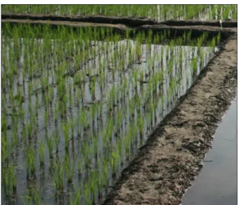
Uni Bonn (2010b), respectively. ... 21 Figure 3-1. Location of the study sites in China (modified from Gnyp et al. (2013). ... 25 Figure 3-2. Overview of the investigated field experiment from scan position six (Figure 3-3).

On the right side the scanner with the tripod mounted on the small trailer can be seen

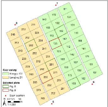
(taken: 04.07.11). ... 27 Figure 3-3. Experimental design and scan positions of the field experiment. Number in the plot

represents: rice variety (1 = Kongyu 131; 2 = Longjing 21); treatment (1 - 9 in Table 3-1);

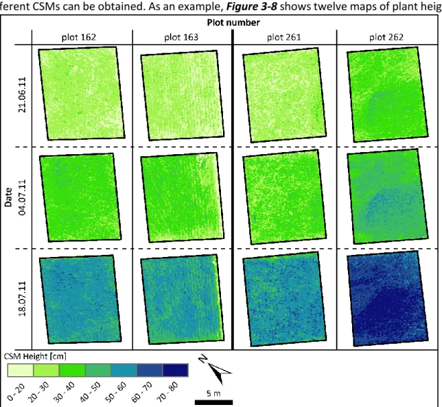
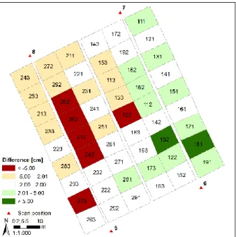
repetition (1 - 3). ... 28 Figure 3-4. Experimental design and scan positions of the farmer's field. ... 28 Figure 3-5. General overview of the workflow for the post-processing of the TLS data. ... 30 Figure 3-6. Corner of the field experiment, showing the least dense vegetation (taken: 21.06.11). .... 31 Figure 3-7. General concept of crop surface models (CSMs) (Bendig et al., 2013). ... 32 Figure 3-8. CSM-derived maps of plant height for four selected plots of the field experiment

(left: Kongyu 131; right: Longjing 21, marked in Figure 3-3). ... 33 Figure 3-9. Maps of plant growth for two selected plots of the field experiment, derived from the

difference between two consecutive CSMs (left: Kongyu 131; right: Longjing 21, marked in

Figure 3-3). ... 34 Figure 3-10. Difference between the averaged manually measured plant heights and the

CSM-derived mean plant heights for each plot for the first campaign of the field experiment. ... 35 Figure 3-11. Regression of the mean CSM-derived and manually measured plant heights for the

field experiment (n = 162) and the intensively investigated units on the farmer's field (n = 72). .... 36 Figure 3-12. Regression of the mean CSM-derived plant height and dry biomass for the field

experiment (n = 90) and the intensively investigated units on the farmer's field (n = 72). ... 37 Figure 3-13. Theoretical biomass simulated with regression model and the measured values for

the intensively investigated units on the farmer's field (each: n = 72). ... 38

(12)

Figure 4-1. Design of the field experiment and scan positions. Three-digit number in the plot represents rice variety (1 = Kongyu 131; 2 = Longjing 21); treatment (1 to 9); and repetition

(1 to 3). Modified from Tilly et al. (2014). ... 51

Figure 4-2. One management unit with very heterogeneous plant growth in village 36. ... 51

Figure 4-3. Scan positions and bamboo stick positions on the farmer’s fields. ... 53

Figure 4-4. Small, round reflectors were permanently attached to trees in village 36. ... 54

Figure 4-5. Crop surface model (CSM)-derived maps of plant height for two field experiment plots of both years, given with mean plant height per plot. ... 57

Figure 4-6. Regression of the mean CSM-derived and manually measured plant heights of the field experiment of both years (each n = 162). ... 58

Figure 4-7. Linear (left) and exponential (right) regression between mean CSM-derived plant height and dry biomass for the field experiment of both years (each n = 90); regression equations are given in Table 4-5. Biomass values for the exponential regression are natural log-transformed. ... 61

Figure 5-1. a) TLS system (marked with arrow) mounted on a cherry picker; b) highly reflective cylinders arranged on ranging pole. ... 73

Figure 5-2. CSM-derived maps of plant height for the whole maize field on the last campaign date (top) and for the buffer area around sample point 5 on each date (bottom). ... 75

Figure 5-3. CSM-derived maps of plant growth for the whole maize field (at the top between 3rd and 31st of July; at the bottom between the 31st of July and the 24h of September). ... 76

Figure 5-4. Regression of the mean CSM-derived plant height and the dry biomass (n = 48). ... 78

Figure 5-5. Regression of the mean CSM-derived and manually measured plant heights (n = 60). ... 78

Figure 6-1. Instrumental set-up: (A) terrestrial laser scanner Riegl LMS-Z420i; (B) tractor with hydraulic platform; (C) ranging pole with reflective cylinder. ... 87

Figure 6-2. Workflow for the calibration and validation of the biomass regression models and distinction of cases for each model. ... 91

Figure 6-3. Maps of four plots from the last six and five campaigns of 2013 and 2014, respectively. One plot of each N fertilizer level of the barley cultivar Trumpf is shown for each year (: Plot mean height). ... 92

Figure 6-4. Regression of the mean CSM-derived and manual measured plant heights (2012: n = 131; 2013: n = 196; 2014: n = 180). ... 93

Figure 6-5. Scatterplots of measured vs. estimated dry biomass for one validation data set for NDVI, RGBVI, REIP, and GnyLi (exponential model). Pre-anthesis: crosses and solid green line; whole observed period: circles and dashed black line; 1:1 line: light grey. ... 97

Figure 6-6. Scatterplots of measured vs. estimated fresh biomass for one validation data set for NDVI, RGBVI, REIP, and GnyLi (exponential model). Pre-anthesis: crosses and solid green line; whole observed period: circles and dashed black line; 1:1 line: light grey. ... 98

Figure 6-7. Scatterplot for one validation data set for the pre-anthesis (green) and for the whole observed period (black) of the bivariate BRM of PH (circles and solid regression line) and multivariate BRM of PH and GnyLi (crosses and dashed regression line) for dry biomass (top) and fresh biomass (bottom) (all exponential models); 1:1 line: light grey. ... 99

Figure 7-1. Platforms for TLS with the approximate sensor height: (A) Tripod (1.5 m); (B) Tractor- trailer system (3 m); (C) Tractor with hydraulic platform (4 m); (D) Cherry picker (8 m). ... 116

Figure 7-2. Influence of the sensor height and the resulting inclination angle on the incidence angle. This affects which plant parts are ascertainable, which in turn influences the calculated mean plant height. Single plants modified from Large (1954). ... 117

(13)

Figure 7-3. Influence of platform movements during the scans on the calculated maize plant heights. Scans were acquired from the basket of the cherry picker, placed close to the corners of the field. ... 119 Figure 7-4. Plant heights ascertainable from the TLS-derived point clouds and the manual

measurements. The measuring processes influence the calculated mean plant height. Single plants modified from Large (1954). ... 120 Figure 7-5. Averaged CSM-derived vs. manually measured plant heights of all campaigns on

paddy rice, maize, and barley (left) and of all except maize (right). ... 121 Figure 7-6. Mean trend of plant height and dry biomass of barley across the growing season with

trend curves as polynomial functions of the 3rd degree. ... 124 Figure 7-7. Dry biomass accumulation in crop parts. Modified from Fischer (1983). ... 125 Figure 7-8. Dry biomass map of the paddy rice units in village 36 for the 16.07.2012. Estimated

from the CSM-derived plant height with the BRM: Biomass = 12.37 ∙ plant height - 273.19

(Table 4-5). ... 126 Figure 7-9. Assimilation in ripening cereal. Green color marks active plant parts. Modified from

Munzert and Frahm (2005). ... 128 Figure 7-10. MLS systems for crop monitoring: (A) Phenomobile (Deery et al., 2014); (B) LiDAR

sensor, attached to a combined harvester (Lenaerts et al., 2012). ... 130 Figure 7-11. Low-altitude airborne platforms: (A) MikroCopter Okto XL with hyperspectral

snapshot camera (modified from Aasen et al., 2015); (B) Gyrocopter (Weber et al., 2015). ... 132

(14)

Tables

Table 2-1. Chronological selection of TLS systems with maximal measuring rate (Large and

Heritage, 2009; Riegl LMS GmbH, 2015a, 2013). ... 10

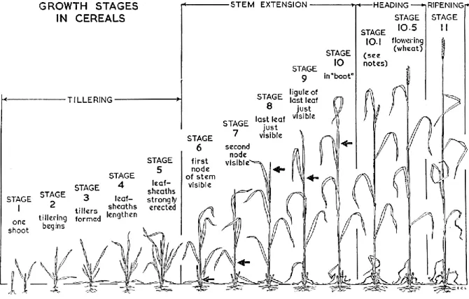
Table 2-2. Principal growth stages of the BBCH scale and criteria for their subdivision in developmental steps, modified from Meier (2001). ... 14

Table 2-3. Equations of the biomass regression models. ... 18

Table 3-1. Fertilizer application scheme for both study sites. ... 26

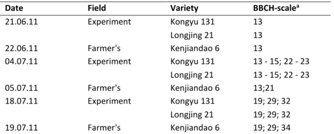
Table 3-2. Dates of the scan campaigns and corresponding phenological stages. ... 27

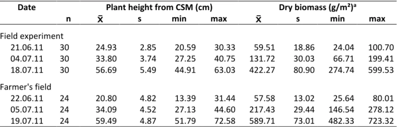
Table 3-3. Mean CSM-derived and manually measured plant heights for both fields... 35

Table 3-4. Mean CSM-derived plant heights and biomass values. ... 36

Table 3-5 Biomass values for the overall farmer's field. ... 38

Table 4-1. Dates of the terrestrial laser scanning (TLS) campaigns and corresponding phenological stages. ... 52

Table 4-2. Mean crop surface model (CSM)-derived and manually measured plant heights of the field experiment (n: number of samples; : mean value; SD: standard deviation; min: minimum; max: maximum). ... 58

Table 4-3. Mean CSM-derived plant heights and destructively measured biomass values of all sites (n: number of samples; : mean value; SD: standard deviation; min: minimum; max: maximum). ... 59

Table 4-4. Trial biomass regression models (BRMs) and validation of estimated against measured biomass (R²: coefficient of determination; d: index of agreement; RMSE: root mean square error). ... 60

Table 4-5. Biomass regression models (BRMs), derived from field experiment and validation of estimated against measured biomass for the farmer’s fields (R²: coefficient of determination; d: index of agreement; RMSE: root mean square error). ... 61

Table 5-1. CSM-derived and manually measured plant heights as well as destructively taken biomass, based on the averaged values for the buffer areas (each date n = 12). ... 77

Table 6-1. Dates of the terrestrial laser scanning (TLS) and spectrometer (S) campaigns listed as day after seeding (DAS). Averaged codes for the developmental steps are given for the dates of manual plant parameter measurements (BBCH). For some dates BBCH codes were not determined (N/A). ... 85

Table 6-2. Principal growth stages of the BBCH scale. ... 86

Table 6-3. Vegetation indices used in this study. ... 90

Table 6-4. Statistics for the plot-wise averaged CSM-derived plant heights and destructively taken biomass for the reduced data sets of 2013 and 2014 (n: number of samples; : mean value; min: minimum; max: maximum; SD: standard deviation). ... 94

Table 6-5. Statistics for the model calibration as mean values of the four subset combinations (R²: coefficient of determination; SEE: standard error of the estimate). ... 95

Table 6-6. Statistics for the model validation as mean values of the four subset combinations (R²: coefficient of determination; RMSE: root mean square error (g/m²); d: Willmott’s index of agreement). ... 96

Table 7-1. Advantages and disadvantages of the platforms used for field surveys. ... 119

Table 7-2. R² values for linear and exponential regression between CSM-derived plant height and dry biomass for the field experiments. ... 123

(15)

Abbreviations

ALS Airborne laser scanning

AOI Area of interest

BBCH Biologische Bundesanstalt (German Federal Biological Research Centre for Agriculture and Forestry), Bundessortenamt (German Federal Office of Plant Varieties), and Chemical industry

BRM Biomass regression model

CSM Crop surface model

d Willmott’s index of agreement

DAS Day after seeding

DEM Digital elevation model

DGPS Differential global positioning system

DSM Digital surface model

DTM Digital terrain model

FAO Food and Agriculture Organization of the United Nations

GNSS Global navigation satellite systems

ICP Iterative closest point

IDW Inverse distance weighting

IMU Inertial measurement unit

LAI Leaf area index

LiDAR Light detection and ranging

MLS Mobile laser scanning

N Nitrogen

NDVI Normalized difference vegetation index

NIR Near-infrared domain

NNI Nitrogen nutrition index

NRI Normalized reflectance index

PA Precision agriculture

PH Plant height

PLS Personal laser scanning

R² Coefficient of determination

RDVI Renormalized difference vegetation index

REIP Red edge inflection point

RGBVI Red green blue vegetation index

RMSE Root mean square error

S Spectrometer

SAR Synthetic aperture radar

SEE Standard error of the estimate

SWIR Shortwave infrared domain

TLS Terrestrial laser scanning

UAV Unmanned aerial vehicle

VI Vegetation index

VIS Visible domain

VISNIR Visible and near-infrared domain

(16)

1 Introduction 1.1 Preface

The rapidly growing world population and the related demand for food security causes challenges for agri-food researchers (Marsden and Morley, 2014). According to the figures of the Food and Agriculture Organization of the United Nations (FAO) the total cereal production increased from ~2.0 to ~2.8 billion tons over the last 20 years (FAO, 2014). In the same period, the worldwide harvested area for cereals stayed almost constant at

~700 million hectares,

which underlines the pressure on the efficiency of land use. Moreover, the FAO indicates that within this 20 years the world population rose from ~5.5 billion to ~7.1 billion people, with a supposed rise up to ~8.6 billion within the next 20 years. By the middle of this century already

~10 billion world citizens are expected. This growing population demands a secure food

supply, which in turn increases the pressure on the conventional agricultural sector and requires an improvement of management methods (Liaghat and Balasundram, 2010).

Fortunately, an increasing recognition of the interaction between production and consumption and between food security and sustainability is observable in large sections of the population (Marsden and Morley, 2014). Since the 1990’s technical management methods and practices which aim at improving the food production emerged and can be summarized under the term precision agriculture (Mulla, 2012). One of the first definitions for precision agriculture came from the US House of Representatives and stated it as “an integrated information- and production-based farming system that is designed to increase long-term, site specific and whole farm production efficiencies, productivity, and profitability while minimizing unintended impacts on wildlife and the environment” (US House of Representatives, 1997). Considering the topic of this thesis, this definition should be narrowed to the term site-specific crop management to differentiate from animal industries or forestry (Whelan and Taylor, 2013). Related approaches address the improvement of farming practices to better suit soil and crop requirements. However, both terms precision agriculture and site- specific crop management are often used synonymously.

Based on these definitions two main aspects in this research field can be derived (Whelan and Taylor, 2013). First, from an economic point of view, improving the productivity of crops, which means the harvested yield, is obviously most important. Second, from an ecological point of view, exhausting or polluting soil, groundwater, and the entire environment through intensive field management needs to be minimized or, even better, avoided.

Generally, a number of natural and human-induced processes are relevant for site-specific crop management and moreover they can show spatial and temporal variations (Oliver, 2013).

These changes across time involve differences between the growing seasons, but also within

one season. Beside quite stable factors, such as the physical landscape, climate, and biological

lifecycle of crops, the efficiency of an agricultural production depends on varying weather

conditions and field management practices for example (Atzberger, 2013). Hence, the

required frequency of measurements to observe temporal variations depends strongly on the

concrete issue. In contrast to these factors which are generally quite uniform across regions,

spatial variabilities can be detected between adjacent fields and moreover within one field.

(17)

Possible sources are fertilizer residues in the ground, varying water availability, or generally small-scale heterogeneities of soil properties. The importance of detecting in-field variations for site-specific crop management can be demonstrated by the example of Whelan and Taylor (2013), shown in

Figure 1-1. The average yield and amount of variation are equal in

both fields, but the patterns differ. It is obvious that for an acquisition of patterns such as in the right field (B), measuring systems with a high in-field resolution are required.

Today, sensor-based approaches are already findable for some applications assignable to precision agriculture. Such technologies can support plant protection and site-specific seeding (Auernhammer, 2001) or the detection of foliar diseases (Lee et al., 2010). With the aim of enhancing the yield, precision agriculture is frequently associated with site-specific fertilization (Auernhammer, 2001). Xu et al. (2014), for example, showed that appropriate fertilizer recommendations can increase the grain yield and moreover reduce the nutrient loss and environmental pollution. In this context, biomass estimations are of major interest, since studies show that crop yield is correlated to biomass (Boukerrou and Rasmusson, 1990;

Fischer, 1993). This correlation can be quantified by the harvest index, expressing the yield versus total dry biomass (Price and Munns, 2010). Hence, accurately determining biomass can help to forecast yield.

Beyond the yield-correlated amount of biomass at the end of the growing season, the in-season status of the plants is more important. One reason therefore is that adequate conditions during early growing stages could preserve the yield against challenges of later stages, caused by drought stress for example (Bidinger et al., 1977). An essential prerequisite for optimizing plant conditions through adequate field management is to acquire the current state of the crop and monitor changes. A benchmark for quantifying the plant status in-season is the nitrogen nutrition index (NNI), showing the ratio between actual and critical nitrogen (N) content (Lemaire et al., 2008). Since this critical value corresponds to the actual crop biomass, a precise determining of biomass is desirable.

A major difficulty for all biomass-related indices is that a non-destructive determination of biomass is not possible. This is why several approaches focus on its estimations based on other parameters. Remote sensing methods were therefore increasingly applied over the last several decades (Mulla, 2012). Casanova et al. (1998), for example, measured the reflectance on rice plants across the growing season with a hand-held radiometer and attained very good

Figure 1-1. Patterns of spatial variability. The average yield (2.5 t/ha) and the amount of variation (50% = 1 t/ha; 50% = 4 t/ha) are the same in (A) and (B), but the patterns differ (Whelan and Taylor, 2013).

(A) (B)

(18)

results for the estimation of biomass at field scale; 97 % of the variance in biomass could be explained by their model. On a far greater observation scale, satellite-based remote sensing enables to capture entire regions in a short time. As shown by Claverie et al. (2012), remote sensing data with a high spatial and temporal resolution, in this case Formosat-2 images, can be used to estimate biomass. Through the daily revisit time of the satellite, the authors obtained a comprehensive data set and well estimated biomass, with a relative error of 28 %.

However, a main issue for all approaches based on optical satellites is the dependence on cloud-free conditions. In their first observation year Claverie et al. (2012) obtained only 27 almost cloud-free images from a total number of 51. Active satellite-based remote sensing systems, such as synthetic aperture radar (SAR) sensors, are used to overcome this problem (Koppe et al., 2012; Zhang et al., 2014). Nevertheless, referring to the variability of processes which influence site-specific crop management, the temporal resolution reachable with a satellite-based system always depends on the satellite revisit time, which limits the flexibility of the approach. Regarding the spatial resolution, only recently systems have been developed which allow surveys with a high in-field resolution. One example is WorldView-3 with a pixel size of ~0.3 m (DigitalGlobe, 2014). Between these approaches, which regarded very different observation levels, numerous studies on crop monitoring with different remote sensing sensors are findable across almost all scales.

It can be summarized, that in the field of precision agriculture or rather site-specific crop management, a growing demand arises for approaches on monitoring plant parameters with a spatial in-field resolution. Parameters usable for reliable biomass estimations are thereby of major importance. In general, the required temporal and spatial resolution is very case-specific, but timely flexible systems which allow a high spatial resolution are desirable, since the influencing environmental factors are variable in time and space (Atzberger, 2013).

Moreover, they should be as robust as possible against poor weather conditions and ideally almost independent from external factors, such as solar radiation.

1.2 Research issue and study aim

The request for the reliable determination of biomass motivates the overall aim of this study: developing a robust method for the non-destructive estimation of crop biomass at field scale. Looking at the literature, biomass-related parameters, such as plant height, leaf area index (LAI), or crop density are assumed to be suitable estimators. Having regard to ground- or vehicle-based measurements, plant parameters like crop density, LAI, or directly biomass are widely estimated with vegetation indices (VIs) from spectral data (Casanova et al., 1998;

Clevers et al., 2008; Gnyp et al., 2014b; Montes et al., 2011; Thenkabail et al., 2000). Therein,

the reflectance is often measured with passive sensors, having disadvantages like the

dependency on solar radiation and the influence through atmospheric conditions. Since these

factors are variable in space and time, a site-specific spectral calibration is required

(Adamchuk et al., 2004), which has to be frequently repeated during the measurements

(Psomas et al., 2011). This makes surveys quite laborious.

(19)

In contrast, an active system like terrestrial laser scanning (TLS) operates with a self-generated signal, making the measurements independent from an external light source (Briese, 2010). In addition, the system is flexible for the application in the field as the scanner can be established on a tripod or small vehicle. The result of a TLS survey is a very dense 3D point cloud, representing the spatial distribution of reflection points in the area of interest (AOI), but measured with one wavelength. This makes a derivation of VIs impossible but enables to easily capture the entire field. Consequently, the question is how to derive plant parameter information from the TLS data?

In this work, the 3D point cloud from each TLS campaign is interpolated to a crop surface model (CSM). CSMs were introduced by Hoffmeister et al. (2010) to represent the entire crop canopy with a very high spatial resolution at a specific date. At each site multi-temporal CSMs are established based on several campaigns. By subtracting a digital terrain model (DTM) of the bare ground from each CSM, plant heights are calculated pixel-wise and stored as raster data sets. These measurements of plant height are then used for estimating biomass. First promising results for the estimation of aboveground biomass were already attained in a feasibility study for sugar beet by Hoffmeister (2014), but regarding world nutrition sugar beet plays a minor role. The most important group of crops are cereals due to their high proportion of carbohydrates (FAO, 1994). In view of the worldwide harvested area the five most important cereals are wheat, maize, paddy rice, barley, and rye, which cover already more than 85 % of the total area. Cereals might be further grouped in three categories by their general appearance and cultivation methods. Except for maize, which is clearly distinguishable through the larger plant height and paddy rice, which is grown on flooded fields, the remaining wheat, barley, and rye share main characteristics like plant heights of ~1 m and the cultivation on regular arable land.

A comprehensive investigation of this novel approach in terms of its usability for monitoring cereals at field scale is targeted in this study. Hence, the main aims are (I) to demonstrate the usability of TLS-derived point clouds for establishing CSMs, (II) to obtain plant height, and (III) to estimate cereal biomass from these plant height data. In four case studies biomass regression models (BRMs) are therefore empirically developed with three cereals as examples, namely paddy rice, maize, and barley. According to the above stated subdivision, all three categories of cereals are covered by these examples. In addition to the bivariate BRMs, a comparison with estimations based on VIs is performed and first steps towards a fusion of both parameters are carried out by establishing multivariate BRMs. The working process can be divided into the following steps:

I. Execution of field surveys at three sites with different platforms over four years.

II. Construction of CSMs from each TLS-derived point clouds.

III. Calculation of plant height.

IV. Estimation of biomass based on plant height.

V. Comparison of plant height and VIs as individual estimators and fused in multivariate BRMs for the barley case study.

VI. Validation of plant height and estimated biomass against comparative data.

(20)

Generally, any remote sensing approach can be evaluated by its reachable spatial and temporal resolution (Campbell and Wynne, 2011). Thereby is the detection of spatial patterns limited by the size of the areas which can be separately recorded by the sensor. The repeatability in time strongly depends on the flexibility of the platform. According to these criteria the presented ground-based TLS approach shows promising potential for the acquisition of plant height at field scale. Consequently, the same high spatial resolution can be assumed for spatially resolved biomass estimations across the entire field. The major innovative aspects are in particular the possibility to capture entire fields, the very high spatial resolution, and the flexible usage. Moreover, the survey dates can be quite easily adapted to capture particular steps of the plant development or measurements can be postponed due to poor weather.

1.3 Outline

This chapter 1 should have given a first impression of how important crop monitoring is, in particular the acquisition of biomass-related parameters for site-specific crop management.

Within the framework of this study, a comprehensive data set was achieved, allowing to evaluate the potential of TLS-derived 3D data of plant height for estimating biomass at field scale. In the following chapter 2 fundamental basics therefore are given, including a summary about remote sensing, with particular attention on applications in agriculture and a general introduction into TLS. After that, the regarded cereals are briefly portrayed and the general crop development across the growing season is addressed. Then, existing approaches for crop monitoring are presented and the methodology requisite for the case studies is introduced.

This involves the construction of CSMs and the development of BRMs. In this context, the attainable scales and dimensions are regarded. Finally, the three case study sites are placed in a geographical context.

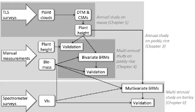
The chapters 3 to 6 contain the research papers, presenting the results of the case studies.

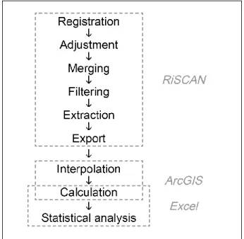
They are sorted along the overall workflow (Figure 1-2). Although, the major steps like the post-processing of the point clouds, the calculation of plant height, and the estimation of biomass are addressed in all papers, they are broadly assigned to the workflow according to their main focuses. First of all, the general concept of obtaining plant height from multi-temporal TLS-derived CSMs is examined in Tilly et al. (2014a; chapter 3) based on surveys on two paddy rice fields of one growing season. Moreover, the potential of CSM-derived plant height for estimating biomass is investigated. Then, in conjunction with these data sets, the measurements of two paddy rice fields from the subsequent growing season are analyzed in Tilly et al. (2015b; chapter 4). The main focus of this study lies on the spatial and temporal transferability of the BRMs. Concerning the data acquisition, the results of measurements on a larger field are shown for a maize field in Tilly et al. (2014b; chapter 5).

Furthermore, the applicability of a cherry picker as platform is investigated based on several

campaigns in one growing season. In Tilly et al. (2015a; chapter 6) the performances of plant

height and VIs as individual estimators are compared and first attempts of improving the BRMs

through fusing both parameters are carried out. A barley field experiment was therefore

monitored with TLS and with a field spectrometer over three growing seasons.

(21)

Based on the results of these case studies chapter 7 gives an overall discussion. In this, firstly some issues related to the field measurements are regarded. Then the reliability and utility of the CSM-derived 3D data of plant height is evaluated and the validity of the biomass estimations is assessed. This also includes an evaluation of the fusion with spectral data.

Afterwards, future prospects for laser scanning approaches in agriculture are outlined. Finally, Chapter 8 gives a concluding assessment of the applied methods and achieved results.

Figure 1-2. Overall workflow and allocation of research papers in the chapters 3 to 6 according to their main focuses.

(22)

2 Basics

2.1 Remote sensing

One of the earliest approaches commonly assigned to remote sensing is the use of balloons for aerial photography in the late 19

^th

century (Lillesand et al., 2004). Enabled through the development of airplanes, the interpretation of aerial photos increased in importance during the world wars (Jensen, 2007). In the late 1950s civilian applications of aerial photography arose as a source of cartographic information (Campbell and Wynne, 2011). From these approaches, the common aspect in definitions of remote sensing can be concluded:

sensor-based data acquisition to derive information about an object with a certain distance between sensor and object (Lillesand et al., 2004). Since no clear definition exists how great this distance is, a variety of sensors and platforms, from ground-based over low- and high-altitude airborne to spaceborne systems are currently included under the rubric of remote sensing. The former ones are sometimes referred to as proximal (remote) sensing.

Moreover, remote sensing might not be regarded as an own science, rather it is a tool or technology which is applied in a multitude of scientific disciplines (Löffler, 1985). In this respect - contemporaneously with the development of new sensors from a technical perspective - the application of remote sensing has reached more and more fields of human activity. Only looking at remote sensing of the natural environment, applications range already from the acquisition of data regarding vegetation and water to the assessment of soils, minerals, or geomorphological structures (Jensen, 2007). Extending the application fields to urban areas, further issues are, for example, the detection of city structures, like roads and buildings, detailed monitoring of production facilities, or human-induced changes of the natural environment, such as forest or agricultural land. With regard to the extent of this thesis, the focus of this chapter is narrowed to remote sensing in agricultural applications with different sensors and a more detailed introduction into TLS.

2.1.1 Application in agriculture

Remote sensing methods are widely used in agriculture, as they allow non-contact surveys and thus prevent disturbing the plants by the taking of measurements (Liaghat and Balasundram, 2010). Applied sensors and platforms range across almost all scales, from hand-held and tractor-based sensors to air- and spaceborne systems in micro-level to regional and global surveys, respectively (Allan, 1990). As for any application of remote sensing, major factors for choosing a system are the targeted spatial and temporal resolution. Mulla (2012) prognosticates that, compared to current approaches, future site-specific crop management will claim for greater spatial and temporal resolutions. Atzberger (2013) summarized the current research focuses of such approaches to five main topics: (I) crop yield and biomass, (II) crop nutrient and water stress, (III) infestations of weeds, (IV) insects and plant diseases, and (V) soil properties.

According to this subdivision, the presented study belongs to the first topic and hence the

following remarks are limited to applications dealing with crop biomass. Figure 2-1 lists several

remote sensing sensors and platforms, usable for biomass estimations. The selection is based

on recent exemplary studies of the last five years and cannot claim to completeness, rather it

(23)

should give a general view across methods at different observation scales. It has to be noted that an acquisition at an entire global scale is not very useful for agricultural applications.

This selection of studies demonstrates the general interest in the use of remote sensing methods for estimating biomass. Thereby advantages and disadvantages can be assumed for each system, considering factors like the spatial resolution, the possible temporal frequency of measurements, or the dependency on external sources. In this study, TLS was chosen as

Figure 2-1. Selection of remote sensing methods for the estimation of crop biomass across scales.

Content of the studies is summarized to sensor and regarded crop or grassland.

(24)

system which allows measurements at field scale in a high spatial resolution. In addition, the ground-based active sensor is fairly flexible and independently usable.

2.1.2 Terrestrial laser scanning

Out of the variety of remote sensing sensors TLS is quite a young discipline. It is assignable to the proximal sensing methods with a short sensor range, compared to satellite-based systems for example. However, in the beginning laser-based measurements were applied with greater distances between sensor and object (Jensen, 2007). The origin of laser-based distance measurements can be dated back to the development of the first optical laser in 1960. Since the 1970s light detection and ranging (LiDAR) systems based on aircrafts, also known as airborne laser scanning (ALS), were used for elevation mapping (Lillesand et al., 2004). In these early stages such measurements were primarily used in traditional engineering surveying, but caused by technical refinements and the development of weather-resistant systems during the late 20

^th

century, laser scanning aroused the interest of environmental scientists (Large and Heritage, 2009). In several cases the application of a plane was however not flexible enough or too expensive and the spatial resolution of ALS was not sufficient. The resulting demand for ground-based systems led to the evolution of TLS.

Only in the late 1990s the first TLS systems have been introduced, but the development of new sensors rapidly increased and their usage is now extended over a wide range of research areas (Large and Heritage, 2009). Applications of TLS range across various fields, such as geomorphology (Schaefer and Inkpen, 2010), geology (Buckley et al., 2008), forestry studies (van Leeuwen et al., 2011), archeology (Lambers et al., 2007), or urban mapping (Kukko et al., 2012). With the main advantage of easily capturing data in a high rate and density, TLS offers opportunities for non-experts, outside traditional surveying disciplines, to acquire 3D spatial information. Nevertheless, a basic understanding of the measuring principle is necessary. This can be exemplified by two simpler versions of laser-based measuring devices, namely laser ranging and laser profiling systems.

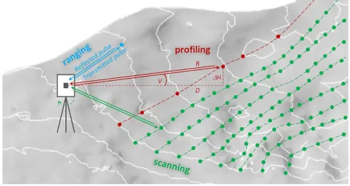
The basic principle of so called time-of-flight measurements can be explained with the laser ranger (Petrie and Toth, 2008). Emitted by the ranger, the laser radiation is used to accurately measure the travel time, or time-of-flight, between transmitting a signal and its return to the receiver after reflection on any point of an object, also referred to as reflection point (ranging in Figure 2-2). From this time-of-flight, the slant distance or range (R) between the ranger and the reflection point is calculated as half of the entire path, with the speed of light is known to be ~0.3 m/ns:

𝑅 =(𝑠𝑝𝑒𝑒𝑑 𝑜𝑓 𝑙𝑖𝑔ℎ𝑡 ∙ 𝑡𝑖𝑚𝑒 𝑜𝑓 𝑓𝑙𝑖𝑔ℎ𝑡) 2

In environmental science, rather than locating individual reflection points, capturing 2D profiles is desired for detecting terrain features. Similar as ranging systems, laser profiling devices measure the ranges (R) of several reflection points in equidistant steps along a line, but in addition the vertical angles (V) between R and the horizontal are observed (profiling in

Figure 2-2). The profile is then determined through calculating each horizontal distance (D)

and difference in height (H) between the sensor and the reflection points:

𝐷 = 𝑅 cos 𝑉 ∆𝐻 = 𝑅 sin 𝑉

(25)

Through adding a scanning mechanism to the system, such as a rotating mirror or a prism, a laser scanner is attained, which can measure the vertical dimension of a profile along a topographic features in a high detail (Petrie and Toth, 2008). Due to the static position of the terrestrial laser scanner, an additional motion is necessary to attain a horizontal resolution. Usually, a movable component, containing the scanning mechanism is rotated by an engine around the vertical axis, which allows to measure a series of parallel profiles (scanning in Figure 2-2). The result of one measurement is then a cluster of reflection points, known as point cloud, containing the x, y, and z coordinates of each point.

In the short history of TLS, the measuring rate of reflection points has rapidly increased with the development of new systems. While the first launched sensor Leica Cyrax 2400 was capable of measuring only 100 point/sec, the sensors used in the case studies of this thesis measure 100 to 1,000 times more points/sec.

Table 2-1 gives an overview about selected

systems, whereby the selection is limited to time-of-flight scanners, since only such systems were used in this study. Beyond that, phase scanning systems should be mentioned as available alternatives, which achieve higher measuring rates and a better accuracy, but can only measure in shorter ranges (Beraldin et al., 2010). Their measuring principle differs slightly from time-of-flight scanners. Phase scanners emit the laser beam at alternating frequencies and measure the phase difference between the emitted and reflected signal.

Table 2-1. Chronological selection of TLS systems with maximal measuring rate (Large and Heritage, 2009; Riegl LMS GmbH, 2015a, 2013).

Launch year Sensor Maximal measuring rate

1998 Leica Cyrax 2400 100 points/sec

2001 Leica Cyrax 2500 1,000 points/sec

2007 Riegl LMS-Z420i ^a 11,000 points/sec

2007 Leica ScanStation 2 50,000 points/sec

2010 Riegl VZ-1000 ^a 122,000 points/sec

2014 Riegl VZ-2000 400,000 points/sec

a Sensors used for the case studies.

Figure 2-2. Principle of time-of-flight measurements with laser ranging, profiling, and scanning systems.

(26)

2.2 Crops

In the framework of this study, time-of-flight scanners are used to monitor crop height across the growing season. According to the definition of the FAO, crops are agricultural products, coming directly from the field without any real processing, except cleaning (FAO, 2011). They might be further subdivided into cereals, pulses, roots and tubers, sugar crops, oil-bearing crops, fiber crops, vegetables, tobacco, fodder crops, fruits and berries, nuts, spices and aromatic herbs, and other crops (coffee, cacao, tea, and hops). In addition, it can be distinguished between temporary crops, being sown and harvested during the same growing season (sometimes more than once per year), and permanent crops, which have not to be replanted after each annual harvest.

The most important group of crops are cereals, as they contribute the most to world nutrition. In general, cereals are annual plants of the gramineous family, characterized by carbohydrate as main nutrient element (FAO, 1994). According to the statistics of the FAO, the five largest cereals alone (wheat, maize, paddy rice, barley, and rye) make up more than 85 % of the total harvested area for cereals (Figure 2-3). Based on their general appearance and growing characteristics three categories of cereals might be classified. Most cereals like wheat, barley, and rye reach plant heights of

~1 m and are grown on regular arable land.

Exceptions from this are maize due to the larger plant height and paddy rice due to its cultivation on flooded fields. All herein regarded examples (paddy rice, maize, and barley) are cereals and corresponding to this subdivision, they cover all subcategories and are thus regarded as suitable representatives for cereals. However, the broader term crop is preferred in the further course of the work as the presented concept of monitoring is transferable to other groups. Brief characterizations of paddy rice, maize, and barley are given in the following sections, listed in the order of their appearance in the chapters 3 to 6. Afterwards some general characteristics of crop growth and development are given as a basis for the concept of crop monitoring.

Wheat 31%

Maize 25%

Paddy rice 23%

Barley 7%

Rye

1% Other

13%

Worldwide harvested area for cereal Mean 2011 - 2013

Absolute values (ha)

Wheat 220,000,000

Maize 180,000,000 Paddy rice 160,000,000 Barley 50,000,000

Rye 5,000,000

Other 95,000,000

Total 710,000,000

Figure 2-3. Worldwide harvested area for the five main cereals.

Values according to FAO (2014).

(27)

2.2.1 Paddy rice

Cultivated rice (Oriyza) is the staple food for two thirds of the world population and the leading food crop in developing countries (Juliano, 2004). It is a cereal grain grass (family

Poaceae) and although it is an annual species, it may grow more than once per year under

reasonable environmental conditions. This quality of growth is influenced by factors like temperature, day length, nutrition, planting density, and humidity (Nemoto et al., 1995). Even though rice was originally a plant of wetlands, some species are cultivated on dry land or in water. It is common practice to flood the paddy rice fields for irrigation and simplifying weed control. The term paddy is the anglicized form of the Malayan word padi, meaning ‘of rice straw’ (Arendt and Zannini, 2013). Today, the term paddy rice is used for both the water-covered fields and the harvested product.

Historically, the most ancient archaeological findings of rice cultivation were found in the Yangzi delta in China, dating back to 5,000 BC (Arendt and Zannini, 2013). Although with almost 30 %, meaning about 200 Mio tons per year, China still accounts for the largest part of the world rice production, the cultivation of rice is nowadays widely distributed around the world. It is grown in more than 100 countries between 53° N and 40° S and from sea level to altitudes of up to 3,000 m, covering in total about one quarter of the worldwide harvested area for cereals (Figure 2-3). Assumable about

~100,000 rice varieties exist, of which only

a small number is cultivated (Juliano, 2004).

The appearance of the rice plants is marked by round and hollow stems with flat sessile leaf blades and a terminal panicle (Arendt and Zannini, 2013). Several stems are grouped to hills with fibrous roots at the bottom. Each stem is enveloped by leaf sheath, which continuously merge into the leaf blade. The height of the majority of the rice varieties ranges between 1 and 2 m at their final growth.

2.2.2 Maize

Cultivated maize (Zea mays L.), also known as corn, is along with wheat and rice one of the most extensively cultivated cereals (Arendt and Zannini, 2013). It is an important source for a wide range of applications, such as human diet, feeding animals, or production of fuel and fibers. For a long time different theories on the origin of maize existed (Lee, 2004). The widely shared assumption today is that it was domesticated at least 6,700 BC in the highlands of Mexico. Nowadays, cultivated areas are spread worldwide, horizontally between 50° N and 40° S and vertically from the Caribbean islands to 3,400 m above sea level in the Andean mountains. About one quarter of the worldwide harvested area for cereals in more than 160 countries is cultivated with maize (Figure 2-3).

Like paddy rice, maize is a cereal grain grass of the family Poaceae, sharing characteristics such as conspicuous nodes in the stem and a single leaf at each node, with leaves alternately arranged (Lee, 2004). On the contrary, final plant heights are much larger; typically maize plants reach heights of 2.0 - 3.5 m. Plant height and yield are obviously influenced by environmental factors, irrigation, and fertilization.

2.2.3 Barley