Waves in heterogeneous media: long time behavior and dispersive models

Waves in heterogeneous media:

Long time behavior and dispersive models

Dissertation

zur Erlangung des Grades eines Doktors der Naturwissenschaften

Der Fakult¨at f¨ur Mathematik der Technischen Universit¨at Dortmund

im Juni 2011 vorgelegt von

Agnes Lamacz

Tag der m¨ undlichen Pr¨ ufung: 06.09.2011 Pr¨ ufungskommission:

Vorsitzender: Prof. Dr. H.Blum Erster Gutachter: Prof. Dr. B. Schweizer Zweiter Gutachter: Prof. Dr. M. R¨oger Weiterer Pr¨ufer: Prof. Dr. K.F. Siburg Wiss. Mitarbeiter: Dr. A. R¨atz

Contents

I Introduction 4

1 Introduction to homogenization theory 4

1.1 Elliptic homogenization problem . . . . 5

1.2 Elliptic homogenization result . . . . 6

1.3 Homogenization of the wave equation . . . . 10

2 Long time homogenization of waves and main results 13 2.1 Main results in the one-dimensional case . . . . 13

2.2 Main results in an abstract framework and the multi-dimensional case . . . . 17

II The one-dimensional case 21

3.2 Equation for v_ε in the moving frame . . . . 23

3.3 Proof of Theorem 2.7 . . . . 24

4 The original homogenization problem and the weakly dispersive equation 28 4.1 The weakly dispersive problem . . . . 28

4.2 The adaption operator . . . . 29

4.3 Proof of Theorem 2.5 . . . . 32

5 Construction ofA_ε and algebraical properties 35 5.1 Construction of the auxiliary problems . . . . 35

5.2 Algebraical simplifications . . . . 37

5.3 Effect of the wave operator on A_ε(vε) . . . . 39

III Abstract framework and the multi-dimensional case 42

6.2 Other energy densities . . . . 46

6.3 Fine properties of solutions forN = 1 . . . . 47

7 Effective speeds and Riemannian distance 49 7.1 Domains of dependence . . . . 49

7.2 Riemannian distance and Hamilton-Jacobi equations . . . . 50

7.3 Geometric effective cone of dependence and effective speeds . . . . 54

7.4 Geometric effective speed in one space dimension . . . . 56

7.5 Analysis of ¯cby means of waves in stratified media . . . . 58 8 Estimate for the N-dimensional energy measure 60 A Energy estimate for the time-scaled wave equation 62

Part I

Introduction

1 Introduction to homogenization theory

The development of the mathematical theory ofhomogenization is strongly related to the requirement to describe the behavior of composite materials.

Composite materials consist of two or more individual constituents. They are finely mixed and look almost homogeneous from a macroscopic point of view. On a much smaller microscopic scale, the ingredients are separated. In other words, the heterogeneities of a composite determine a specific length scale, the microscopic scale, which is very small compared to the global dimension of the material, which in turn characterizes the macroscopic scale.

According to the fact that composite materials in general exhibit better properties than their ingredients, they are widely used in industry, see for instance pavement in roadways or superconducting multi filamentary composites in optical fibers. However, especially from the numerical point of view the small heterogeneities are very hard to treat. They produce a wide range of fluctuations and oscillations, which considerably affect the global behavior of the material.

The aim of the homogenization theory is to describe the global properties of a given composite medium. More precisely, the aim is to replace the highly oscillating characteristics of the composite in question by constant, usually referred to aseffective quantities, which in turn correspond to a homogeneous material, called the effective material.

In what follows we will always suppose that the heterogeneities of the composite in question are evenly distributed, which is a perfectly appropriate assumption for a wide range of applications. One natural way to express this assumption in a mathe- matical model is to consider periodically inhomogeneous media, where the periodicity length (and thus the characteristic length of the micro-scale) is represented by a small parameter ε >0, see Fig 1.

Figure 1: An ε-periodic composite material occupying a domain Ω. The material consists of two ingredients.

The notion ofmathematical periodic homogenizationindicates the process of taking ε→0 and the study of solutions u_ε of corresponding ε-problems in this limit.

In the last 40 years several books have been devoted to the periodic and non- periodic homogenization theory, see for instance [5, 10, 18] for a general overview. In this introductory section we will present the most fundamental classical results and methods in this field.

1.1 Elliptic homogenization problem

In this subsection we introduce the most elementary periodic homogenization problem of investigating solutionsuε to the elliptic problem

−∇ · Ax

ε

∇u_ε(x)

=f(x). (1.1)

It is made more precise in Definition 1.2 below.

In fact, Eq.(1.1) is a widely studied model case. On the one hand it models thermal, electrical and elastic properties of composites, which are encoded in the ε-periodic matrixA _ε^·

. It is thus relevant for many applications. On the other hand, already in this relatively simple setting the main mathematical difficulties in the homogenization process, ε→0, become obvious.

Let us first of all introduce a class of admissible matrices to guarantee the well- posedness of problem (1.1).

Definition 1.1 (Class of admissible matrices). Let N ∈ N and let 0 < α < β. We denote by M(α, β) the set of all matrices A∈R^N×N such that for every λ∈R^N there holds

hAλ, λi ≥α|λ|²,

|Aλ| ≤β|λ|,

where h·,·i denotes the scalar product in R^N and |λ| is the length of λ.

We are now in the position to introduce the classical elliptic homogenization prob- lem with Dirichlet boundary conditions.

Definition 1.2 (Elliptic homogenization problem). Let 0 < α < β and let Ω ⊂ R^N be open and bounded. Let A(·) = (a_ij(·))1≤i,j≤N ∈ C^∞(Ω,R^N×N) be such that A(x) ∈ M(α, β) for every x∈Ω. Moreover, let A(·) be (0,1)^N-periodic, A(x+e_i) =A(x) for every i= 1, ..., N, where e_i denotes the i-th unit vector in R^N. We call u_ε ∈H¹(Ω) a solution to the elliptic homogenization problem if

−∇ · Ax

ε

∇u_ε

=f in Ω,

u_ε = 0 on ∂Ω

(1.2) in the weak sense for f given in H⁻¹(Ω), the dual space of H₀¹(Ω).

We remark that due to the (0,1)^N-periodicity of the matrix A(·), the coefficient A _ε^·

is (0, ε)^N-periodic and thus highly oscillating.

By the Lax-Milgram theorem there exists a unique solution uε ∈ H₀¹(Ω) to the elliptic problem of Definition 1.2. Moreover, the following uniform (in ε) estimate holds

ku_εk_H¹

0(Ω)≤ 1

αkfk_H⁻¹_(Ω). (1.3)

Consequently, there exists some u ∈ H₀¹(Ω) such that, up to a subsequence, u_ε con- verges weakly to u as ε goes to zero, u_ε* u inH₀¹(Ω).

At this point, two natural questions arise.

1. Isuuniquely determined in the sense that every subsequence of u_ε converges to the same limit function u?

2. Which effective problem is solved by u?

Already in the 1970s both questions have been answered, see for instance Sanchez- Palencia [26, 27] or Bensoussan, Lions and Papanicolaou [5]. The result, see Theorem 1.3 in the next subsection, is now standard.

1.2 Elliptic homogenization result

In this subsection we state the classical homogenization result for elliptic problems and briefly present the three classical homogenization methods in the periodic framework:

1. Formal asymptotic expansions 2. Oscillating test functions 3. Two-scale convergence

While the first method is just a formal approach, the second and the third one are rigorous and provide proofs of the classical homogenization result stated below.

Theorem 1.3 (Classical homogenization result for elliptic problems). Let uε be the solution to the elliptic homogenization problem of Definition 1.2. Then

u_ε * u₀ in H₀¹(Ω), Ax

ε

∇u_ε * A^∗∇u₀ in (L²(Ω))^N,

where the limit function u₀ ∈ H₀¹(Ω) is the unique solution to the effective constant coefficient problem

−∇ ·(A^∗∇u₀) = f in Ω,

u₀ = 0 on ∂Ω. (1.4)

The matrix A^∗ = (a^∗_ij)1≤i,j≤N is given through a^∗_ij =

Z

(0,1)^N

a_ij(x) dx− Z

(0,1)^N N

X

k=1

a_ik(x)∂χˆ_j

∂y_k(x) dx, (1.5) where the functionsχˆ_j(·), often referred to as correctors, are(0,1)^N-periodic and solve specific auxiliary cell problems. They are defined in (1.8).

Theorem 1.3 suggests that the whole sequence (question 1 in the previous subsec- tion) converges to the function u₀. The limit function u₀ solves a constant coefficient problem of exactly the same type as the original problem (question 2).

Let us draw the readers attention to a peculiarity of the homogenization process.

Contrary to what one would expect at first sight, the effective matrixA^∗is not just the mean value of the oscillating coefficient A(·). Formula (1.5) suggests that in fact the mean value ofA(·) has to be corrected by additional terms which include the gradients of specific auxiliary functions.

In what follows we will not perform the proof of Theorem 1.3 in detail, which can for instance be found in [10]. Instead we will briefly present the three classical methods mentioned above. By means of asymptotic expansions we will show how formula (1.5) can be formally justified. By means of oscillating test functions and two-scale convergence we will sketch two quite different ways to prove Theorem 1.3.

Formal asymptotic expansions. The method is based on the existence of two distinct scales. The macroscopic variable x describes the global position of a point in the domain Ω. The microscopic variable y := ^x_ε describes the position of a point in the rescaled periodicity cell (0,1)^N. The idea is to look for an asymptotic expansion of the form

u_ε(x) =u₀ x,x

ε

+εu₁ x,x

ε

+ε²u₂ x,x

ε

+ε³u₃ x,x

ε

+..., (1.6) where u_j(x, y) is (0,1)^N-periodic in the second variable.

Plugging the ansatz in Eq. (1.1) and comparing power-like terms of ε, one derives an infinite system of equations. Without going into details we remark that the specific structure of the system permits to determine the unknownsu_j successively.

The first equation of the system, the equation at order (1/ε²), yields that u₀ is independent of y. Hence,u₀(x) is expected to be the solution to the effective problem (1.4). The second equation in the system, the equation at order (1/ε), provides

u₁(x, y) =−

N

X

j=1

ˆ

χ_j(y)∂u₀

∂x_j(x) + ˜u₁(x), (1.7) where each ˆχ_j is (0,1)^N-periodic and solves the following auxiliary problem

−∇ ·(A(y)∇χˆ_j(y)) = −∇ ·(A(y)e_j), Z

(0,1)^N

ˆ

χ_j(y)dy= 0. (1.8)

The problem is well posed since the mean value (in y) of the right hand side of (1.8) is equal to zero.

We investigate one more equation in the system, the equation at order (1). It determines u₂ through

−∇y·(A(y)∇yu2(x, y)) =F1(x, y), (1.9) whereF₁ is written in terms ofu₀, u₁ andf. Problem (1.9) is well posed if and only if the mean value (iny) of the right hand side vanishes. It is exactly this condition which, using (1.7), gives the effective equation (1.4) foru₀ and formally justifies formula (1.5).

Before discussing the method of oscillating test functions and the concept of two- scale convergence let us firstly demonstrate the main difficulty in the proof of Theorem 1.3.

On the one hand, the uniform bound in (1.3) yields that there exists some u ∈ H₀¹(Ω) such that, up to a subsequence, u_ε * u in H₀¹(Ω) and u_ε → u in L²(Ω). On the other hand, setting ξ_ε(x) := A ^x_ε

∇u_ε(x) one discovers that ξ_ε is bounded in (L²(Ω))^N with −∇ ·ξ_ε = f. Hence, there exists some ξ ∈ (L²(Ω))^N such that, again up to a subsequence, ξ_ε * ξ in (L²(Ω))^N. The weak limit ξ satisfies −∇ ·ξ=f.

We remark that the proof of Theorem 1.3 is done, if one can show that

ξ(x) = A^∗∇u(x) (1.10)

with A^∗ as in formula (1.5). Unfortunately, the flux ξ_ε = A ^x_ε

∇u_ε is a product of only weakly converging sequences and thus the individual limits do not provide any information about the weak limit of the product. In what follows we will show how this difficulty is treated by the method of oscillating test functions and the method of two-scale convergence.

Oscillating test functions. The method has been proposed by Tartar [35] in the late seventies and is based on the construction of special test functions by means of the adjoint operator−∇ · A^T(y)∇

. The particular structure of the test functions effects that all terms containing a product of only weakly converging sequences, i.e.

that terms where a direct passage to the limit is not possible, cancel out.

Let j = 1, ...N. Let each w_ε^j ∈H¹(Ω) be a particular solution, see (1.14) below, to the problem

Z

Ω

φ(x) A^T x

ε

∇w_ε^j(x)

· ∇u_ε(x) dx+ Z

Ω

u_ε(x) A^T x

ε

∇w^j_ε(x)

· ∇φ(x)dx= 0 (1.11) for everyφ∈C_c^∞(Ω). Usingw_ε^jφ∈H₀¹(Ω) as a test function in −∇ ·ξ_ε=f one obtains

Z

Ω

Ax

ε

∇u_ε(x)

· ∇w_ε^j(x)φ(x) dx+ Z

Ω

Ax

ε

∇u_ε(x)

· ∇φ(x)w^j_ε(x)dx

=hf, w_ε^j(x)φ(x)i_H⁻¹_(Ω),H¹

0(Ω). (1.12)

Due to the duality of A and A^T the first terms on the left hand side of (1.11) and (1.12) are equal. They cancel by subtraction,

Z

Ω

Ax

ε

∇u_ε(x)

· ∇φ(x)w^j_ε(x)dx− Z

Ω

u_ε(x) A^T x

ε

∇w^j_ε(x)

· ∇φ(x)dx

=hf, w_ε^j(x)φ(x)i_H−1(Ω),H₀¹(Ω).

(1.13) The goal is to pass to the limit in (1.13).

At this point, let us make the choice of w_ε^j(x) more precise. We set w^j_ε(x) := e_j·x−εχ_jx

ε

, (1.14)

where χj solves the auxiliary problem (1.8) with the adjoint matrix A^T(·) instead of A(·). With this choice of w^j_ε one can easily show that w^j_ε is a particular solution to problem (1.11) and that

w^j_ε →e_j·x in L²(Ω),

A^T x ε

∇w_ε^j(x)* Z

(0,1)^N

A^T(y) (e_j − ∇χ_j(y)) dy= (A^∗)^Te_j in L²(Ω), see [10] for details. We remark that the last convergence holds due to the fact that oscillating periodic functions converge weakly to their mean value.

We are now in the position to pass to the limit in (1.13), since all terms on the left hand side of (1.13) are products of a weakly converging and a strongly converging sequence. The passage to the limit in the right hand side is straightforward and we arrive at

Z

Ω

ξ(x)· ∇φ(x) (e_j ·x) dx− Z

Ω

u(x)((A^∗)^Te_j)· ∇φ(x)dx

=hf,(e_j·x)φ(x)i_H⁻¹_(Ω),H¹

0(Ω).

(1.15) Finally, using −∇ ·ξ =f, we rewrite the first term on the left hand side of (1.15) as

Z

Ω

ξ(x)· ∇φ(x) (ej ·x)dx=hf,(ej·x)φ(x)i_H⁻¹_(Ω),H¹

0(Ω)− Z

Ω

ξ(x)·ejφ(x) dx and apply integration by parts in the second term. Consequently,

ξ(x)·e_j = (A^∗∇u(x))·e_j for j = 1, ...N and thus relation (1.10) follows.

Two-scale convergence. The concept of two-scale convergence, introduced by Nguetseng [21] in 1989 and further developed by Allaire [1], establishes an adapted notion of convergence, which in particular rigorously justifies the formal asymptotic expansion presented above. Several applications and features of this powerful method can be found in [1].

Definition 1.4 (Two-scale convergence). Let Y := (0,1)^N. A sequence of functions u_ε ∈L²(Ω) is said to two-scale converge to a limit function u∈L²(Ω×Y) if

Z

Ω

u_ε(x)φ x,x

ε

dx→ Z

Ω

Z

Y

u(x, y)φ(x, y) dy dx (1.16) for everyφ∈L²(Ω;C_per(Y)). The subscriptper indicates subsets of periodic functions.

We remark that the notion of two-scale convergence is equipped with the following compactness properties, see [1] for a proof.

1. For each bounded sequence v_ε in L²(Ω) there exists a function v₀ ∈ L²(Ω×Y) such that, up to a subsequence, v_ε two-scale converges to v₀.

2. For each bounded sequence v_ε in H¹(Ω) with v_ε * v₀ in H¹(Ω) there exists a function v₁ ∈ L²(Ω;H_per¹ (Ω)) such that, up to a subsequence, ∇v_ε two-scale converges to ∇v₀ +∇_yv₁.

Let uε be the solution to the elliptic homogenization problem of Definition 1.2. Our aim is to pass to the limit in the ”bad” termξ_ε=A ^x_ε

∇u_ε, which is a product of only weakly converging sequences. In particular, there exists some u ∈ H¹(Ω) such that, up to a subsequence,uε * uinH¹(Ω). By the compactness result stated above, there exists some u₁ ∈L²(Ω;H_per¹ (Ω)) such that, again up to a subsequence, ∇u_ε two-scale converges to ∇u+∇_yu₁.

The key point in the proof of Theorem 1.3 is the specific structure of admissible test functions in the definition of two-scale convergence. It permits to regard A ^x_ε

in the termA ^x_ε

∇uε as part of an admissible test function and to pass to the two-scale limit. Let us make this idea more precise.

Consider v0 ∈C_c^∞(Ω) and v1 ∈C_c^∞(Ω;C_per^∞(Y)). Then v0(·) +εv1 ·,_ε^·

∈ H₀¹(Ω).

Consequently, Z

Ω

Ax ε

∇u_ε(x)·h

∇v₀(x) +∇_yv₁ x,x

ε

+ε∇_xv₁ x,x

ε i

dx

=D

f, v₀(x) +εv₁ x,x

ε E

H⁻¹(Ω),H₀¹(Ω)

,

(1.17)

since u_ε solves the elliptic homogenization problem of Definition 1.2.

Our aim is to pass to the limit in (1.17). Indeed, the limit procedure in the right hand side of (1.17) is straightforward. We rewrite the left hand side of (1.17) as Z

Ω

∇u_ε(x)·A^Tx ε

h∇v₀(x) +∇_yv₁ x,x

ε i

dx+ε Z

Ω

Ax ε

∇u_ε(x)·∇_xv₁ x,x

ε

dx.

Since A^{T x}_ε ∇v₀(x) +∇_yv₁ x,^x_ε

is an admissible test function in the framework of two-scale convergence, we can directly pass to the two-scale limit in the first term.

The second term is of order ε and vanishes in the limit. We arrive at the following effective problem with unknowns u and u₁

Z

Ω

Z

Y

(∇_xu(x) +∇_yu₁(x, y))A^T(y) (∇v₀(x) +∇_yv₁(x, y)) dx dy

=hf, v₀(x)i_H−1(Ω),H₀¹(Ω) (1.18) for v₀ ∈C_c^∞(Ω) and v₁ ∈C_c^∞(Ω;C_per^∞(Y)).

In [10] it is shown that (1.18) is equivalent to the effective problem of Theorem 1.3.

The classical homogenization methods presented above are very flexible and can also be applied in the time-dependent framework. They provide analogous homoge- nization results for parabolic (heat equation) as well as for hyperbolic (wave equation) PDEs.

1.3 Homogenization of the wave equation

This subsection is devoted to the homogenization of the wave equation for an arbitrary bounded domain Ω ⊂R^N and an arbitrary fixed time T. The homogenization result, see Proposition 1.6 below, can be labeled as standard. It is obtained by a reduction of the time-dependent problem to the elliptic setting. Its proof can be found in [10].

However, the wave equation exhibits an interesting peculiarity which is not present in the elliptic and in the parabolic framework. Brahim-Otsmane, Francfort and Mu- rat, see Ref.[8], pointed out that the energy E_ε corresponding to ¯u_ε, solution to the homogenization problem of Definition 1.5 below, does not in general converge to the energy corresponding to the limit function ¯u.

Let us first of all introduce the hyperbolic homogenization problem in divergence form.

Definition 1.5 (Hyperbolic homogenization problem). Let A(·) be as in Definition 1.2 with A(·) = A^T(·) and let c0 ∈ H₀¹(Ω) and d0 ∈ L²(Ω). We call u¯ε a solution to the hyperbolic homogenization problem if u¯_ε∈ L²(0, T;H₀¹(Ω)), ∂_τu¯_ε∈ L²(0, T;L²(Ω)) and

∂_τ²u¯_ε(x, τ) = ∇ · Ax

ε

∇¯u_ε(x, τ) ,

¯

u_ε(x,0) =c₀(x),

∂_τu¯_ε(x,0) =d₀(x).

(1.19)

By reduction to the elliptic setting the following homogenization result is obtained.

Proposition 1.6 (Hyperbolic homogenization result). Let u¯_ε be the solution to the hyperbolic homogenization problem of Definition 1.5. Then there holds

¯

u_ε*^∗ u¯ in L^∞(0, T;H₀¹(Ω)),

∂τu¯ε

* ∂∗ τu¯ in L^∞(0, T;L²(Ω)), Ax

ε

∇¯u_ε* A^∗∇¯u in L²(0, T;L²(Ω))N

, where u¯ is the unique solution to the effective wave equation

∂_τ²u(x, τ¯ ) = ∇ ·(A^∗∇¯u(x, τ)),

¯

u(x,0) = c₀(x),

∂_τu(x,¯ 0) = d₀(x)

(1.20)

and A^∗ is the effective matrix of Theorem 1.3.

The proposition suggests that in the fixed time homogenization process of wave equations the time variable τ plays just the role of a parameter. We remark that an analogous result is available also for the parabolic framework. Nevertheless, the wave equation stands out due to the lack of convergence of the energy, which is discussed in the following.

Suppose that ¯uε is the solution to the hyperbolic homogenization problem of Def- inition 1.5. By a testing procedure it is easily shown that ¯u_ε satisfies the principle of energy conservation,

Z

Ω

h

(∂τu¯ε)²+

A x

ε

∇¯uε

· ∇¯uε

i

(x, t) dx

= Z

Ω

(d₀(x))²+ Ax

ε

∇c₀(x)

· ∇c₀(x) dx=:E_ε(¯u_ε).

(1.21)

In the same manner, the limit function ¯u, solution to the effective wave equation (1.20), satisfies

Z

Ω

(∂_τu)¯ ²+ (A^∗∇¯u)· ∇¯u

(x, t) dx= Z

Ω

(d₀(x))²+ (A^∗∇c₀(x))· ∇c₀(x) dx=:E(¯u).

Since A _ε^·

converges weakly to the mean value R

Y A(y) dy 6=A^∗, see Formula (1.5), one directly concludes that the energy Eε(¯uε) does not converge toE(¯u).

This phenomenon has been extensively studied by Brahim-Otsmane, Francfort and Murat. In [8] the authors show that in fact the original solution ¯u_ε can be decom- posed into two parts, ¯uε := ˜uε +vε. The principal part ˜uε solves the hyperbolic homogenization problem with suitable initial data, which are constructed such that E_ε(˜u_ε)→E(¯u). The remainder term v_ε is proved to converge weakly to zero. Never- theless, the energy associated to vε does not vanish in the limit.

Confirmed by various numerical results, see [12, 13, 14, 15], this striking fact is one of the reasons to expect that thelong time behavior of ¯u_ε is not well described by the effective wave equation of Proposition 1.6.

Indeed, various articles deal with the effective equation for long time intervals, where already the titles of the papers mention dispersive effects. Nevertheless, a clear mathematical statement concerning an effective model is not yet available.

With this thesis we want to fill this gap by providing a complete description of the long time behavior in the one-dimensional setting. The multi-dimensional case is investigated as well and estimates for the effective propagation speed are derived.

Acknowledgment

The author is grateful to Ben Schweizer for suggesting the interesting topic, the con- stant support and numerous helpful discussions.

2 Long time homogenization of waves and main re- sults

In recent years, many approaches have been developed for the homogenization of waves in periodic media. Powerful methods such as two-scale convergence, the method of oscillating test-functions or compensated compactness, see Ref.[18], have been used to prove rigorous convergence results.

By now, it is well known that the homogenization limit (ε→0) of

∂_τ²u¯_ε(x, τ) = ∇ · Ax

ε

∇u¯_ε(x, τ)

is a linear wave equation with a constant coefficientA^∗, called the effective coefficient.

In other words, the problem fits the following picture: On bounded domains and fixed time intervals τ ∈ (0, T), the original solution ¯uε coincides up to corrections of order O(ε) with a limit function ¯u, which solves the effective wave equation ∂²_τu¯− ∇ · (A^∗∇¯u) = 0, see Proposition 1.6. Nevertheless, the limit ¯u_ε→u¯is a weak convergence and, in particular, the energy of theε-solutions need not converge to the energy of ¯u.

In the present work we are interested in very long time scales, i.e. observation times of order O(1/ε²). Numerical results and formal asymptotic expansions, see Ref.[12], suggest that the shape of the propagating wave is considerably modified at long sight.

Our aim is to catch this effect with a uniformly valid dispersive model. The difficulty is, taking into account the long time scale t := ε²τ, that we are now dealing with a true three-scale problem whose homogenization limit is not given by the solution to the effective wave equation.

The interest in this question is not new, see Ref.[3] for dispersive limits in the case of large potentials and Ref.[4] in the case of high frequency initial data. Likewise, works such as [13, 15, 16, 28] deal with the long time behavior of waves and give formal calculations. Nevertheless, it seems that a rigorous mathematical statement on the homogenization limit (or even an effective equation) is still missing.

2.1 Main results in the one-dimensional case

In this thesis, we propose two different dispersive models and prove that they both approximate the original one-dimensional problem for long observation times. For the sake of completeness, we also show the well-posedness of the models. While the first model (weakly dispersive equation) still depends on powers of ε, the second model (linearized Korteweg-de-Vries equation) is ε-independent. The general concept of our homogenization proofs can be described with the following three steps. 1) We state and solve the homogenized system. 2) We modify the solution of the homogenized system to construct an approximate solution to the original system. 3) We show by a testing procedure that the result of this construction is close to the original solution.

This principle is flexible and can be applied in complex applications, e.g. to another three-scale problem,[32] or to problems with hysteresis,[31, 33, 34].

Let us start with a detailed description of the original one-dimensional problem.

We assume that the coefficient A(·) ∈C^∞(R) is periodic and admissible in the sense of Definition 1.1. To be more precise, we assume that there exist α, β > 0 such

that a(·) := A(·) ∈ C^∞(R) with 0 < α ≤ a(y) ≤ β and a(y+ 1) = a(y) for all y ∈ R. Moreover, we are dealing with smooth initial data with compact support being perturbated at orderO(ε) by high frequency terms. To sum up, we consider the following problem on the long-time interval (0, T /ε²).

Definition 2.1 (Homogenization problem). Let T, R > 0. Denote by u¯_ε(x, τ) the unique solution to the wave equation

∂_τ²u¯_ε(x, τ) =∂_x ax

ε

∂_xu¯_ε(x, τ) ,

¯

u_ε(x,0) =c₀(x) +εL₁x ε

∂_xc₀(x) +ε²L₂x ε

∂_x²c₀(x),

∂_τu¯_ε(x,0) =d₀(x) +εL₁x ε

∂_xd₀(x)

for (x, τ)∈ R×(0, T /ε²). We assume that the initial data are smooth and compactly supported, c₀, d₀ ∈C_c^∞ (−R, R)

, and that the initial time derivatived₀ has zero mean value, RR

−Rd₀(x)dx= 0.

The special functions L_i(y)∈ C²(R) are Y-periodic and solve auxiliary cell prob- lems. They are defined in Definition 5.1 for 1≤i≤5. We remark thatL₁ and L₂ are determined by classical cell problems, which are known from elliptic homogenization theory. By contrast, the functionsL₃, L₄, L₅, which are used in the construction of the adaption operator in section 5, do not correspond to the classical auxiliary functions.

The existence of solutions ¯u_ε is a standard result, solutions can be constructed as weak, strong or classical solutions. We use the weak setting in the following and work with ¯u_ε ∈L^∞(0, T /ε²;H²(R)) and ∂_τu¯_ε ∈L^∞(0, T /ε²;H¹(R)).

We are now in the position to introduce the three different long time problems and to state our main results in the one-dimensional scalar setting. We remark that the major part of the one-dimensional results has already been accepted for publication, see Ref. [19].

We start with a time-scaled version of the homogenization problem. Considering the long time variable t := ε²τ and setting u_ε(x, t) := ¯u_ε(x, t/ε²), one arrives at the following definition.

Definition 2.2(Time-scaled homogenization problem). Let(x, t)∈R×(0, T). Denote by uε(x, t) the unique solution to

ε⁴∂_t²u_ε(x, t) =∂_x ax

ε

∂_xu_ε(x, t) , u_ε(x,0) =c₀(x) +εL₁x

ε

∂_xc₀(x) +ε²L₂x ε

∂_x²c₀(x),

∂_tu_ε(x,0) = 1 ε²

d₀(x) +εL₁x ε

∂_xd₀(x) .

Let us discuss here what we expect in view of the classical homogenization results.

The effective coefficient a^∗ := A^∗ ∈ R is, in the one-dimensional case, given by the harmonic mean

a^∗ = Z

Y

1 a(y)dy

−1

>0. (2.1)

The associated homogenized wave speed isc^∗ :=√

a^∗. Classical homogenization hence suggests that waves ¯u_εmove with asymptotic speedc^∗. Accordingly, in the time-scaled version of Definition 2.2, we expect that wavesu_ε propagate with an asymptotic speed c^∗/ε².

In the next step, we introduce a fourth-order weakly dispersive solution. A proof of existence and uniqueness as well as energy estimates can be found in Section 4.

Definition 2.3 (Weakly dispersive problem). Denote by v_ε(x, t) the unique solution to the following problem

ε⁴∂_t²v_ε(x, t)−a^∗∂_x²v_ε(x, t)−ε⁶a^∗₂

a^∗∂_t²∂_x²v_ε(x, t) = 0, v_ε(x,0) = c₀(x),

∂tvε(x,0) = 1 ε²d0(x)

for (x, t)∈R×(0, T) and a^∗₂ >0 introduced in Definition 5.1.

Finally, after a decomposition of the initial data into a right-going and a left-going part c0 =c⁺₀ +c⁻₀ (strongly depending on the initial time derivatived0, see Section 3 for details), let us now define the ε-independent linearized Korteweg-de-Vries (lKdV) equations as follows.

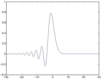
Figure 2: Numerical solutionW⁺to the right going lKdV-problem, evaluated int = 1.

It is obtained with a finite difference scheme for initial data W⁺(x,0) = sech(x) =

2

e^x+e^−x. The solution W⁻ is obtained by symmetry.

Definition 2.4 (The lKdV equations). We distinguish between a right moving and a left moving wave. Denote by W^±(x, t) the unique solution to

∂_tW^±(x, t)± a^∗₂

2c^∗∂_x³W^±(x, t) = 0, W^±(x,0) = c^±₀(x)

for (x, t)∈R×(0, T) and c^±₀ as in (3.1).

The existence and uniqueness as well as energy estimates of a solution are a direct consequence of the results in Ref.[17], see Section 3 for more details. In fact, the weakly dispersive problem and the lKdV problem have strong solutions, which can be explicitly constructed by means of Fourier analysis.

We are now able to state the main one-dimensional results. The first shows that the weakly dispersive problem of Definition 2.3, which is also known as linear Boussinesq equation, provides a good approximation of the original problem.

Theorem 2.5. Let c₀, d₀ ∈ C_c^∞ (−R, R)

and RR

−Rd₀(x)dx = 0. Consider u_ε from the time-scaled homogenization problem of Definition 2.2 and the weakly dispersive solution v_ε of Definition 2.3. Then there exists an ε-independent constantC such that ku_ε(x, t)−v_ε(x, t)k_L^∞_(0,T;L^∞_(R)) ≤Cε. (2.2) We note that in (4.6), (4.7) a slightly stronger convergence is derived. We further remark that in the original time scale, Theorem 2.5 reads as

Remark 2.6. Consider u¯_ε as in Definition 2.1 and v¯_ε the unique solution to the rescaled weakly dispersive problem

∂_τ²v¯_ε(x, τ)−a^∗∂_x²v¯_ε(x, τ)−ε²a^∗₂

a^∗∂_τ²∂_x²v¯_ε(x, τ) = 0,

¯

v_ε(x,0) =c₀(x), ∂_τv¯_ε(x,0) =d₀(x).

Then

k¯u_ε(x, τ)−v¯_ε(x, τ)k_L^∞_{(0,T /ε}²_;L^∞_(R))≤Cε.

The weakly dispersive solution and the lKdV-solution can be compared as follows.

Theorem 2.7. Consider the weakly dispersive solution v_ε of Definition 2.3 and the shifts w^±_ε of the lKdV-solutions of Definition 2.4

w_ε⁺(x, t) : =W⁺

x− c^∗ ε²t, t

, (2.3)

w_ε⁻(x, t) : =W⁻

x+c^∗ ε²t, t

. (2.4)

Then there exists an ε-independent constant C such that k∂xvε(x, t)−∂x w⁺_ε +w_ε⁻

(x, t)k_L^∞_(0,T;L²_(R)) ≤Cε², k∂_tv_ε(x, t)−∂_t w⁺_ε +w_ε⁻

(x, t)k_L^∞_(0,T;L²_(R)) ≤C. (2.5) Moreover,

kv_ε(x, t)− w_ε⁺+w⁻_ε

(x, t)k_L^∞_(0,T;L^∞_(R))≤Cε. (2.6)

Theorem 2.7 provides a comparison between the solution of the weakly dispersive problem and the lKdV-solutions. This result is not surprising, see Ref.[29] in the non- linear case. Similarly, articles such as [7, 30, 6] establish a link between Boussinesq and KdV-equations. Nevertheless, they do not explicitly recover the setting of Theorem 2.7, which will be obtained in Section 3 with a direct argument. We include the theorem for the sake of self-containedness and to give precise estimates. By contrast, the proof of Theorem 2.5 requires more computationally intensive methods and is performed in Section 4.

By applying the triangle inequality to (2.2) and (2.6) one directly obtains the following result.

Corollary 2.8. Consider u_ε from the time-scaled homogenization problem and the lKdV-solutions W^±. Then there exists an ε-independent constant C such that

u_ε(x, t)−W⁺ x− c^∗

ε²t, t

−W⁻ x+ c^∗

ε²t, t

L^∞(0,T;L^∞(R))

≤Cε. (2.7) The corollary suggests that the solution to the time-scaled homogenization problem of Definition 2.2 is approximatively equal to two waves propagating with speed c^∗/ε² in opposite directions. Moreover, it shows that the shape of the right going wave is well described by the solution W⁺ to the lKdV-problem, those of the left going wave by W⁻. Similarly to Remark 2.6, this result provides also an approximation of ¯u_ε in the original time scale.

Remark 2.9. Consider u¯ε as in Definition 2.1 and the lKdV-solutions W^±. Then there exists an ε-independent constant C such that

u¯_ε(x, τ)−W⁺

x−c^∗τ, ε²τ

−W⁻

x+c^∗τ, ε²τ

L^∞(0,T /ε²;L^∞(R))

≤Cε.

2.2 Main results in an abstract framework and the multi- dimensional case

Theorem 2.5 and Corollary 2.8 contain a complete description of the long time behavior of waves in the one-dimensional case. In the multi-dimensional setting, x ∈ R^N, the situation is much more complicated and it seems that, up to now, comparable results or even an effective equation are out of reach.

In the last part of this thesis, Sections 6-8, we will therefore study the multi- dimensional homogenization problem in a more abstract framework. More precisely, we define an energy densityE_ε(ξ, t) and show that a weak star limitµ∈L^∞(0, T;M(R^N)) exists. Based on the one-dimensional results of Sections 3-5 we prove that for N = 1 the energy measure µ is in fact a Dirac measure. For N ≥ 2 the identification of µ remains an open problem. In Section 8 we derive at least restrictions on the support of µ.

Let us now state the N-dimensional long time homogenization problem.

Definition 2.10 (N-dimensional homogenization problem). Let N ∈ N, N ≥ 2 be arbitrary. Let T, R > 0 and let A(·) ∈ C^∞(R^N,R^N×N) be (0,1)^N-periodic. More- over, let A(y) ∈ M(α, β) be symmetric and admissible in the sense of Definition

1.1 for every y ∈ R^N. Let c0, d0 ∈ C_c^∞(BR(0)). We call u¯ε(x, τ) a solution to the N-dimensional long time homogenization problem if u¯_ε ∈ L^∞(0, T /ε²;H²(R^N)),

∂_τu¯_ε ∈L^∞(0, T /ε²;H¹(R^N)) and

∂_τ²u¯ε(x, τ) = ∇ · A

x ε

∇¯uε(x, τ)

, (2.8)

¯

u_ε(x,0) =c₀(x),

∂_tu¯_ε(x,0) =d₀(x).

Analogous to the one-dimensional case, see Definition 2.2, the time-scaled homog- enization problem in N space dimensions reads as follows.

Definition 2.11(Time-scaled homogenization problem inN space dimensions). Con- sider the setting of Definition 2.10. We denote by uε(x, t) the unique solution to

ε⁴∂_t²u_ε(x, t) =∇ · Ax

ε

∇u_ε(x, t) , u_ε(x,0) =c₀(x),

∂_tu_ε(x,0) = 1 ε²d₀(x) for (x, t)∈R^N ×(0, T).

We are now in the position to introduce the N-dimensional energy measureµ and to state the main results in the abstract framework.

Definition 2.12 (Energy density and energy measure). Let N ∈N be arbitrary.

For N = 1let u_ε be the solution to the one-dimensional time-scaled homogenization problem of Definition 2.2. For N ≥ 2 let uε be the solution to the multi-dimensional time-scaled homogenization problem of Definition 2.11.

1. We define the N-dimensional energy density E_ε(ξ, t) by E_ε(ξ, t) := 1

ε^2N

A· ε

∇u_ε(·, t)T

A· ε

∇u_ε(·, t) ξ ε²

. (2.9) 2. We call µ ∈ L^∞(0, T;M(R^N)) an energy measure if there exists a subsequence

E_εk of E_ε such that E_εk * µ^∗ in L^∞(0, T;M(R^N)).

The existence of a weak star limitµis shown in Section 6. It is a direct consequence of the energy estimate for the time-scaled wave equation, which can be found in the appendix.

Remark 2.13. In the one-dimensional case, N = 1, the energy density E_ε of Defini- tion 2.12 is defined through a homogenization problem with well adapted initial data. In this setting, we will use the fine results of Subsection 2.1 to identify the one-dimensional energy measure µ, see (2.10) below.

For non-adapted initial data we can only prove restrictions on the support of µ.

More precisely, the result of Theorem 2.15 below is also valid for the one-dimensional homogenization problem with non-adapted initial data.

In Subsection 6.1 we prove that for N = 1 the energy measureµof Definition 2.12 is in fact a Dirac measure,

µ(ξ, t) =h

(a^∗)²k∂_xc⁺₀k²_L2(R)

i

δ_c^∗_t(ξ) +h

(a^∗)²k∂_xc⁻₀k²_L2(R)

i

δ−c^∗t(ξ), (2.10) where c⁺₀ is the right going part of the initial data and c⁻₀ is the left going part, respectively. Eq. (2.10) reflects the fact that the solution to the one-dimensional long time homogenization problem is approximatively equal to two waves propagating with speed c^∗ in opposite directions. We observe that, unlike Theorem 2.5 and Corollary 2.8, the energy measure µ doesn’t contain any information about the fine properties of the solution.

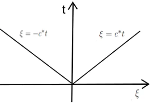
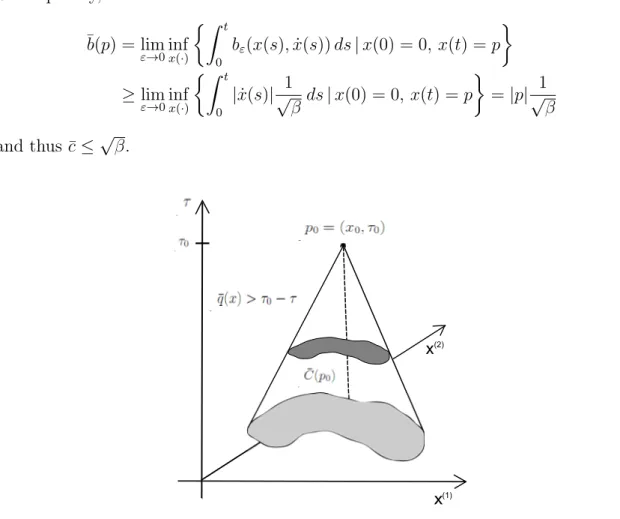
In the multi-dimensional case, N ≥ 2, a rigorous identification of µ seems to be out of reach. In Subsection 7.3 we introduce the notion of effective speeds. More precisely, we define the energetic effective speed cˆthrough the slope of the smallest cone in space-time which contains the support of any energy measure µ. We set

ˆ

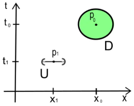
c:= inf{c >0| suppµ⊆C(c) for every energy measureµ}, (2.11) where C(c) denotes the cone with slope ¹_c, C(c) :={(ξ, t)∈R^N ×(0, T)| |ξ| ≤ct}.

Our main result in the multi-dimensional setting is Theorem 2.15 below. It provides an upper bound for the energetic effective speed ˆcin terms of another homogenization problem. To be more precise, we exploit a connection between uε, solution to the multi-dimensional homogenization problem of Definition 2.11, and the Riemannian distanceq_ε according toA _ε^·

.

Definition 2.14 (Riemannian distance). Let N ∈ N be arbitrary. Let A(·) be as in Definition 2.10 and let x0 ∈ R^N be fixed. We define qε(x) as the unique viscosity solution to the Hamilton-Jacobi equation

(∇q_ε)^T(x)Ax ε

∇q_ε(x) = 1, q_ε(x)>0 in R^N \ {x₀}, q_ε(x₀) = 0.

(2.12) In what follows we assume that the matrix A _ε^·

is in fact a scalar function, A _ε^·

= a _ε^·

IdN with IdN denoting the N ×N unit matrix. Due to Proposition 7.7 of Subsection 7.3 the Riemannian distance q_ε converges uniformly on R^N to the effective distance ¯q,

¯

q(x) =|x−x₀|¯b

x−x₀

|x−x₀|

with an effective cost function ¯b. We define the geometric effective speed ¯c as the maximal value of 1/¯b,

¯ c:=

min

|x|=1

¯b(x) −1

. (2.13)

Let us now state the main result in theN-dimensional abstract setting. The proof of Theorem 2.15 is given in Section 8.

Theorem 2.15 (Upper bound for the energetic effective speed). Let N ∈N be arbi- trary. Let ˆcbe the energetic effective speed of (2.11)and let ¯cbe the geometric effective speed of (2.13) Then the following inequality holds

ˆ

c≤¯c. (2.14)

The theorem provides an upper bound for the energetic effective speed ˆcin terms of the effective distance ¯q. However, this bound is not optimal. The non-optimality is shown in Subsection 7.4 using the fine results of the one-dimensional case.

Part II

The one-dimensional case

3 Weakly dispersive equation and the lKdV-problems

This section is devoted to the proof of Theorem 2.7. We will discuss the well-posedness of the lKdV-problem in Subsection 3.1. After some preliminaries in Subsection 3.2, the proof of Theorem 2.7 is given in Subsection 3.3.

3.1 The lKdV-problems and their shifts

Let us start with some preliminaries concerning theleft going and theright going part of the initial data. In fact, due to classical theory, each solution to the one-dimensional wave equation

∂_t²u(x, t)−(c^∗)²∂_x²u(x, t) = 0 is given by

u(x, t) = f(x−c^∗t) +g(x+c^∗t).

In particular,

u(x,0) =f(x) +g(x) and ∂_tu(x,0) =−c^∗∂_xf(x) +c^∗∂_xg(x).

Consequently, the following definition is useful.

Definition 3.1 (Decomposition of the initial data). Let c^∗ >0. We define P_c^+∗(c0, d0) and P_c⁻∗(c₀, d₀) as solutions of

P_c⁺∗(c₀, d₀)

(x) + P_c⁻∗(c₀, d₀)

(x) =c₀(x),

−c^∗∂_x P_c⁺∗(c₀, d₀)

(x) +c^∗∂_x P_c⁻∗(c₀, d₀)

(x) =d₀(x).

In the following, we will use the abbreviationsc⁺₀ :=P_c⁺∗(c₀, d₀) andc⁻₀ :=P_c⁻∗(c₀, d₀).

Remark 3.2. The decomposition of Definition 3.1 satisfies the following properties.

1. The projections c⁺₀, c⁻₀ are uniquely defined up to an additive constant.

2. In the case of smooth initial data, c₀, d₀ ∈C^∞ (−R, R)

, also their projections are smooth, i.e. c⁺₀, c⁻₀ ∈C^∞ (−R, R)

.

3. In the case that c₀, d₀ ∈C_c^∞((−R, R)) with RR

−Rd₀(x)dx = 0, there exist unique compactly supported projections, c⁺₀, c⁻₀ ∈C_c^∞((−R, R)).

We will always work with 3. and have unique projections. In this case c⁺₀(x) = 1

2c₀(x) + 1 2c^∗

Z R x

d₀(ξ)dξ, c⁻₀(x) = 1

2c₀(x)− 1 2c^∗

Z R x

d₀(ξ)dξ.

(3.1)