Friedmann-Robertson-Walker Universe

Chapter 4

Friedmann-Robertson-Walker Universe

To find solutions to the Einstein equations for our Universe, we must first make an Ansatz: what do we think the metric could look like? This brings us to the Robertson- Walker metric, in which certain factors will remain undetermined. To determine these, and to test if the Robertson-Walker Ansatz is good in the first place, we insert this met- ric into the Einstein Equations. This will then prove that the metric is indeed a good Ansatz, and it will lead to constraints on the undetermined factors: The Friedmann Equations. These equations are two simple first order ordinary differential equations.

Solutions to these equations yield the cosmological model we are interested in.

4.1 Robertson-Walker geometry of space

The Universe is homogeneous and isotropic. Isotropy means that the metric must be diagonal. Because, as we shall see, space is allowed to be curved, it will turn out to be useful to use spherical coordinates (r, θ, φ) for describing the metric. The center of the spherical coordinate system is us (the observers) as we look out into the cosmos.

Let us focus on the spatial part of the metric. For flat space the metric is given by the following line element:

ds ² = dr ² + r ² (dθ ² + sin ² θ dφ ² ) (4.1) where θ is now measured from the north pole and is π at the south pole. It is useful to abbreviate the term between brackets as

dω ² = dθ ² + sin ² θ dφ ² (4.2)

because it is a measure of angle on the sky of the observer. Because the universe is isotropic the angle between two galaxies as we see it is in fact the true angle from our vantage point: The expansion of the universe does not change this angle. Therefore we can use dω for the remainder of this lecture. So, for flat space we have

ds ² = dr ² + r ² dω ² (4.3)

It was proven by Robertson and Walker that the only alternative metric that obeys both isotropy and homogeneity is:

ds ² = dr ² + f K (r) ² dω ² (4.4)

where the function f K (r) is the curvature function given by f K (r) =



 

 

 

 

K ^{− 1/2} sin(K ^1/2 r) for K > 0

r for K = 0

K ^{− 1/2} sinh(K ^1/2 r) for K < 0

(4.5)

This means that the circumference of a sphere around us with radius r is, for K ! 0, not anymore equal to C = 2πr but smaller for K > 0 and larger for K < 0. Also the surface area of that sphere is no longer S = (4π/3)r ³ but is smaller for K > 0 and larger for K < 0. For small r (to be precise, for r " | K | ^{− 1/2} ) the deviation from C = 2πr and S = (4π/3)r ³ is small, but as r approaches | K ^{− 1/2} | the deviation can become very large.

This is very similar to the 2-D example of the Earth’s surface. If we stand on the North Pole, and use r as the distance from us along the sphere (i.e. the lattitudinal distance) and dφ as the 2-D version of dω, then the circumference of a circle at r = 10000 km (i.e. the circle is the equator in this case) is “just” 40000 km instead of 2π × 10000 = 62831 km, i.e. a factor of 0.63 smaller than it would be on a flat surface.

The constant K is the curvature constant. We can also define a “radius of curvature”

R curv = K ^{− 1/2} (4.6)

which, for our 2-D example of the Earth’s surface, is the radius of the Earth. In our 3- D Universe it is the radius of a hypothetical (!) 3-D “surface” sphere of a 4-D “sphere”

in 4-D space.

Note that the metric given in Eq. (4.4) can be written in another way if we define an alternative radius r as r ≡ f K (r). The metric is then:

ds ² = d r ²

1 − K r ² + r ² dω ² (4.7)

Note that this metric is different only in the way we choose our coordinate r; it is not in any physical way different from Eq. (4.4).

4.2 Friedmann Equations

We can now build our universe by taking for each point in time a Robertson-Walker (RW) space. We allow the scale factor and the curvature of the RW space to vary with time. This gives the generic metric

ds ² = − dt ² + a(t) ² % dx ² + f K (x) ² x ² dω ² & (4.8) The function a(t) is the scale factor that depends on time and which will describe the expansion (or contraction) of the universe. We use the symbol x instead of r because, as we shall see, the radial coordinate in this form no longer has a meaning as a true distance. Instead, the “true” distance r (though, as we shall see later, “true distance”

can have different definitions) would be r = a(t)x.

The scale factor a(t) is normalized such that at the present time we have by definition a = 1, meaning that today we have r = x.

If we now insert Eq. (4.8) into the Einstein Equations (3.39), then we obtain, after some tedious algebra, two equations:

' a ˙ a

( ²

= 8πG 3 ρ − Kc ²

a ² + Λ

3 (4.9)

¨ a

a = − 4πG 3

) ρ + 3 p

c ²

* + Λ

3 (4.10)

where the first equation is from the 00 component of the Einstein equations and the second is from the ii component. These are the Friedmann Equations. The nice thing is that after all the hard work we obtain, finally, a very simple set of ordinary differen- tial equations.

The two Friedmann Equations can be combined to yield the adiabatic equation:

d

dt (ρa ³ c ² ) + p d

dt (a ³ ) = 0 (4.11)

which is the relativistic version of the first law of thermodynamics: T dS = dE +pdV = 0, if (as is reasonably well valid for the universe) the entropy is constant. One can see this by taking the time derivative of Eq. (4.9) and using Eq. (4.11) to arrive at Eq. (4.9).

Usually people only use the first Friedmann equation plus an equation of state (i.e.

an integral of Eq. 4.11, see Section 4.4), and thus do not need the second Friedmann equation. This makes all equations first order, which is easier to handle.

4.3 Relation to the Newtonian Universe

Note that the second Friedmann equation, Eq. (4.10), is the GR version of Eq. (2.37) for the Newtonian Universe. You can see this by assuming that p " ρc ² (which is valid for non-relativistic matter) and multiplying Eq. (4.10) by ax. If we identify R(t) = xa(t) we obtain

R ¨ = − GM R ² + Λ

3 R (4.12)

which is identical to Eq. (2.37).

The first Friedmann equation, Eq. (4.9), is the GR version of the energy budget equa- tion. If we multiply it with ¹ ₂ a ² x ² we obtain

1

2 R ˙ ² = GM R + Λ

6 R ² − 1

2 Kc ² x ² (4.13)

If we follow a parcel of gas at location R and put Λ = 0, then the terms of this equation have the following meaning:

E kinetic = E grav − E missing (4.14)

where E kinetic = R ˙ ² /2 is the kinetic energy per gram of gas of the parcel, E grav = GM/R is the gravitational potential energy per gram and E missing = Kc ² x ² /2 is the missing kinetic energy for gravitational escape. If K > 0 then E kinetic < E grav and the expansion is subcritical, i.e. the universe will collapse again; If K < 0 then E kinetic > E grav and the universe will expand.

4.4 Scaling of relativistic and non-relativistic matter

Let us have a closer look at the adiabatic equation Eq. (4.11). Note that this equation is strictly speaking only valid if no entropy is generated, but it turns out to be a good approximation.

Let us look at the limiting case of cold matter, i.e. matter for which the pressure p " ρc ² (for cold matter) (4.15) In that case Eq. (4.11) reduces to

d

dt (ρa ³ ) = 0 (4.16)

which means that the equation of state for such cold matter is ρ ∝ 1

a ³ (for cold matter) (4.17)

If we look at the other limiting case, of ultrarelativistic matter, we have the maximum possible relativistic isotropic pressure, which is

p = ρc ²

3 (for ultra-hot matter, radiation) (4.18)

Neutrinos are expected to have velocities very close to the light speed, so that they obey Eq. (4.18). Photons have exactly the light speed, so they obey Eq. (4.18) exactly.

Eq. (4.11) now reduces to d

dt (ρa ³ c ² ) + ρc ² 3

d

dt (a ³ ) = 0 (4.19)

which works out to ρ ∝ 1

a ⁴ (for ultra-hot matter, radiation) (4.20) We will assume, from now on, that there exists only cold matter and radiation in our universe, so nothing in between.

4.5 The Critical Density, and the dimensionless Friedmann equa- tion

4.5.1 The critical density

In Chapter 2 we already realized that there is a critical expansion velocity, for any given density of the universe. Observationally, however, we tend to know the expan- sion velocity of the Universe at the present time (i.e. the Hubble constant), but it is much harder to measure the density of the Universe, because as we know, much of the matter is dark. So the critical velocity in fact turns into a critical density. The way to define this is to start from the first Friedmann equation, Eq. (4.9) and write it in the following form:

H ² = 8πG 3

+ ρ + ρ Λ ,

− Kc ²

a ² (4.21)

with the Hubble “constant” H = a/a, and we wrote ˙ Λ as ρ Λ according to:

ρ Λ ≡ Λ

8πG (4.22)

The density ρ can be written as contributions from “matter” (baryons and cold dark matter) and “radiation”:

ρ = ρ m + ρ r (4.23)

We can go even further, by writing the matter density as baryonic matter and cold dark matter:

ρ m = ρ b + ρ cdm (4.24)

and by writing the radiation as consisting of photons and neutrinos:

ρ _r = ρ _γ + ρ _ν (4.25)

But for the moment we will keep ρ _m and ρ _r because for their scaling with a the ρ _b and ρ _cdm behave identically, and so do ρ _γ and ρ _ν . The first Friedmann equation then becomes:

H ² = 8πG 3

+ ρ _m + ρ _r + ρ Λ ,

− Kc ²

a ² (4.26)

If we define the critical density ρ _crit as

ρ crit = 3H ²

8πG (4.27)

then we see that if the total density ρ m + ρ r + ρ Λ equals the critical density, then K = 0,

meaning that the universe is flat. By the equivalence of curvature and expansion rate

this also means that the universe expands critically. The critical density is therefore

the density at which the universe expands critically, given the value for H.

4.5.2 Dimensionless Friedmann equation

If we define H 0 as the Hubble “constant” at the present time and ρ crit,0 as the critical density at the present time, then the first Friedmann equation becomes:

H ² = H ₀ ² ) ρ m

ρ crit,0

+ ρ r

ρ crit,0

+ ρ Λ

ρ crit,0

*

− Kc ²

a ² (4.28)

At this point it is convenient to introduce the following dimensionless densities:

Ω _m (a) = ρ m (a)

ρ _crit (a) (4.29)

Ω _r (a) = ρ _r (a)

ρ crit (a) (4.30)

Ω Λ (a) = ρ Λ (a)

ρ _crit (a) (4.31)

The values of these quantities at the present time are denoted as Ω m,0 , Ω r,0 and Ω Λ,0 . It is convenient to introduce Ω _K (a), resp. Ω _K,0 at this point. If we consider the first Friedmann equation at the present time:

H ₀ ² = H ² ₀ + Ω m,0 + Ω r,0 + Ω Λ,0 ,

− Kc ² (4.32)

we can evaluate the curvature in terms of H 0 , Ω m,0 , Ω r,0 and Ω Λ,0 :

Kc ² = H ² ₀ + Ω _m,0 + Ω _r,0 + Ω _Λ,0 − 1 , (4.33) So if we define the “curvature density” Ω _K,0 :

Ω K,0 ≡ − Kc ²

H ₀ ² = 1 − Ω m,0 − Ω r,0 − Ω Λ,0 (4.34) we get that all Ωs add up to 1. In analogy to Eqs. (4.29, 4.30, 4.31) we can define Ω K (a) in terms of a “curvature density”:

Ω _K (a) = ρ _K (a)

ρ crit (a) (4.35)

The Ω symbols can be used to rewrite the Friedmann equation. For this, we must know the equations of state of matter and radiation. We already discussed them in Section 4.4: The matter density goes as 1/a ³ . Radiation as 1/a ⁴ . The Ω _Λ stays constant. The Ω _K goes, according to Eq. (4.34), as 1/a ² . So we can write:

H ² = H ² ₀ ) Ω _m,0

a ³ + Ω _r,0

a ⁴ + Ω Λ,0 + Ω _K,0 a ²

*

= H ² ₀ E ² (a)

(4.36)

(note that at the present time a = 1). This is the form of the Friedmann equation that is usually used, because it contains essentially all the information we need. If we have measured H 0 we can calculate ρ _crit,0 via Eq. (4.27). We must then measure ρ _m,0 , ρ r,0 and Λ from which we directly obtain Ω m,0 , Ω r,0 and Ω Λ,0 . The Ω K,0 then follows immediately from Eq. (4.34). We now have an equation (Eq. 4.36) that is fully self contained, and we can (numerically or analytically) integrate it to get the evolution of the universe.

4.5.3 Behavior of Ω _m , Ω _r , Ω Λ and Ω _K as a function of a

In Eq. (4.36) we expressed the Friedmann equation in terms of the Ω-values and the

Hubble constant as they are at the present time. But sometimes it is useful to also

know how the values of Ω _m (a), Ω _r (a), Ω Λ (a) and Ω _K (a) behave for a ! 0. Although Eq. (4.36) appears to suggest that e.g. Ω m (a) ∝ 1/a ³ , this is not the case! The 1/a ³ behavior of the first term in Eq. (4.36) is because the entire part between brackets is multiplied by H ₀ ² , not by H ² . So indeed, for a ! 1

Ω m,0

a ³ + Ω r,0

a ⁴ + Ω _Λ,0 + Ω K,0

a ² ! 1 for a ! 1 (4.37)

But by the definition of the Ωs in Eqs. (4.29, 4.30, 4.31, 4.35) we have at all times (i.e.

for all values of a):

Ω _m (a) + Ω _r (a) + Ω Λ (a) + Ω _K (a) = 1 (4.38) This means that the behaviors of Ω m (a), Ω r (a), Ω Λ (a) and Ω K (a) are somewhat com- plex.

As an example let us work out the behavior of Ω _m,0 and Ω _Λ,0 in a Universe with Ω _K = 0 and Ω _r = 0. We have

Ω _m (a) = ρ m (a)

ρ _crit (a) and Ω Λ (a) = Λ

ρ _crit (a) (4.39) We know that Λ is constant in time and we know that

ρ m (a) = ρ _m,0

a ³ (4.40)

We also know that

Ω m (a) + Ω Λ (a) = 1 (4.41)

which leads to

ρ _m,0

a ³ ρ _crit (a) + Λ

ρ crit (a) = 1 (4.42)

With this equation we can express ρ crit (a) as ρ crit (a) = ρ _m,0

a ³ + Λ (4.43)

which leads to

Ω m (a) = ρ m,0

a ³ 1

ρ

a

+ Λ (4.44)

Ω Λ (a) = Λ 1

ρ

a

+ Λ (4.45)

Equivalently, you can also express these in terms of Ω _m,0 and Ω _Λ,0 : Ω _m (a) = Ω _m,0

a + Ω _m,0 (1 − a) + Ω _Λ,0 (a ³ − a) (4.46) Ω Λ (a) = Ω _Λ,0 a ³

a + Ω _m,0 (1 − a) + Ω _Λ,0 (a ³ − a) (4.47) Just keep in mind that these equations only hold when Ω r = Ω K = 0 (or if these values are very small).

4.6 Simple Universe Models

If the Universe were to consist of only one of the four kinds of “matter” in Eq. (4.36)

then it is easy to integrate the Friedmann equation analytically. Let us do this here.

4.6.1 Matter-dominated Flat Universe

If Ω m,0 = 1 and Ω r,0 = Ω Λ,0 = Ω K,0 = 0 then Eq. (4.36) becomes

˙ a

a = H 0 1

a ^3/2 (4.48)

which has as a solution (with a = 0 at the time of the Big Bang t = 0):

t = 2a ^3/2

3H 0 ↔ a(t) =

) 3 2 H 0 t

* 2/3

(4.49) This is an expanding Universe in which the expansion rate is inversely proportional to time: H(t) = 2/3t, i.e. it is a decellerating Universe. According to this model the age of the Universe would be t = 2/3H 0 which amounts to 9.26 × 10 ⁹ years. This is the Einstein-de Sitter model of the Universe.

4.6.2 Radiation-dominated Flat Universe

If Ω _r,0 = 1 and Ω _m,0 = Ω _Λ,0 = Ω _K,0 = 0 then Eq. (4.36) becomes

˙ a a = H 0

1

a ² (4.50)

which has as a solution (with a = 0 at t = 0):

t = a ²

2H 0 ↔ a(t) = (2H 0 t) ^1/2 (4.51)

Like the matter-dominated Universe the radiation-dominated Universe expands but decellerates: H(t) = 1/2t. The age of the Universe would be t = 1/2H 0 which amounts to 6.94 × 10 ⁹ years.

This demonstrates a peculiar phenomenon: Pressure apparently does not help to coun- teract the decelleration due to gravity, as one would perhaps think. The reason is that only a pressure gradient can induce a force. Since there is no pressure gradient in a ho- mogeneous Universe, pressure cannot help expand the universe. Instead: matter with pressure is even more effective at decellerating the Universe than cold matter. This is because in addition to ρ there is also an additonal 3p/c ² in the second Friedmann equation, Eq. (4.10). This is a purely relativistic effect.

4.6.3 Λ-dominated Flat Universe

If Ω _Λ,0 = 1 and Ω _m,0 = Ω _r,0 = Ω _K,0 = 0 then Eq. (4.36) becomes

˙ a

a = H 0 (4.52)

This does not have a solution that obeys a = 0 at t = 0. Instead it produces an exponentially expanding Universe:

a(t) = e ^H

^t (4.53)

where in this case we take t = 0 to be today. The age of the Universe is infinite, in this case.

4.6.4 Empty Universe

If the Universe would have a matter content that is very much smaller than the critical density, we can approximate Ω _m,0 ' Ω _r,0 ' Ω _Λ,0 ' 0 and we have Ω _K,0 ' 1. Then Eq. (4.36) becomes

˙ a a = H 0

a (4.54)

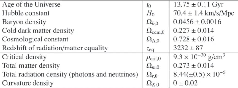
Age of the Universe t 0 13.75 ± 0.11 Gyr

Hubble constant H 0 70.4 ± 1.4 km/s/Mpc

Baryon density Ω _b,0 0.0456 ± 0.0016

Cold dark matter density Ω _cdm,0 0.227 ± 0.014

Cosmological constant Ω Λ,0 0.728 ± 0.016

Redshift of radiation/matter equality z eq 3232 ± 87

Critical density ρ crit,0 9.3 × 10 ^{− 30} g/cm ³

Total matter density Ω _m,0 0.273 ± 0.014

Total radiation density (photons and neutrinos) Ω _r,0 8.44( ± 0.5) × 10 ^{− 5}

Curvature density Ω _K,0 0 ± 0.02

Table 4.1: Cosmological constants derived from 7 years of WMAP, from Jarosik et al. (2011, ApJS 192, 14). Used here is the “WMAP+BAO+H 0 ” column of table 8 of that paper. Everything below the line is derived from the parameters above the line. Equations used are Ω m,0 = Ω b,0 + Ω cdm,0 , Ω r,0 = Ω m,0 /(1 + z eq ) and Ω K,0 = 1 − Ω m,0 − Ω r,0 − Ω Λ,0 . Note that Ω b,0 = ρ b,0 /ρ crit,0 and Ω cdm,0 = ρ cdm,0 /ρ crit,0 . which has as a solution (with a = 0 at t = 0):

a(t) = H 0 t (4.55)

This is a Universe in which everything is moving ballistically away from us with a constant velocity. The age of the Universe is then identical to the Hubble time, i.e. t = 1/H 0 which is 1.39 × 10 ¹⁰ years. The Universe is then not flat anymore.

The constant of curvature K is then K = − 5.8 × 10 ^{− 57} cm ^{− 2} which gives a radius of curvature of R curv = 4.26 × 10 ⁹ parsec.

4.7 The Standard Model of the Universe

The current paradigm is that the Universe is flat Ω K,0 ' 0, but contains matter, radia- tion and has a non-zero cosmological constant. The latter is presumably a consequence of so-called dark energy (more on that later in this lecture). In table 4.1 the parameters of this standard model are listed.

One can see that we are currently dominated by Λ by a factor of three. This means that we are now in a phase of exponential growth! But before about z ! 0.5 the Universe was dominated by cold matter, and before about z ! 3200 the Universe was dominated by radiation.

The integration of Eq. (4.36) with three of four terms non-zero is, unfortunately, not possible analytically. A numerical integration is required. But for the radiation- dominated phase and for the matter-dominated phase of the Universe we can use (adapted versions of) the solutions of Section 4.6 as an approximation. So, for the early radiation-dominated phase we approximate the solution by

a(t) ' - 2H 0

. Ω _r,0 t / 1/2

(radiation-dominated era) (4.56) The .

Ω _r,0 factor comes in because if we insert a " 10 ^{− 4} into Eq. (4.36) the other three terms vanish, but the factor Ω _r,0 remains. The early radiation-dominated Universe expanded as a ∝ √

t.

Likewise, for the matter-dominated era we get approximately a(t) '

) 3 2 H 0

. Ω _m,0 t

* 2/3

(matter-dominated era) (4.57)

The later matter-dominated Universe expanded as a ∝ t ^2/3 .

The transition from the radiation-dominated era to the matter-dominated era occurs when Ω m,0 /a ³ = Ω r,0 /a ⁴ , which is at a = 0.00031. Inserting this into Eq. (4.56) yields a time of roughly 7 × 10 ⁴ years after the Big Bang.

The late Universe (z =few until z = 0), in which both matter and Λ are important but radiation is unimportant, can also be integrated analytically. This is fortunate because it is during this period that most of the structure formation in the Universe occurs (as we shall discuss later), and it is the era which we can most readily observe. So let us take 0 < Ω _m,0 < 1 and Ω _Λ,0 = 1 − Ω _m,0 , and set Ω _r,0 = 0 and Ω _K,0 = 0. Eq. (4.36) then becomes

1 a

da dt = H 0

0 Ω m,0

a ³ + Ω _Λ,0 (4.58)

which can be integrated as t = 1

H 0

1 a

0

da ⁾ a ⁾ .

Ω _m,0 /a ^{) 3} + Ω _Λ,0 = 1 H 0

1 a

0

√ a ⁾ da ⁾

. Ω _m,0 + Ω _Λ,0 a ^{) 3} (4.59) By substituting x = a ^3/2 this can be integrated to

t = 2

3H 0 .

1 − Ω _m,0 arcsinh



 

 

 



5 1 − Ω _m,0 Ω m,0

a ^3/2



 

 

 



(4.60) One can verify that for small a this formula approaches Eq. (4.57) and that for a * 1 (i.e. far into the future) this formula describes an exponentially expanding Universe.

Eq. (4.60) is very accurate for all redshifts up to, say, z ' 1000. That means that we can also use it to accurately estimate the age of the Universe: we simply insert a = 1 into Eq. (4.60) and we obtain, with Ω _m,0 = 0.273 an age of 13.7 Gyr.

4.8 Light propagation through the Universe

If we observe a galaxy at some redshift z, we may want to know how the light has moved through the Universe from that galaxy to us. This is not a trivial question because the light moves through the Universe while the Universe is expanding. Let us try to calculate the coordinate distance (comoving distance) of that galaxy as a function of its redshift:

x(z) = 1 x(z)

0

dx = − 1 t

t(z)

) dx dt

* dt = −

1 1 a(z)

) dx dt

* ) dt da

*

da (4.61)

We know what a(z) is: a(z) = 1/(1 + z). We also know that for light propagating toward us

dx dt = − dx

dr dr dt = c

a (4.62)

We thus obtain

x(z) = 1 1

a(z)

cda

a a ˙ (4.63)

With Eq. (4.36) we can eliminate ˙ a in favor of E(a):

x(z) = c H 0

1 1 a(z)

da

a ² E(a) (4.64)

We can numerically integrate this for a general universe. Note that if we replace

the integration domain with arbitrary a start and a finish we can calculate the δx of light

propagation between a start and a finish .

4.9 Distances

In an expanding Universe it is not trivial to define distances. We will define several different kinds of distance here. Since all the current evidence today points to a flat universe, we will assume a flat universe from now on. We will be interested to measure the distance of some object at redshift z to us (redshift z = 0).

4.9.1 Comoving distance D com

The comoving distance to some object at coordinate distance x is the spatial distance within a t =const spatial hypersurface:

D com (x, t) = r(t) = a(t)x (4.65) This is the intuitive way of defining distance, but it is not directly measurable, because light does not travel at infinite speed. Also, we typically measure the redshift of the object, so instead of D com (x, t) we would like to know D com (z, t). If we take the current time (a = 1) then we can use Eq. (4.64) and obtain

D com (z) = x(z) = c H 0

1 1 a(z)

da

a ² E(a) (4.66)

The comoving distance to the Big Bang (excluding inflation) can be obtained by nu- merical evaluation of Eq. (4.66) with a(z) = 0. This yields D com (z → ∞ ) = 1.43 × 10 ¹⁰ parsec, which is about 3.37 times r H .

4.9.2 Proper distance D prop

The proper distance to some object is the distance measured by the time it takes for light from that object to reach us. Analogous to Eq. (4.61) we write the time t(z) when the light was emitted as an integral between t(z) and the present time t 0 :

t(z) = t 0 − 1 t

t(z)

dt = t 0 − 1 1

a(z)

) dt da

*

da = t 0 − 1 1

a(z)

da

˙ a

= t 0 − 1 H 0

1 1 a(z)

da aE(a)

(4.67)

The distance is then

D prop (z) = c(t 0 − t(z)) = c H 0

1 1 a(z)

da

aE(a) (4.68)

Note that for the late universe (z " 1000) in which only cold matter and Λ dominate, this integral happens to be very similar to the integral of Eq.(4.59) for the age of the universe. So the analytical solution for z " 1000 is

D prop (z) = 2 3 .

1 − Ω _m,0



 

 

 

 arcsinh



 

 

 



5 1 − Ω _m,0 Ω m,0



 

 

 

 − arcsinh



 

 

 



5 1 − Ω _m,0 Ω m,0 a(z) ^3/2



 

 

 





 

 

 

 (4.69)

4.9.3 Angular distance D ang

In a non-expanding flat space the distance to some galaxy can be estimated from the angular size ∆ω on the sky, if we know what the true diameter S in units of centimeters of the galaxy is. Since ∆ω " 1 we can then write

D ang = S

∆ω (4.70)

We define the angular distance D ang with Eq. (4.70) even when the Universe expands, i.e. it is the distance that the galaxy would have if the universe were static.

If we do not know the true size S and/or if we can not spatially resolve the angular size ∆ω on the sky, then we need to determine D ang using the redshift z. To do this let us first compute what ∆ω would be of a “galaxy” that is gravitationally unbound, i.e.

a “galaxy” for which the size S (t) scales linearly with a(t). The solid angle ∆ω that that object has on the sky would then be completely independent of time: In 10 billion years it would still have the same solid angle on our sky. In that case we can, in the spatial hypersurface of today (t = t 0 ), relate S (t 0 ) to ∆ω via the comoving distance D com (t 0 ) via

D com (t 0 , z) = S (t 0 )

∆ω (4.71)

where we assume here that the Universe is flat. Now, with our assumption that S (t) ∝ a(t) we can replace S (t 0 ) with S (t i ) (where t i is the time when the light was emitted):

S (t i ) = a(t i )S (t 0 ) = a(z)S (t 0 ) (4.72) where S (t i ) is the size of the galaxy when the light was emitted. Eq. (4.71) then becomes

D com (t 0 , z) = S (t i )

a(z)∆ω (4.73)

Now we have eliminated any reference to the time-evolution of the galaxy size S (t).

Only the size of the galaxy at the time of emitting its radiation is relevant here.

Eq. (4.73) therefore also holds if the galaxy stays the same size or merely changes size very slowly (which is, of course, a much more realistic assumption). If we define the size S as S := S (t i ) and D com (z) := D com (t 0 , z) (as we did in Section 4.9.1) then Eqs. (4.73, 4.70) can be combined to give:

D ang (z) = a(z)D com (z) (4.74) We can use Eq. (4.74) also to compute the size S if we measure its angular size ∆ω and redshift z.

Note that around z ' 1.5 the angular distance D ang (z) reaches a maximum and then decreases again. This means that if we take a galaxy of given size S and we put it at increasing distance z, then before z ' 1.5 its angular size ∆ω decreases as expected, but beyond z ' 1.5 its angular size increases again!

4.9.4 Luminosity distance D lum

Analogously to the angular distance, we can also make a luminosity distance, defined as if the space were static and euclidian. The observed flux F of a galaxy with surface brightness B, surface area A at a distance D in Euclinian space is

F = BΩ = B A

D ² (4.75)

where Ω = A/D ² is the solid angle of the galaxy on the sky.

In an expanding Universe, however, the brightness B is diluted due to redshift (giving a factor of a), due to the scaling of the surface area of the camera (giving a factor of a ² ) and due to the reduction of the rate of arrival of photons (giving a factor of a).

This means that the flux F we observe today from a galaxy at redshift z is related to the brightness of the galaxy in the past by the following relation:

F = a(z) ⁴ BΩ = a(z) ⁴ B A D ² ang

(4.76)

where B is the brightness of the galaxy at the time it emitted its radiation. The symbol Ω is the solid angle of the galaxy as we observe it today, so we use Ω = A/D ² _ang . If we use Eq. (4.75) as the definition of D lum we then obtain

D lum (z) = 1

a(z) ² D ang (4.77)

So the luminosity distance tends to be much larger than the angular distance because the galaxy becomes extremely dim at large redshift. Eq. (4.77) is called the “Ether- ington relation” and is valid very generally, also for non-flat universes.

4.9.5 Distances in the low-redshift Universe For z " 1 all four distance measures converge to

D lum (z) ' D ang (z) ' D com (z) ' D prop (z) ' cz H 0

+ O (z ² ) (4.78)

4.10 Horizons

From Eq. (4.59) we can see that the Universe has a definite age. That means that there is also a maximum distance that light could have travelled during that time: ct age . More importantly, it means that light could have travelled also only a finite coordinate (comoving) distance x max , given by Eq. (4.64) with a(z) = 0. Any light emitted in the part of the Universe beyond the coordinate distance x max can not yet have reached us.

It is so-to-speak behind the particle horizon.

Let us verify this for the early Universe. As t → 0 and a → 0 the only term in Eq. (4.36) that survives is the radiation term. But let us be more general, and take Ω 0 /a ⁿ instead of Ω r,0 /a ⁴ . So we obtain

E(a) =

√ Ω ₀

a ^n/2 (4.79)

Inserting this into Eq. (4.66) for the comoving distance we obtain D com (z → ∞ ) = c

H 0 √ Ω 0

1 1 0

da

a ^{2 − n/2} = c(n/2 − 1) ^{− 1} H 0 √

Ω 0

? a ^{n/2 − 1} @ 1

0 (4.80)

For n > 2 this converges to a finite number:

D com (z → ∞ ) = c(n/2 − 1) ^{− 1} H 0 √

Ω 0

(4.81) which is the particle horizon. This is the case for our Universe, as the Early universe is radiation-dominated, i.e. n = 4. For n ≤ 2 this integral diverges, meaning that there is no horizon ¹ .

The particle horizon expands with the light speed, so more and more of the Universe becomes visible as time goes by. Unless, however, the Universe expands so fast that this counter-acts this expansion of the particle horizon. To verify if this can happen, let us again take a general powerlaw equation of state (i.e. Ω 0 /a ⁿ ) and calculate the D com from today into the infinite future a → ∞ :

D com (a → ∞ ) = c H 0 √

Ω ₀ 1 1

∞

da

a ^{2 − n/2} = − c(n/2 − 1) ^{− 1} H 0 √

Ω ₀

? a ^{n/2 − 1} @ _∞

1 (4.82)

1

Note the interesting fact that for 0 < n < 2 the comoving distance to the horizon D

(z → ∞) diverges

(i.e. there is no horizon), but the proper distance D

(z → ∞) is finite, i.e. the age of the Universe is finite.

Note that this is negative, because it is a distance into the future. For n < 2 this converges to a finite number:

D com (a → ∞ ) = − c(1 − n/2) ^{− 1} H 0 √

Ω ₀ (4.83)

meaning that any light that we send out today will only ever be seen by a finite portion of the universe. Conversely: only the light that is sent out today by galaxies within this distance will ever be seen by us. This is called the event horizon.

As we discussed before: we are currently in transition from a matter-dominated Uni- verse to a Λ-dominated Universe, with the Λ already dominating over matter by a factor of about 3. This will only get worse in the future, meaning that we are entering an era of exponential expansion, i.e. with n = 0. This means that there is an event horizon for our future Universe.

Note also that for an exponentially expanding Universe, the distance to this event

horizon remains constant in time, even though the Universe expands. This means that

galaxies that are now inside this event horizon will eventually pass through the event

horizon and they will then be effectively out of sight forever.