Testing equality of spectral densities

HOLGER DETTE AND EFSTATHIOS PAPARODITIS

Abstract. We develop a test of the hypothesis that the spectral densities of a number m, m ≥ 2, not necessarily independent time series are equal. The test proposed is based on an appropriate L

-distance measure between the nonpara- metrically estimated individual spectral densities and an overall, ’pooled’ spectral density, the later being obtained using the whole set of m time series considered.

The limiting distribution of the test statistic under the null hypothesis of equal spectral densities is derived and a novel frequency domain bootstrap method is presented in order to approximate more accurately this distribution. The as- ymptotic distribution of the test and its power properties for fixed alternatives are investigated. Some simulations are presented and a real-life data example is discussed.

1. Introduction

A problem that commonly arises in many situations is that of comparing the en- tire autocovariance structure of several, commonly not independent, time series.

Related problems arise in many disciplines like economics, biology, chemistry, etc.

Comparison of the entire autocovariance structure of a number of time series can be effectively done in the frequency domain by comparing their spectral characteristics.

In this context frequency domain methods are appealing and related procedures have been proposed by some authors.

Jenkins (1961) was one of the early attempts, De Souza and Thomson (1982) use an autoregressive model-fitting approach, Shumway (1982) considers similar problems related to discriminant analysis of time series. Coates and Diggle (1986) compare the spectral densities of two independent time series using periodogram based test statistics while Swanepoel and van Wyk (1986) consider two independent stationary

Date: August 17, 2007.

2000 Mathematics Subject Classification. Primary 62M10, 62M15; secondary 62G09.

Key words and phrases. Periodogram, Bootstrap, Multiple time series, Nonparametric kernel estimation, Spectral density matrix.

1

autoregressive processes and use different test statistics and a parametric, autore- gressive bootstrap approach to obtain critical values. Diggle and Fisher (1991) use graphical devices to compare periodograms and apply Kolmogorov-Smirnov or Cramer-von Mises type test statistics based on empirical spectral distributions. Guo (1999) considers first order autoregressions, Timmer et al. (1999) concentrate on spectral peaks and Maharaj (2002) compares evolutionary spectra of non-stationary processes using randomization tests. A test for homogeneity of autoregressive pro- cesses has been also considered by G´omez and Drouiche (2002). However, all ap- proaches proposed so far, suffer from at least one of the following three drawbacks:

They assume that the time series considered are uncorrelated respectively inde- pendent, they impose some parametric, commonly autoregressive structure on the underlying process class and the analysis is restricted to bivariate processes using test statistics generalizations of which to more than two time series are not straight- forward.

In this paper a novel procedure is proposed to test the hypothesis that the second order structure of m, m ≥ 2, time series is identical which overcomes the aforemen- tioned drawbacks of the methods proposed so far. Our approach uses an appropriate L

-type distance measure to evaluate over all frequencies the distance between the nonparametrically estimated spectral density of each individual time series and an estimated, pooled spectral density, the later being obtained using the whole set of m time series at hand. In contrast to common practice in the literature, our testing methodology does not rely on parametric assumptions on the underlying process class nor it assumes that the m time series are uncorrelated respectively indepen- dent. Although the later assumption seems to be convenient from a technical point of view, it largely restricts the applicability of the methods proposed, since in many situations independence of the time series considered can be hardly justified. Under quite general assumptions on the underlying process class, we show that if the null hypothesis of equal spectral densities is true, then the basic test statistic proposed converges weakly to a Gaussian distribution the parameters of which depend in a complicated way on the entire cross-correlation structure of the m dimensional pro- cess. As a special case of our analysis we obtain the limiting distribution of the same test statistic when the time series considered are uncorrelated. In order to improve upon the large sample Gaussian approximation of the distribution of the test statistic under the null, a nonparametric frequency domain bootstrap approach is proposed and its asymptotic validity is established. Furthermore, the power be- havior of the test is investigated and its limiting distribution under fixed alternatives is derived.

The paper is organized as follows. Section 2 states the main assumptions imposed on

the m-dimensional process considered and introduces the basic test statistic used to

test the null hypothesis of equal spectral densities. Section 3 deals with the behavior

of the test statistic under the null. Its asymptotic distribution is derived and the frequency domain bootstrap method is presented and theoretically justified. Section 4 deals with the power properties of the test and derives its asymptotic distribution under fixed alternatives. In Section 5 a small simulation study is presented which investigates the behavior of our testing procedure in final sample situations. Fur- thermore, a real-life data set is analyzed which demonstrates the capability of our testing methodology to detect differences between spectral densities. All proofs are deferred to Section 6.

2. Basic Assumptions and Statistics

Consider a m-dimensional, zero mean second order stationary stochastic process {X

= (X

, X

, . . . , X

)

, t ∈ Z} where m ≥ 2 and assume that

Assumption 1: The random vectors X

have real components and are generated by the equation

X

= X

j=−∞

Ψ

ε

,

where {Ψ

= (ψ

(r, s))

, j ∈ Z} is a sequence of matrices the components of which satisfy

X

j

|j|

|ψ

(r, s)| < ∞, r, s = 1, 2, . . . , m

and {ε

= (ε

, ε

, . . . , ε

)

, t ∈ Z} is a m-dimensional i.i.d. process with mean zero, covariance matrix Σ = (σ

)

> 0 and E[ε

] < ∞, r = 1, 2, . . . , m.

Under Assumption 1, the sequence of covariance matrices {Γ(k), k ∈ Z}, Γ(k) = E(X

X

), has absolutely summable components and the spectral density matrix f (λ) = (f

(λ))

, λ ∈ [−π, π], of {X

, t ∈ Z} exists and is given by

f (λ) = 1 2π

X

k

Γ(k)e

.

Denote by f

(λ) the spectral density of the r-th component of the m-dimensional process, that is the r-th element f

(λ) on the main diagonal of the matrix f (λ).

For the spectral densities f

(λ) of the component series we assume that they fulfill the following condition.

Assumption 2: min

inf

f

(λ) > 0.

Suppose that we have n, n ∈ N, observations of every component of the underlying

process, i.e., suppose that we observe X

, X

, . . . , X

for every r ∈ {1, 2, . . . , m}.

The problem considered is this paper is that of testing H

: f

= f

= · · · = f

, a.e. in [−π, π], vs.

(2.1)

H

: f

6= f

for at least one pair (r, s), r 6= s, and on a set of frequencies Λ ⊂ [−π, π] with positive Lebesque measure.

To derive the statistic for testing hypotheses (2.1) we consider the periodogram matrix I

(λ) = (I

(λ))

where

I

(λ) = J

(λ)J

(λ), and J

(λ) = 1

√ 2πn X

t=1

X

e

.

Here and in the sequel, denotes transposition combined with complex conjugation.

I

(λ) is usually calculated at the Fourier frequencies λ

= 2πj/n, j = −[(n − 1)/2], . . . , [n/2]. Write I

(λ) for the r-th element I

(λ) on the main diagonal of I

(λ) which corresponds to the periodogram of the r-th time series X

, t = 1, 2, . . . , n.

For λ ∈ [−π, π] consider the kernel estimator f b

(λ) of the spectral density f

(λ) defined by

(2.2) f b

(λ) = 1

n X

j∈Z

K

(λ − λ

)I

(λ

),

where K

(·) = h

K(·/h), K is the smoothing kernel and h the smoothing band- width.

Assumption 3: K is a real-valued, 2π-periodic and symmetric kernel satisfying R K

(x)dx < ∞ and R

K(x)dx = 1. We assume that K has a bounded first de- rivative and that for all ω ∈ [−π, π], K(ω) = (2π)

R

−∞

k(u)e

du, where the continuous function k(·) satisfies k(0) = 1 and k(u) = 0 for |u| > 1.

Assumption 4: h → 0 as n → ∞ such that h ∼ n

for some 0 < ν < 2/7.

Let N = mn and consider the pooled kernel estimator w(λ) defined for b λ ∈ [−π, π], by

b

w(λ) = 1 N

X

r=1

X

j∈Z

K

(λ − λ

)I

(λ

).

(2.3)

Standard calculations yield under Assumptions 1, 3 and 4 that E[ w(λ)] = b 1

N X

r=1

X

j∈Z

K

(λ − λ

)(f

(λ

) + O(log(n)n

))

= 1 m

X

r=1

f

(λ) + O(h

+ log(n)n

)

→ w(λ) ≡ 1 m

X

r=1

f

(λ) and

Var[ w(λ)] = b 1 m

n

X

r1,r2

X

j1,j2

K

(λ − λ

)K

(λ − λ

)Cov(I

(λ

), I

(λ

))

= O(n

h

) → 0.

Thus, the pooled kernel estimator w(λ) is a mean square consistent estimator of the b pooled spectral density w(λ) = m

P

r=1

f

(λ).

Based on the above considerations, the statistic we propose to test the null hypoth- esis of interest is given by

(2.4) T

= 1

m X

r=1

Z

−π

³ b f

(λ) b

w(λ) − 1

´

dλ.

T

is an average of the L

-distances between the estimated individual spectral den- sities f b

(·) and the pooled spectral density w(·). Furthermore, and since b w = f

, a.e. in [−π, π] and for all r = 1, 2 . . . , m, is equivalent to f

= f

= · · · = f

, a.e.

in [−π, π], it can be easily shown that under the assumptions made and as n → ∞, T

→

1

m X

r=1

Z

−π

³ f

(λ) w(λ) − 1

´

dλ

 



= 0 if H

is true

> 0 if H

is true.

This behavior of T

justifies its use for testing hypotheses (2.1) which will be rejected for large values of this statistic.

In certain situations it might be of interest to test whether instead of the autoco- variance structure, the autocorrelation structure of the m individual processes is the same, i.e., to test instead of (2.1) the modified null hypothesis

(2.5) H

: f

= c

f

= · · · = c

f

, a.e. in [−π, π],

where the (unknown) positive real constants c

, r = 2, 3, . . . , m are not all identical.

The above hypothesis allows for the stationary variances of the m component pro-

cess to be different, requires however, that all component processes have the same

autocorrelation structure.

To test hypothesis (2.5) we can proceed as in the construction of the test statistic T

but our considerations are now based on the rescaled time series X e

= C b

X

where C b

is the diagonal matrix C b

= diag(b γ

(0)

, b γ

(0)

, . . . , b γ

(0)

), b γ

(0) = n

P

t=1

(X

− X

)

and X

= n

P

t=1

X

. Rescaling by C b

forces all time series to have the same sample variance so that possible differences between the corresponding individual spectral densities are attributed to differences in the auto- correlation structure of the component processes.

Let I e

(λ) be the periodogram of the rth rescaled series X e

, t = 1, 2, . . . , n and denote by b g

(λ) the kernel estimator b g

(λ) = n

P

j

K

(λ−λ

) I e

(λ

). Notice that b g

(λ) is a consistent estimator of the rescaled individual spectral density g

(λ) = f

(λ)/γ

(0).

Furthermore, let b v(λ) = m

P

r=1

b g

(λ) which is a kernel estimator of the pooled rescaled spectral density v(λ) = m

P

r=1

g

(λ). Analogously to (2.4), a useful statistic to test hypothesis (2.5) is then given by

(2.6) S

= 1

m X

r=1

Z

−π

³b g

(λ) b

v(λ) − 1

´

dλ.

3. Asymptotic Distribution under the Null hypothesis

3.1. Limiting distributions. We first derive the limiting distribution of T

under the assumption that the null hypothesis of equal spectral densities is true. The following theorem summarizes the limiting behavior of T

in this case.

Theorem 3.1. Let Assumptions 1-4 be satisfied and suppose that the null hypothesis H

in (2.1) is true. Then, as n → ∞,

N √

h T

− µ

⇒ N (0, τ

), where

µ

= 1 2π √

h Z

K

(x)dx X

r=1

X

s1=1

X

s2=1

g

g

Z

−π

κ

(λ)dλ, τ

= 1

2π

Z ³ Z

K(x)K(x+y)dx

´

dy

X

r1=1

X

r2=1

Z

−π

³ X

s1=1

X

s2=1

g

g

κ

(λ)

´

dλ, g

= (δ

− m

) with δ

Kronecker’s delta, i.e., δ

= 1 if r = s and δ

= 0 otherwise, and

κ

(λ) = |f

(λ)|

/(f

(λ)f

(λ))

the squared coherency between the component processes {X

} and {X

} respec- tively.

As the above theorem shows, the limiting distribution of T

under the null hy-

pothesis depends on the entire cross-correlation structure between the individual

components of the m-dimensional stochastic process {X

, t ∈ Z} expressed by the squared coherencies κ

(λ) appearing in the centering sequence µ

and the vari- ance τ

of the limiting Gaussian distribution. Note that this distribution is not affected by the intra-individual autocorrelation structure of each component series;

see also Corollary 3.1 below.

By Theorem 3.1, an asymptotically α-level test, α ∈ (0, 1), of the hypothesis of equal spectral densities is obtained by rejecting H

if

(3.1) T

≥ b µ

+ τ b

z

,

where z

is the upper α-percentage point of the standard Gaussian distribution and µ b

and b τ

are estimators of µ

and τ

obtained by replacing κ

(λ) by the consistent estimator,

b

κ

(λ) =

¯ ¯

¯n

X

j

K

(λ − λ

)I

(λ

)

¯ ¯

¯

³ f b

(λ) f b

(λ)

´

.

Since b κ

(λ) = κ

(λ) + O

((nh)

+ h

) we get (T

− µ b

)/b τ

⇒ N (0, 1) which implies that the test based on (3.1) achieves asymptotically the desired α-level.

Notice that in applications it might be computationally more convenient to use instead of T

the discretized version

T

= 2π N

X

r=1

X

j=−ν

³ b f

(λ

) b

w(λ

) − 1 ´

. It is easily seen that under the assumptions made

N √

hT

− µ

= N √

hT

− µ

+ O

( √ h) ,

which implies that the discretized statistic T

has asymptotically the same distri- bution as the statistic T

.

An interesting special case of the testing problem (2.1) appears if the m time series considered are uncorrelated. Recall that κ

(·) ≡ 1, while for s

6= s

and {X

} and {X

} uncorrelated processes, κ

(·) = 0. Furthermore, straightforward algebra yields

X

r=1

X

s=1

g

= m − 1 and

X

r1=1

X

r2=1

³ X

s=1

g

g

´

= m − 1.

These observations lead to the following useful corollary of Theorem 3.1.

Corollary 3.1. Under the conditions of Theorem 3.1 and if {X

} consists of m uncorrelated processes, then as n → ∞,

N √

h T

− µ e

⇒ N (0, e τ

),

where

e

µ

= m − 1

√ h Z

K

(x)dx, and

e

τ

= m − 1 π

Z ³ Z

K(x)K(x + y)dx

´

dy.

Consider now the case where hypothesis (2.5) is of interest and the test statistic S

is used instead. Let e g

(λ) be the same kernel estimator as b g

but based on the rescaled series X

/ p

γ

(0), where γ

(0) = Var(X

). Since b γ

(0) = γ

(0) + O

(n

), cf. Brockwell and Davis (1991), Proposition 7.3.1, we get f b

(λ) = f

(λ)/γ

(0) + O

(n

) which yields

N √

h S

− µ

= n √ h

X

r=1

Z

−π

³e g

(λ) e

v(λ) − 1

´

dλ − µ

+ O

( √ h) (3.2)

with e v(λ) = m

P

r=1

e g

(λ). By equation (3.2) and the fact that the process {C

X

, t ∈ Z} with C

= diag(γ

(0), γ

(0), . . . , γ

(0)) has the same cross-correlation structure as {X

, t ∈ Z}, we immediately get the following result.

Corollary 3.2. Let Assumptions 1-4 be satisfied and suppose that H

in (2.5) is true. Then, as n → ∞, N √

hS

− µ

⇒ N (0, τ

) where µ

and τ

are given in Theorem 3.1.

3.2. Bootstrap approximations. Although Theorem 3.1 gives useful insights about the limiting behavior of the test statistics proposed, its usefulness as an advice to ob- tain critical values for T

respectively S

in finite sample situations is rather limited due to the experienced very slow convergence of the L

-type statistics considered to their limiting Gaussian distribution. In this section we propose an alternative, frequency domain bootstrap procedure, to approximate the distribution of these statistics under the null. The idea is to generate pseudo-periodogram matrices that satisfy the null hypothesis and to approximate the distribution of the test statistic by the corresponding distribution of the bootstrap statistic based on the pseudo- periodogram matrices. In what follows we focus on the test statistic T

. Bootstrap approximations for the statistic S

can be obtained along the same lines after some obvious modifications.

The basic relation used in the sequel, is that for a m-dimensional process {X

} satisfying Assumption 1, the periodogram matrix can be expressed as

(3.3) I

(λ

) = Ψ(λ

)I

(λ

)Ψ(λ

) + R

(λ

),

where Ψ(λ) = P

k=−∞

Ψ

exp{−iλk},

I

(λ) = J

(λ)J

(λ), J

(λ) = 1

√ 2πn X

t=1

ε

exp{−iλt}, and the components R

(λ) of the remainder matrix R

(λ), satisfy

sup

λ

E|R

(λ)|

= O(n

) ; cf. Brockwell and Davis (1991), Prop. 11.7.4. Now, let

f

(λ) = (2π)

Ψ(λ)Σ

and notice that by ignoring R

(λ) the periodogram matrix can be approximately written as

(3.4) I

(λ

) ≈ f

(λ

)U

(λ

)f

(λ

),

where U

(λ) = 2πΣ

I

(λ)Σ

is 2π-times the periodogram matrix of the i.i.d.

process {e

= Σ

ε

, t ∈ Z} which has mean zero and as covariance matrix the m × m unit matrix I

. It is well-known that for any number k, k ∈ N, of fixed frequencies 0 ≤ λ

< λ

< . . . λ

≤ π, the corresponding set of complex val- ued random matrices {U

(λ

), U

(λ

), . . . , U

(λ

)} are asymptotically independent, complex Wishart W

(1, I

) distributed if λ 6= 0(modπ) and real Wishart W

(1, I

) distributed if λ = 0(modπ); cf. Brockwell and Davis (1991), Prop. 11.7.3. In the univariate case (m = 1), the aforementioned properties of the white noise peri- odogram together with the corresponding approximative multiplicative expression (3.4) have been used by Hurvich and Zeger (1987), Franke and H¨ardle (1992) and Dahlhaus and Janas (1996) to develop frequency domain bootstrap procedures for time series; cf. also Paparoditis (2000) for a discussion. Following such an ap- proach in our multivariate context, pseudo-periodogram matrices can in principle be generated by replacing f (λ

) by the nonparametric (kernel) estimator

f(λ) = b n

X

j

K

(λ − λ

)I

(λ

) ,

and U

(λ

) by independent draws from an appropriate m-dimensional Wishart dis- tribution.

However, such a procedure to generate pseudo-periodogram matrices is not appro-

priate for our purpose. This is so because for the bootstrap to be successful in a

testing set-up, it should be able to approximate correctly the distribution of the test

statistic T

under the null even if the null hypothesis is wrong. This is important for

a good power behavior of the test. This requirement implies that the nonparametric

estimator of the spectral density matrix used to generate the pseudo-periodogram

matrices, should satisfy the null hypothesis, i.e., the components on its main diago-

nal should all be equal. This, however, is not fulfilled if the nonparametric estimator

f b (λ) is used, since the elements f b

(λ) on the main diagonal of f b (λ) converge to f

(λ)

which are not all equal if H

is true. Notice further, that the desired property of the spectral density estimator to be used in (3.4) can not be achieved by simple replacing the elements on the main diagonal of f b (λ) by the pooled estimator w(λ), b since the resulting matrix is not necessarily non-negative definite, a property which characterizes a spectral density matrix.

The idea to obtain a nonparametric estimator of the spectral density matrix satis- fying the requirements of the null hypothesis lies in the following, easily verifiable result. Let f (λ) = (f

(λ))

be a spectral density matrix satisfying As- sumption 2 and D(λ) the diagonal matrix defined by

D(λ) = diag(w(λ)f

(λ), w(λ)f

(λ), . . . , w(λ)f

(λ)) . Then the matrix f

(λ) = (f

(λ))

defined by

(3.5) f

(λ) = D

(λ)f (λ)D

(λ),

is also a spectral density matrix, i.e., it is Hermitian and nonnegative-definite and has the following properties:

(i) The elements on the main diagonal of f

(λ) are all equal and equal to w(λ) = m

P

r=1

f

(λ),

(ii) κ e

(λ) = κ

(λ) where e κ

(λ) = |f

(λ)|

/(f

(λ)f

(λ)).

Transformation (3.5) produces, therefore, a spectral density matrix which has iden- tical elements on its main diagonal and it preserves at the same time the cross- correlation structure of the underlying m-dimensional process, i.e., the coherencies corresponding to the transformed spectral density matrix f

(λ) are identical to those of the original spectral density matrix f (λ). This property of transformation (3.5) is important in order for the bootstrap test statistic to mimic correctly the behavior of T

under the null; cf. Theorem 3.2 below.

Based on the previous considerations, the bootstrap procedure proposed to approxi- mate the distribution of T

under the null, can be summarized by the following four steps.

Step 1: Let

f b (λ) = ( f b

(λ))

= n

X

j

K

(λ − λ

)I

(λ

)

be a kernel estimator of the spectral density matrix f(λ) and define D(λ) = diag( b w(λ) b f b

(λ), w(λ) b f b

(λ), . . . , w(λ) b f b

(λ)), where w(λ) = b m

P

r=1

f b

(λ).

Step 2: Set f b

(λ) = D b

(λ) f b (λ) D b

(λ) and let I

(λ

) be independent random matrices where

I

(λ

) ∼ W

(1, f b

(λ

)), if 1 ≤ j < n/2,

I

(λ

) ∼ W

(1, f b

(λ

)),

if j ∈ {0, n/2} and I

(λ

) = I

(λ

) for j = 1, 2, ..., n/2.

Step 3: Calculate

T

= 1 m

X

r=1

Z

−π

³ b f

(λ) b

w

(λ) − 1

´

dλ, where

f b

(λ) = 1 n

X

j

K

(λ − λ

)I

(λ

), b

w

(λ) = m

P

r=1

f b

(λ) and I

(λ

) is the r-th element on the main diagonal of the pseudo-periodogram matrix I

(λ

).

Step 4: Approximate the distribution of Z

= (N √

hT

− µ

)/τ

under the null by the conditional distribution of Z

= (N √

hT

− µ b

)/b τ

given the sample X

, t = 1, 2, . . . , n. Recall that µ b

and τ b

are obtained by replacing κ

(λ) in µ

and in τ

= p

τ

by the nonparametric estimator b

κ

(λ) =

¯ ¯

¯n

X

j

K

(λ − λ

)I

(λ

)

¯ ¯

¯

³ f b

(λ) f b

(λ)

´

.

Note that the distribution of T

resp. Z

can be evaluated by Monte Carlo. The following theorem establishes asymptotic validity of the above bootstrap procedure, i.e., it shows that Kolmogorov’s distance between the distribution of Z

under the null hypothesis and the distribution of Z

given the sample X

, X

, . . . , X

, con- verges to zero in probability as n → ∞. As a careful read of the proof of this theorem shows, the essential assumption needed to establish consistency of the bootstrap is the uniform consistency of the nonparametric estimator f(λ) used in Step 1. b Theorem 3.2. Suppose that Assumptions 1-4 are satisfied. Then, as n → ∞,

sup

x∈R

¯ ¯

¯P

(Z

≤ x) − P (Z

≤ x|X

, X

, . . . , X

)

¯ ¯

¯ → 0,

in probability, where P

(Z

≤ ·) denotes the distribution function of Z

when the

null hypothesis is true.

4. Asymptotic Distribution under Fixed Alternatives

In deriving the power properties of the test statistic proposed, it is important to investigate its behavior under fixed alternatives, that is for the case where the spec- tral densities of the underlying m time series are not equal. The following theorem gives the limiting distribution of T

in this case.

Theorem 4.1. Let Assumptions 1-4 be satisfied and suppose that the alternative H

in (2.1) is true. Then, as n → ∞,

√ N {T

− M

− b

} ⇒ N (0, τ

), where

M

= 1 m

X

r=1

Z

−π

³ f

(λ) w(λ) − 1

´

dλ (4.1)

b

= 2

√ m X

r=1

Z

−π

h

(λ) w(λ)

h 1 2π

Z

K

(λ − x)f

(x)dx − f

(λ) i

dλ

τ

= 16π m

Z

−π

n X

r=1

f

(x) w(x)

³ f

(x) w(x) − 1

´o

dx, and h

(λ) = f

(λ)/w(λ) − 1.

The result of Theorem 4.1 can be used for several purposes, which we briefly discuss in the following.

1) By Theorem 3.1 an asymptotic level α test for the hypothesis of equal spectral densities is obtained by rejecting the null hypothesis if the inequality (3.1) is satisfied. It now follows from Theorem 4.1 that the power of this test can be approximated by

(4.2) P (H

rejected | H

is true) ≈ 1 − Φ Ã

−

√ N (M

+ b

) τ

+ µ

+ τ

z

τ

√

Nh

! . 2) Note that the quantity M

defined in (4.1) can be interpreted as a measure of

equality of the second order properties between the m time series considered.

From Theorem 4.1 we obtain

T

− b

+ τ ˆ

z

√ N

as an upper (asymptotic) (1 − α) confidence bound for the parameter M

,

where ˆ τ

is an appropriate (consistent) estimator of the asymptotic variance

given in Theorem 4.1. Such an estimator is obtained, for instance, if f

(x)

and w(x) are replaced by their kernel estimators f b

(x) and w(x) respectively. b

3) A further important application of Theorem 4.1 arises from the fact that in practice the second order behavior of the m time series will usually never be precisely identical. The more realistic question in this context is, if the differ- ent time series show approximately the same second order behaviour. There- fore we propose to investigate the so called precise hypotheses [see Berger and Delampady (1987)]

(4.3) H

: M

> ε versus H

: M

≤ ε ,

where M

is the measure defined by (4.1) and ε > 0 is a prespecified constant for which die statistician agrees to analyse the data under the additional assumption of equal spectral densities. An asymptotic α-level test for the hypothesis (4.3) is obtained by rejecting the null hypothesis, whenever

√ N (T

− ε − b

) < ˆ τ

z

.

Equation (4.2) is important also because it demonstrates how the correlation struc- ture between the individual series considered, affects the power behavior of the test.

In particular, the cross-correlation structure of the m-dimensional process enters the (approximative) power function of the test through the term (µ

+ τ

z

)/(τ

√

Nh) only, which given the level α of the test and the smoothing quantities h and K, it is determined by the coherencies κ

(·). Now, this term, although asymptotically negligible because it is of order n

h

, it may affect the power of the test in finite sample situations depending on the values of κ

(·) and the resulting values of µ

and τ

. In particular, given the quantities f

(·)/w(·) − 1, r = 1, 2, . . . , m, i.e., given the deviations between the individual spectral densities f

and the overall spectral density w, the power of the test is the larger (smaller) the smaller (larger) is the quantity (µ

+ τ

z

)/(τ

√

Nh); see Section 5.1 for an illustration of this point.

5. Numerical Examples

5.1. Simulations. To investigate the behavior of our testing procedure in finite sample situations we have conducted a small Monte Carlo experiment where the test statistic T

proposed as well as the bootstrap procedure used to obtain critical values have been studied empirically. In this context, observations X

, X

, . . . , X

have been generated from the simple bivariate process {X

= (X

, X

)

, t ∈ Z}, where

X

= φX

+ δX

+ ε

(5.1)

X

= φX

+ ε

,

φ = 0.8 and ε

= (ε

, ε

)

∼ N ((0, 0)

, Σ), with Σ = (σ

)

, σ

= σ

= 1

and σ

= ρ ∈ (−1, 1). Different values of δ and ρ have been considered. Notice that

ρ controls the degree of dependence between the two processes (ρ = 0 corresponds

to the case where the two processes are independent) while δ controls the degree of deviation between the spectral densities of the individual series X

and X

. In particular, for δ = 0 the null hypothesis of equal spectral densities is true while for δ 6= 0 we are in the case where the alternative is true. Recall that causality of X

requires that δ ∈ (−1, 0.2).

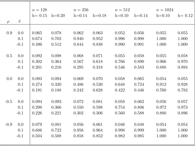
To investigate empirically the size and power behavior of the test T

, 500 repli- cations of the bivariate process (5.1) have been generated for different sample sizes n and different values of the dependence parameter ρ and the deviation parameter δ. The nonparametric estimators involved in our testing procedure have been calcu- lated using Parzen’s kernel (see Priestley (1981), p. 448) and different values of the smoothing bandwidth h. Furthermore, to obtain the critical points of the test using the bootstrap procedure proposed, 1000 bootstrap replications have been generated.

The results obtained for α = 0.05 are reported in Table 1.

Please insert Table 1 here

As Table 1 shows, although the test leads to some over rejection for the smallest sample size considered, the situation improves rapidly as the time series length n increases with the test achieving the desired size behavior. This behavior is not surprising since due to the allowed dependence between the individual time series, implementation of the test requires nonparametric, frequency domain estimation of the entire cross-correlation structure of the underlying m-dimensional process which is a difficult task. Concerning the power behavior of the test, we observe that the test leads to high rejection rates even for small differences between the two spectral densities, like those considered in the Monte Carlo experiment (δ = ±0.1).

Interestingly detecting differences between the spectral densities under independence (ρ = 0) appears to be more difficult that under dependence (ρ 6= 0). The explanation for this is given by formula (4.2) of the power function. Notice that for the particular bivariate process (5.1) considered, it is easily seen that κ

(λ) = ρ

for all λ ∈ [0, π], which by straightforward calculations yields

µ

= (1 − ρ

) 1

√ h Z

K

(x)dx, and τ

= (1 − ρ

)

1 π

Z ³ Z

K(x)K (x + y)dx

´

dy.

Now, other things being equal, if ρ

= κ

(·) = 0, i.e., if the two processes are in- dependent, then µ

and τ

achieve their maximal value leading to a large value of (µ

+ τ

z

)/(τ

√

Nh) and, consequently, to a drop of power. On the other hand as ρ

= κ

(·) increases, i.e. as the cross-correlation between the two processes becomes stronger, then µ

and τ

decrease, leading to a lower value of (µ

+ τ

z

)/(τ

√

Nh) and, therefore, to an increase of power.

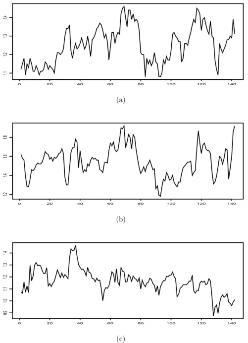
5.2. Analysis of grain price data. The data set considered consists of monthly

averages of grain prices for corn, wheat and rye in the United States of America for

the period January 1961 to October 1972. It has been discussed in Ahn and Reinsel (1988) and a complete description is given in Reinsel (2003). The original three- variate series is shown in Figure 1. We test the hypothesis that all three spectral densities are equal using the discretized statistic T

. For this Parzen’s smoothing kernel is used with a value h = 0.1 for the bandwidth obtained by means of a cross- validation criterion [Beltr˜ao and Bloomfield (1987)] applied to the pooled spectral density estimator w(λ). For this choice of the smoothing parameters the value of the b test statistic is equal to T

= 2.005, which compared with the upper 5% critical point 0.5057 obtained using B = 1000 bootstrap replications, leads to a rejection of the null hypothesis that the autocovariance structure of the three series is identical.

Figure 2a) shows on a log scale, the estimated individual spectral densities together with the estimated pooled spectral density w(λ). b

To get a deeper insight into the reasons leading to the above rejection of the hypothesis of equal spectral densities, and to investigate more closely were the differences between the individual spectral densities lie, we consider the statistic Q

(λ

) = ( f b

(λ

)/ w(λ b

) − 1)

calculated for λ

= 2πj/n, j = 0, 1, . . . , [n/2].

Notice that Q

(λ

) describes for every frequency λ

, the squared difference be- tween the estimated rth individual spectral density f b

(λ

) and the pooled spec- tral density w(λ b

) and that the test statistic T

can be approximately written as T

≈ 2πm

n

P

r=1

P

j=−ν

Q

(λ

), ν = [(n − 1)/2]. Large values of Q

pin- point, therefore, to frequencies where the spectral density of the rth series devi- ates from the pooled spectral density. A plot of the statistic Q

(λ

) for differ- ent frequencies and for each of the three price series considered is given in Figure 2b). To better evaluate the plots shown we include in the same figure an esti- mate of the upper 5%-percentage point of the distribution of the maximum statistic M

= max

max

Q

(λ

), under the hypothesis that all spectral densities are equal. To estimate the upper 5% percentage-point of this distribution we use the bootstrap procedure described in Section 3 to generate B = 1000 replications of M

= max

max

Q

(λ

), where Q

(λ

) = ( f b

(λ

)/ w b

(λ

) − 1)

and f b

(λ) and w b

(λ) are defined in Step 3 of the aforementioned bootstrap algorithm.

Please insert Figure 1 and Figure 2 about here

As Figure 2 shows, the autocovariance structure of corn and ray prices seem to

be very similar and different to that of wheat prices. The differences lie not only

in the fact that wheat prices have a larger variance compared to the other two

prices, but also that the spectral density of wheat prices show a moderate peak at

frequency λ = 0.796 which corresponds to a cyclical component of approximately 8

months and which is not apparent in corn and rye prices; cf. Figure 2b). It is worth

mentioning here, that these findings are in contrast to what could be expected by

a simple inspection of the time series plots of the three series shown in Figure 1.

Such an inspection suggests namely that corn and wheat prices behave similar and differently to ray prices.

6. Proofs Proof of Theorem 3.1: Note first that

N √ h m

X

r=1

Z ³ b f

(λ) b w(λ) −1

´

dλ = N √ h m

X

r=1

Z ³ b f

(λ) − w(λ) b w(λ)

´

dλ+O

(sup

λ

| w(λ)−w(λ)| b

´ ,

where the second term is o

(1) because max

sup

| f b

(λ) − f

(λ)| → 0, in probability, as n → ∞. Let

(6.1) T e

= N √

h m

X

r=1

Z

( f b

(λ) − w(λ)) b

1 w

(λ) dλ, and observe that

f b

(λ) − w(λ) = b 1 n

X

j

K

(λ − λ

)V

, where V

= X

s=1

g

I

(λ

) and g

= (δ

− m

). Verify by straightforward calculations that

(6.2) E[V

] = O(log(n)/n)

and that (6.3)

Cov(V

, V

) =

 

 P

s1=1

P

s2=1

g

g

|f

(λ

)|

+ O(n

) if j

= j

O(n

) if j

6= j

.

We then get E[ T e

] =

√ h n

X

r=1

Z X

j1

X

j2

K

(λ − λ

)K

(λ − λ

)dλ

× 1

w

(λ) Cov(V

, V

) + O( √

h log(n))

=

√ h n

X

r=1

Z X

j

K

(λ − λ

)Var(V

) 1

w

(λ) dλ + O( √

h) + O( √

h log(n))

= h

1 2π

Z

K

(x)dx X

r=1

X

s1=1

X

s2=1

g

g

Z

κ

(λ)dλ + o(1),