Scientific Computing I

Scientific Computing I

Wintersemester 2018/2019 Prof. Dr. Carsten Burstedde

Jose A. Fonseca

Exercise Sheet 3.

Exercise 1. (Maximum principle) (6 Points)

Let Ω a bounded domain inR^dand La second order linear elliptic differential operator and u∈ C²(Ω)∩ C( ¯Ω). Assume that

Lu=f ≤0 in Ω. (1)

Show that uattains its maximum on the boundary of Ω.

Hint:

• First prove the case f <0 assuming that there is an x0 ∈Ω with u(x0) = sup

Ω

u >sup

∂Ω

u. (2)

Perform a suitable coordinate transformation to obtain a contradiction.

• The casef ≤0 can be handled like the previous case by considering

w(x) =u(x) +δ||x−x₀||², (3) forx₀ as in (2) and someδ >0 sufficiently small.

Exercise 2. (Corollaries of the maximum principle) (6 Points) Let Ω a bounded domain inR^dand La second order linear elliptic differential operator.

a) Ifu, v∈ C²(Ω)∩ C( ¯Ω) satisfy

Lu≤Lv in Ω, (4)

u≤v on∂Ω, (5)

prove thatu≤v in Ω.

b) For the differential operator Lu:=

d

X

i,k=1

aik(x)uxixk +c(x)u, withc(x)≥0, (6) prove the following weaker form of the maximum principle: IfLu≤0, then

sup

x∈Ω

u(x)≤max{0, sup

x∈∂Ω

u(x)}. (7)

Hint: Lu−cu is elliptic.

1

-6 -3 0 3 6 0

3 6 9

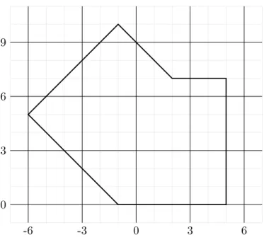
Figure 1: Grid and domain for Exercise 4.

Exercise 3. (6 Points)

Let Ω ⊂ R and u : Ω → R a sufficiently smooth function. For h₁, h₂ we consider T u: Ω→Rdefined as

T u:=αu(x−h₁) +βu(x) +γu(x+h₂). (8) Determine the coefficients α=α(h₁, h₂), β=β(h₁, h₂), γ =γ(h₁, h₂) such that

a) T u(x) approximatesu⁰(x) with order as high as possible.

b) T u(x) approximates u⁰⁰(x) with order as high as possible.

Hint: Determine the coefficients such that the formula is exact for polynomials with the degree as high as possible.

Exercise 4. (6 Points)

Let Ω be the domain depicted in Figure 4. Suppose we want to compute a finite difference approximation to the solution of Laplace’s equation ∆u = 0 with Dirichlet boundary conditions on Ω. To this end we employ a uniform mesh Ω_h with spacing h = 3, see Figure 4, and the five-point stencil approximation of the Laplace operator.

a) Give a suitable numbering for the points in Ω_h and ∂Ω_h. b) Write down the corresponding system of equations.

2