Incremental Clone Detection
Diploma Thesis
Submitted by
Nils G¨ ode
on
1
stSeptember 2008
University of Bremen
Faculty of Mathematics and Computer Science Software Engineering Group
Prof. Dr. Rainer Koschke
Acknowledgements
I would like to thank the members of the Software Engineering Group for discussing my ideas and giving me feedback. Special thanks go to Rainer
Koschke and Renate Klempien-Hinrichs for supervising this thesis.
Furthermore, I would like to apologize to my family and friends, who did not get the share of my time that they deserved.
Declaration of Authorship
I declare that I wrote this thesis without external help. I did not use any sources except those explicitly stated or referenced in the bibliography. All parts which have been literally or according to their meaning taken from publications are indicated as such.
Bremen, 1st September 2008
. . . . (Nils G¨ode)
Abstract
Finding, understanding and managing software clones — passages of dupli- cated source code — is of large interest, as research shows. However, most methods for detecting clones are limited to a single revision of a program.
To gain more insight into the impact of clones, their evolution has to be understood. Current investigations on the evolution of clones detect clones for different revisions separately and correlate them afterwards.
This thesis presents an incremental clone detection algorithm, which detects clones in multiple revisions of a program. It creates a mapping between clones of one revision to the next, supplying information about the addition, deletion or modification of clones. The algorithm uses token-based clone detection and requires less time than using an existing approach to detect clones in each revision separately. The implementation of the algorithm has been tested with large scale software systems.
Contents
1 Introduction 1
1.1 Software Clones . . . 1
1.2 Detecting Clones . . . 2
1.3 Research Questions . . . 5
1.4 Thesis Structure . . . 8
2 Background 9 2.1 Tokens and Token Tables . . . 9
2.2 Fragments and Clone Pairs . . . 10
2.3 Suffix Trees . . . 13
2.4 Clone Pairs and Suffix Trees . . . 17
2.5 Clone Detection Using clones . . . 19
3 Incremental Clone Detection 23 3.1 Multiple Token Tables . . . 23
3.2 Generalized Suffix Tree . . . 24
3.3 Integrating IDA. . . 31
3.4 Preparations . . . 32
3.5 Processing Changes . . . 33
3.6 Post Processing . . . 37
4 Tracing 41 4.1 Changing Clone Pairs . . . 43
4.2 Ambiguity of Changes . . . 45
4.3 Integration into IDA . . . 46
4.4 Matching Clone Pairs . . . 48
4.5 IDA in Pseudocode . . . 53
5 Evaluation 55 5.1 Test Candidates . . . 55
5.2 Testing Correctness . . . 60
5.3 Testing Performance . . . 63
5.4 Summary . . . 69
6 Conclusion 73 6.1 iClones and its Different Phases . . . 73
6.2 Summary of Results . . . 75
6.3 Future Research . . . 76
6.4 Applications forIDA . . . 78
A Supplying Data to iClones 81
B Extended Output Format 83
List of Figures 86
List of Tables 87
References 89
1 Introduction
To be faster or not to be faster:
That is the question!
1.1 Software Clones
Duplication of source code is a major problem in software development for different reasons. The source code becomes larger [MLM96] and more diffi- cult to understand, as copied passages have to be read and understood more than once [BYM+98]. A very serious issue arises from errors, bugs, found in any of the copies. In a lot of cases, copies are not created to be identical parts of code, but serve as basic structure for the new code to be written.
This means that slight changes are made to copies like renaming identifiers or changing constants [MLM96]. The more changes are made to the copies, the harder they become to trace. If bugs are found in the unchanged part, there are no sophisticated means of retrieving all other copies which need to be changed as well [Bak95, DRD99, Joh94, KKI02, Kon97]. This might lead to inconsistent changes of parts which are actually meant to be equal [KN05, Kri07].
Apart from the negative side, there is quite a diverse range of more or less comprehensible reasons for copying source code. The first striking reason is simplicity. It is often easier to copy and maybe slightly modify an existing portion of code than rethinking and writing things from scratch. This re- duces the probability of introducing new bugs, assuming the original code is known to work reliably [Bak95, BYM+98, DRD99, Joh94]. In highly op- timized systems, the overhead of additional procedure calls resulting from anextract method refactoring [Fow99] might not be acceptable. Parts of the code which are frequently executed are repeated instead of being abstracted into a new function [Bak95, BYM+98, DRD99, KKI02]. Architectural rea- sons, which include maintenance issues and coding style, might also require the repetition of code [Bak95, MLM96, BYM+98]. In addition to inten- tionally duplicated code, passages might be accidentally repeated. Uninten- tional repetition might emerge from frequently used patterns of the program- ming language or certain protocols for using libraries and data structures [BYM+98, KKI02]. Finally, non-technical issues can lead to code duplica- tion. If a programmer is assessed by the amount of code he or she writes, it is quite tempting to copy portions of code [Bak95, DRD99].
Although the negative impact of copied source code passages,clones, is not yet proven and several works discuss this topic contrarily [KG06, KSNM05,
Kri07, LWN07], information about the presence and evolution of clones is of great interest to study their influence on a system. Several approaches have been presented for finding and analyzing clones. The following section gives an overview over different methods used in software clone detection.
1.2 Detecting Clones
Preventing duplication of code right from the start is a rather illusive ob- jective as there are diverse reasons for copying passages of source code as mentioned above. Instead, a lot of effort is spent on finding clones in exist- ing source code using a clone detection algorithm. The termsoftware clone detection summarizes all methods that focus on finding similar passages of source code in a software system.
Different algorithms operate on different abstractions of a program to find clones. The most basic abstraction is the source code itself. Certain ap- proaches use the source text, with or without normalizing it, and find clones by applying textual comparison techniques [DRD99, Joh94, WM05]. With- out normalizing the source code, any yet so small difference like whitespace or comments in source passages can prevent tools from reporting clones.
Though textual comparison is relatively fast and easy to apply, the qual- ity of the results might lack from disregarding any syntactic or semantic information of the source code.
Other methods operate on the token string (see Section 2.1) that is produced from the program’s source code by running a lexer on it. By knowing some- thing about the syntax of the program, these methods are able to abstract from certain aspects of the source text like whitespace and text format- ting in general. Within the string of tokens, similar substrings are searched and reported as clones [Bak95, CDS04, KKI02, LLM06]. The advantage of token-based clone detection is that it performs very well, as the source code needs only to be converted into a string of tokens. The detection is also language independent as long as there exists a lexer for the language the source code is written in. Another benefit is that the source code does not need to be compilable and the detection can be run in any stage during the development of a program.
Yet other approaches search for clones based on theAST (Abstract Syntax Tree) of the program. Within the AST, subtrees are compared against each other and sufficiently similar subtrees are reported as clones. As the number of comparisons can rapidly grow fast due to an AST withnsubtrees requir- ingn2 comparisons, different criteria are used to select trees which need to be compared against each other [BYM+98, EFM07, JMSG07, Yan91]. Other
methods use the AST just as an intermediate result and do further process- ing in order to find clones [KFF06, WSvGF04]. As the syntactic structure of a program is represented inside the AST, tree-based approaches are able to report clones which are usually not detected by the previous methods.
These include for example commutative operations where the order of the two operands has been inverted. Although the usefulness of reported clones is increased, performance is a critical issue for tree-based detection.
Apart from the AST, thePDG (Program Dependency Graph)might be con- sidered for drawing conclusions about clones [KH01, Kri01]. A PDG rep- resents the data flow and control flow inside a program. Inside the PDG, similar subgraph structures are used to identify clones. The additional in- formation that is obtained from the PDG allows to improve the quality of reported clones. On the other hand, creating a PDG and searching clones within it can be very costly. Like tree-based detection, graph-based ap- proaches depend on the programming language of the program analyzed.
A rather different approach to finding clones is based on metrics retrieved for syntactic units of the program [DBF+95, MLM96, PMDL99]. If certain units are equal or similar in their metric values, they are supposed to be clones. This is based on the assumption, that if two units are equal in their metric values, they are equal — or at least sufficiently similar — to be reported as clones. In any case, metrics have to be chosen carefully in order to retrieve useful results.
All these approaches have advantages and drawbacks. Which method yields the best results for a given scenario depends to a large extend on the spe- cific application. A comparison of selected clone detection methods which operate on different abstractions of a program can be found in [Bel07].
Though being quite diverse, all these approaches have in common that they are all targeted at analyzing a single revision1 of a program. For many applications this is the desired behavior, but still there are scenarios which require more than the analysis of a single revision. Considering all questions aimed at the evolution of software clones requires analyzing more than one revision of a program. Current approaches trying to answer evolutionary questions about software clones usually start by analyzing each revision of the program separately, utilizing one of the existing detection techniques.
After the clones have been identified for each revision, clones of different re- visions are matched against each other based on some definition of similarity [ACPM01, KSNM05, Kri07]. If a clone in revisioniis adequately similar to a clone in revisioni−1, it is assumed that the clone is the same. Some of
1Within the context of this thesis, arevisionis seen as a state of program’s source code at a specific point of time
these methods are summarized in Section 4. There are however two major issues concerning these approaches.
• Although running adequately fast, all clone detection algorithms still need a noticeable amount of time to produce their results. If a huge amount of revisions of a program is to be analyzed, the time tall re- quired to get results, is a multiple of the time needed to process a single revisiontsingle. Assuming that the timetsingle is approximately the same for every revision, the overall time to analyzenrevisions is
tall ≈n·tsingle
The assumption is, that a lot of processing steps are repeated redun- dantly. Intermediate results which might be reused in the analysis of the next revision are discarded and need to be recomputed for every revision, causing an unnecessary overhead. This results in large parts of the program to be analyzed over and over again for each revision, although most parts of the source code did not change at all.
• If every revision of the software is analyzed on its own, the results are independent sets of clones. An important thing missing is the mapping from the clones of one revision to the clones of the next revision. The information about the changes that happened to each single clone is not provided and has to be calculated later.
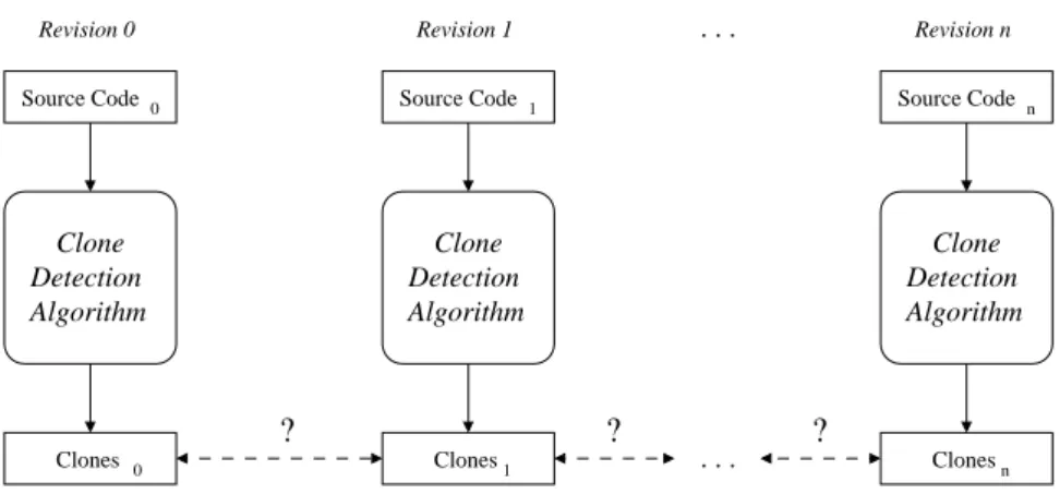
Figure 1 shows conventional clone detection applied to multiple revisions of a program. Assuming that changes between revisions i and i+ 1 stay in a limited range, many calculations are done redundantly. Furthermore, the mapping between clones of revision i and i+ 1 is not created by the algorithm as every revision is analyzed on its own.
The issues mentioned above and the fact that more and more questions are directed towards the evolution of clones [HK08] suggest a detection algo- rithm that is designed to analyze more than one revision of a program and tries to exploit this attitude as much as possible. Having such an algorithm is desirable as it would most likely save huge amounts of time when analyzing many revisions of a program. Furthermore, it would make clones traceable across revisions and allow analyses of the evolution of clones. This in turn would help answering the question of the harmfulness of clones. The answer is important, because if clones are not to be considered harmful, then the effort spent on finding and removing them is not legitimate.
Source Code1
Source Code0 Source Coden
Detection Algorithm Clone
Detection Algorithm Clone
Detection Algorithm Clone
Revision 0 Revision 1 . . . Revision n
? ? ?
. . .
Clones 0 Clones1 Clonesn
Figure 1 – Conventional clone detection applied to multiple re- visions of a program. Calculations are unnecessarily repeated and the mapping between clones is unsure. Solid arrows indicate input and output of the algorithm. Dashed arrows represent the mapping between two clone sets.
Another scenario that might be thought of, is the integration of “on-line”
clone detection into an IDE (Integrated Development Environment). On- line clone detection reports any changes of clone pairs to the user while he or she is editing the source files of a program. This prevents the user from accidentally introducing new clones or doing inconsistent changes to existing clones. The detection algorithm runs in the background and when the user changes a file, the set of clones is updated accordingly and changes to clones are reported to the user.
1.3 Research Questions
The overall task of this thesis is to develop and implement an incremen- tal clone detection algorithm that requires less time for clone detection in multiple revisions of a program than the separate application of an existing approach. In addition, a mapping between the clones of every two consecu- tive revisions must be generated. To guide the development and assist the achievement of the task, a number of research questions are given which are to be answered within this thesis.
1.3.1 Multi-Revision Detection
The first part of the task addresses the timetall which is needed to analyze n revisions of a program’s source code. The assumption is, that time can
be saved by eliminating unnecessary calculations resulting from discarding intermediate results. It is desirable to maketall < n·tsingle true. Instead of starting from the very beginning, the analysis of a revision should reuse and modify results of the previous revision. This requires an overview over all re- sults which are produced during the clone detection process and assessment of whether they might serve for being reused.
Question 1 – Which intermediate results can potentially be reused to ac- celerate multi-revision clone detection?
It is very unlikely, that reuse can happen straight away, because the inter- mediate results are not designed for being reused. It is very probable that certain problems arise which must be solved to make the results reusable.
Question 2 –Which problems arise from reusing intermediate results and how can they be solved?
After solutions have been given to the problem of reusing intermediate re- sults, a concrete algorithm needs to be presented that puts multi-revision clone detection into practice. The algorithm has to implement the conclu- sions drawn from answering the previous two questions.
Question 3 –How does an incremental clone detection algorithm look like?
1.3.2 Tracing
Apart from improving the performance, clones of one revision are to be mapped to the clones of the previous revision. In the simplest case, clones remain untouched and no change happens to any clone. On the other hand, clones can be introduced, modified, or vanish due to the modification of the files they are contained in. The different changes that can happen to a clone must be summarized.
Question 4 –Which changes can happen to a clone between two revisions?
Knowing about the nature of changes, it might be possible to draw conclu- sions about changed clones from the modification of intermediate results. It is assumed that changes can be derived and do not need to be recreated in a separate phase.
Question 5 –How can changes to clones be derived while reusing interme- diate results?
If not all changes can be concluded from the modification of results, the remaining changes have to be obtained in a post-processing step. This re- quires a method that is able to locate a clone from revision i in revision i+ 1.
Question 6 – How can a clone in revisioni be found in revision i+ 1?
1.3.3 Implementation and Evaluation
It is not only required to present the conceptual ideas for incremental clone detection, but also to implement them. The underlying use case for the implementation of an incremental clone detection algorithm is, that given multiple revisions of a program, the clones in each revision are to be detected.
It is required, that the incremental algorithm produces its results faster than separate applications of an existing approach. As implementing clone detection from scratch goes far beyond the scope of this thesis, an existing implementation is to be modified. This limits the diversity of theoretical and practical options that can be explored.
The existing tool which serves as a starting point for the implementation is the toolclones from the projectBauhaus2. The performance of the new algorithm’s implementation is tested against the performance of clones to keep results comparable.
Question 7 –How does the new implementation perform in comparison to clones, regarding time and memory consumption?
It is assumed, that no general statement can be made about how much time can be saved by using incremental clone detection. The time most likely depends on different factors which influence the detection process.
Question 8 –Which factors influence the time required by the new imple- mentation?
The answers to these questions are gained by developing and implementing the incremental clone detection algorithm. They are given at the respective locations within this thesis.
2http://www.bauhaus-stuttgart.de/
1.4 Thesis Structure
This thesis is organized as follows. Section 2 introduces the necessary con- cepts related to software clone detection. It explains the clone detection process as implemented in the toolclones. Section 3 answers the questions related to multi-revision analyses and presents an incremental clone detec- tion algorithm. Section 4 explains changes that can happen to clones and describes how clones can be traced across revisions. Section 5 summarizes the tests that have been run to answer the questions directed at the perfor- mance of the implementation. Conclusions and ideas for future development are given in Section 6.
2 Background
This section introduces the necessary concepts for understanding the prob- lem of incremental clone detection and the solution presented in this thesis.
Section 2.1 explains tokens and token tables. Section 2.2 explains terms re- lated to software clone detection which are unfortunately used with different meanings by different publications. Therefore it is necessary to have a com- mon understanding of these terms in order to avoid any confusion. Section 2.3 introduces the concept of suffix trees. The relation between clone pairs and suffix trees is outlined in Section 2.4. Finally, Section 2.5 introduces token-based clone detection as implemented in the toolclones by describing the major phases.
2.1 Tokens and Token Tables
Throughout this thesis, the word token will be used frequently as clone detection using the tool clones is based on sequences of tokens forming clones. Aho et al. define a token as follows:
“[. . . ] tokens, that are sequences of characters having a collective meaning.” [ASU86]
A token is an atomic syntactic element of a programming language (i.e. a keyword, an operator, an identifier,. . . ). In addition, clones also recognizes preprocessor directives as tokens. A sequence of successive tokens is referred to as a token string. Each token has certain properties which are accessed in different stages of the clone detection procedure. Among the important properties of a token are the following:
• Index: The index of the token inside the token table in which it is contained.
• Type: Every token has a type describing the nature of the token.
Example types are+,=,while or<identifier>.
• Value: Tokens which are identifiers or literals have a value in addition to their type. Identifiers have their actual name being the token’s value. Literals have the value represented by their string, for instance, literal “1” has an integer value 1.
• File: The source file which contains the token.
• Line: The line in the source file in which contains the token.
• Column: The column in the source file in which the token starts.
Lines and columns are counted starting from 1.
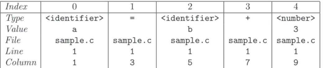
Tokens are stored inside atoken table which holds a number of tokens along with their properties. By using a token’s index, the token table allows fast access to the token’s properties. A token table is created using ascanner or lexer which translates a source code file into a sequence of tokens. A simple token table is shown in Table 1.
Index 0 1 2 3 4
Type <identifier> = <identifier> + <number>
Value a b 3
File sample.c sample.c sample.c sample.c sample.c
Line 1 1 1 1 1
Column 1 3 5 7 9
Table 1– A sample token table for the inputa = b + 3contained in a file calledsample.c.
2.2 Fragments and Clone Pairs
When talking about software clones, it is very helpful to have a shared under- standing of terms and concepts used to describe clones and relations among them. Far too often, terms likecloneand clone pair are used inconsistently, leading to confusion or requiring additional explanation whenever used.
Although the word clone is used in almost every publication related to software clone detection, there exists no definition and no sufficiently com- mon understanding of what is to be treated as a clone and what is not [KAG+07, Wal07]. To avoid any misunderstanding, this thesis will not give any concrete meaning to the word clone on its own. Different words are used to describe related concepts. The following sections explain the terms fragment andclone pair and state how they are used within this document.
2.2.1 Fragment
Throughout this thesis, the wordfragment refers to a passage in the source code. A fragment consists of a sequence of consecutive tokens. Having a well-defined location, a fragment can be described as a triple
f ragment= (f ile, start, end)
withfile being the file in which the fragment appears,start the first token3 in the given file which is part of the fragment, andend representing the last token belonging to the fragment. All tokens betweenstart andend are part of the fragment.
A fragment on its own is not very helpful without knowing whether and which parts of the source code it actually equals. The relation between fragments is described in form of aclone pair.
2.2.2 Clone Pair
A clone pair is the relation between exactly two fragments that are similar to a certain degree or even identical. A clone pair can be described as
clone pair = (f ragmentA, f ragmentB, type)
where f ragmentA and f ragmentB are fragments as described above. In order to express different levels of similarity between two fragments, the clone pair has atype in addition to the two source code fragments. Among various descriptions of the similarity between code fragments is the one classifying clone pairs according to four different types. Type 1 to type 3 describe a textual similarity between fragments whereas type 4 refers to fragments which are similar in their semantic.
Type 1: Within a clone pair of type 1, both fragments are exactly equal disregarding comments and whitespace. All tokens at corresponding posi- tions in the two fragments are identical in their type and their value. An example of a type-1 clone pair can be found in Figure 2.
1 int a = 0;
2 b = a * a ;
3 string = " Peter ";
(a)f ragmentA
1 int a = 0;
2 b = a * a ; // Comment 3 string = " Peter ";
(b)f ragmentB
Figure 2– A clone pair of type 1.
3For further processing of fragments — especially by humans — it might be more helpful to give the start and end of a fragment in line numbers. Therefore the token information is converted to line information just before outputting the result.
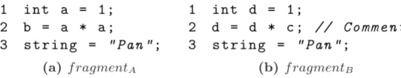
Type 2: A clone pair of type 2 consists of two fragments whose tokens are identical in their type. In contrast to a type-1 clone pair, the values of identifiers or literals do not need to be identical. Type-2 clone pairs are those where source code has been copied and the names of identifiers have been changed afterwards. Depending on the application, it is sometimes required, that identifiers have been consistently changed, meaning there needs to exist a one-to-one mapping between the identifiers of the first fragment to the ones of the second fragment. Baker presented a method for finding type-2 clone pairs with consistent changes, also referred to as parameterized duplication [Bak97]. An example clone pair of type 2 is shown in Figure 3.
1 int a = 1;
2 b = a * a ; 3 string = " Pan ";
(a)f ragmentA
1 int d = 1;
2 d = d * c ; // Comment 3 string = " Pan ";
(b) f ragmentB
Figure 3– A clone pair of type 2 with inconsistent renaming.
In addition to type-1 and type-2 clone pairs, there are two more types which describe more inconspicuous relations between clones. These are given for completeness, but are not considered in this thesis due to their complexity and lack of a concise definition.
Type 3: Type-3 clone pairs combine two or more adjacent clone pairs of the preceding types. These clone pairs may be separated by small code fragments which are not identical. The motivation for type-3 clone pairs is to find pairs which have been modified by inserting or removing tokens from one of the fragments. Such a situation may indicate that a mistake has been found and corrected in one of the fragments, but the other fragment stayed unchanged.
Type 4: Between the fragments of a type-4 clone pair exists an even more vague relation concerning the behavior of the fragments. Code fragments belonging to a clone pair of type 4 carry out similar tasks and are similar in their semantic.
An important property of clone pairs is, that the relation between the two fragments is symmetric, meaning that the existence of clone pair cp1 = (f ragmentA, f ragmentB, type) requires the existence of clone pair cp2 = (f ragmentB, f ragmentA, type). Though being formally correct, the infor- mation contained in both clone pairs is the same and therefore this docu- ment abstracts from the order in which the two fragments appear, making the following always true.
(f ragmentA, f ragmentB, type) =cp= (f ragmentB, f ragmentA, type) To ease the processing of clone pairs, each pair isnormalized upon creation.
In a normalized clone pair, it is fixed which fragment is f ragmentA and which isf ragmentB.
For clone pairs with type ≤ 2, the relation between the two fragments is not only symmetric, but also transitive. From the existence of pairscp1 = (f ragmentA, f ragmentB, type) and cp2 = (f ragmentB, f ragmentC, type) follows, that the paircp3= (f ragmentA, f ragmentC, type) must exist.
The algorithm described in this thesis relates similar code fragments in terms of clone pairs analogously to the tool clones. Still, other relations between code fragments exist. Among them is the relation which groups two or more similar fragments. This relation is usually called clone class or clone community [MLM96].
2.3 Suffix Trees
Incremental clone detection, as described in this thesis, is based on gen- eralized suffix trees. Therefore it is essential to have an understanding of what suffix trees are and how they represent suffixes of strings of tokens.
Many different notions for strings, substrings and suffix trees have been given [Bak93, FGM97, McC76]. This thesis follows the notion presented in [FGM97] in most parts. Although the concepts of strings and suffix trees are described by using strings of characters, the same applies to strings of tokens.
2.3.1 Notion of Strings
A stringXwhich is of lengthmis represented asX[0, m−1]. The character at position i in X is denoted as X[i]. Any substring of X, containing the characters at positionsi, i+ 1, . . . , jis written asX[i, j] with 0≤i≤j < m.
It follows that every substring X[j, m−1] is a suffix and every substring X[0, i] is a prefix of X. The string X contains m prefixes and m suffixes.
To ensure, that no suffix is a prefix of any other suffix, the last character at position m−1 of the string is globally unique. It does not match any other character from stringX and no character from any other string. The unique character is represented as $, respectively $1, $2, . . . , $nif more than one string is used.
2.3.2 Nodes and Edges
A suffix tree is a tree-like data structure which represents all suffixes of a given string X. Disregarding suffix links, which are introduced in Section 2.3.3, the suffix tree is a tree. Every leaf of the suffix tree represents one suffix ofX. This makes the suffix tree very useful for solving many problems that deal with strings. Among the many applications, McCreight was one of the first to create a suffix tree based upon which equal substrings within a string can be searched [McC76].
Every edge of the suffix tree is labeled with a substring ofX. To significantly reduce the space needed by the tree, it is essential to specify the substring by the indices of its first and last characteriandj instead of specifying the complete substring. This way, every edge label is a tuple (i, j) referring to the substringX[i, j].
Every edge is connected to two nodes, thestart nodebeing the node directed towards the root and the other one being its end node. An edge is called internal if its end node is the start node of at least two other edges. If the end node is not the start node of any other edge, then the edge is called external. Note, that it is not possible for any node to have just one edge of which it is the start node. The exception to this rule is the root node of the tree in case ofX being the empty string $.
Two edges are calledsiblings if they have the same start node. An important property of suffix trees is, that no two siblings labels start with the same character.
Every node except the root has a parent edge, being the edge of which it is the end node. In addition, every node except the root has aparent node being the start node of its parent edge. For the root of the tree, parent edge and parent node are undefined. The path of a node is the string obtained by concatenating all substrings, referred to by the edge labels from the root to that node. Each node has apath length, which is length of its path. The path length for the root is 0.
Like edges, a node is calledinternalif it is the start node of at least two edges, otherwise it is calledexternal orleaf. Note that every external edge has an external end node and every external end node has an external parent edge.
Likewise, every internal edge has an internal end node and every internal node has an internal parent edge. Every external node represents a suffix of the stringX which is equal to the path of that node. Therefore, a suffix tree for a string of length m must have m external nodes and m external edges.
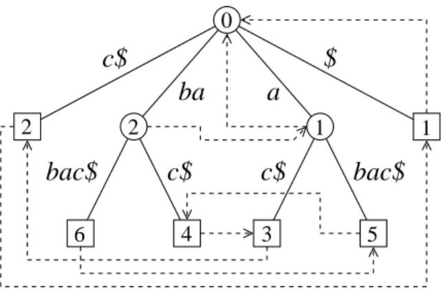
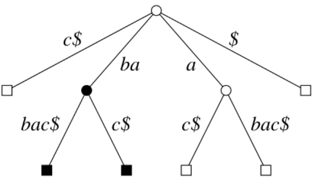
A suffix tree for the string X =babac$ is shown in Figure 4. Throughout this document, certain things are to be considered for the visualization of suffix trees. Squares represent external nodes, circles internal nodes. Solid lines are edges connecting the nodes. Though being expressed by start and end index, labels are usually shown as readable substrings to make the understanding of figures easier. Any exceptions to these conventions are mentioned in the description of the respective figure.
a
c$
2 2
0
1 1
5 3
4 6
bac$
c$
bac$
ba
$ c$
(a)Suffix tree with text labels.
2 2
0
1 1
5 3
4 6
(4,5)
(5,5)
(2,5) (4,5)
(2,5) (4,5)
(0,1) (1,1)
(b) Suffix tree with indices for labels.
Figure 4– Suffix tree for the stringX =babac$. The path length of every node is noted inside the node.
2.3.3 Suffix Links
In order to allow faster construction, suffix trees are augmented with so- called suffix links between nodes. If the path from the root to a node rep- resents the substringX[i, j], then the suffix link of that node points to the node whose path represents the substringX[i+ 1, j]. The suffix link of the root is undefined.
Suffix links do not only help in construction, but also allow for fast nav- igation inside a suffix tree. Following suffix links helps iterating over all suffixes of a given string from longest to shortest, because every suffix link points to the node whose path represents the next smaller suffix. As suffix links decrease the readability of suffix trees, they will usually not be drawn in figures within this thesis. The suffix tree from Figure 4 augmented with suffix links is shown in Figure 5.
2.3.4 Construction
For long strings and real applications, a fast construction algorithm for suffix trees is needed. Several construction algorithms that require time linear to
a
c$
2 2
0
1 1
5 3
4 6
bac$
c$
bac$
ba
$ c$
Figure 5– Suffix tree for the stringX =babac$ augmented with suffix links (dashed arrows).
the length of the input string have been presented [Bak97, McC76, Ukk95].
The two algorithms which are implemented and used by the toolclones are the following:
Ukkonen: Ukkonen presented an on-line algorithm for constructing suffix trees [Ukk95]. On-line refers to the algorithms property of processing char- acters or tokens of the input string from the beginning to the end. At any point of the construction, the suffix tree for the part of the string that has already been processed is available. There is no need to know the complete string upon starting the construction.
Baker (Parameterized Strings): Baker introduced an algorithm to find parameterized duplication in strings [Bak97]. In addition, she presents a modified version of McCreight’s algorithm, that allows construction of pa- rameterized suffix trees for parameterized strings. A parameterized string abstracts from the actual names of identifiers, but still preserves the order- ing among them. This constructor is used byclones if type-2 clone pairs are required to have a consistent renaming of identifiers.
2.3.5 Applications
The representation of all suffixes of a string in form of a suffix tree allows to run many different algorithms that solve common search problems in strings in adequate time [McC76]. Some example questions that can easily be answered with the suffix tree built for the stringX are:
• Is stringW a substring of X?
• Find all occurrences of a substring S inX.
• Find all maximal matches of substrings inX.
The last question is the one that is relevant for finding clones in software.
Assuming the whole source code is parsed into one token string, the search for maximal matches of substrings reveals code fragments that are equal and have therefore most probably been copied.
2.4 Clone Pairs and Suffix Trees
This section describes the relation between suffix trees and clone pairs. This relation is used byBaker’s algorithm for extracting maximal matches from a suffix tree and becomes relevant when the structure of the suffix tree is to be modified.
Each internal node of a suffix tree represents a sequence of characters or tokens that appears more than once inside the string from which the suffix tree was built. As the sequence has at least one identical copy, it is a clone.
The token sequence of the clone is identical to the path of the internal node.
How often the sequence appears in the string is determined by the number of leaves that can be reached from the internal node, because every leaf represents a different suffix of the string.
Among these clones, every pair that can be formed is a clone pair as defined in Section 2.2. However, many of these pairs are less interesting, because they are not maximal and covered by other pairs. According toBaker,
“A match is maximal if it is neither left-extensible nor right- extensible [. . . ]” [Bak93].
A clone pair cp= ((f ile1, start1, end1),(f ile2, start2, end2), type) is said to beright-extensible if the token inf ile1at positionend1+ 1 equals the token inf ile2 at positionend2+ 1. If that is the case, the match is not maximal, because both fragments can be expanded by one token to the right. If eitherend1 orend2 is the last token of the respective file, the match is not right-extensible, because at least one token is undefined.
A clone pair cp= ((f ile1, start1, end1),(f ile2, start2, end2), type) is said to beleft-extensible if the token inf ile1 at positionstart1−1 equals the token in f ile2 at position start2−1. This is also not recognized as a maximal
match. Analogous to right-extensibility, ifstart1 orstart2 denotes the first token of the respective file, the clone pair is not said to be left-extensible.
There is however one problem concerning this definition. It does not con- sider the case where one fragment is left-extensible and the other fragment is right-extensible and both fragments still contain the same sequence of tokens. Such situations appear in conjunction with self-similar fragments.
This results in clone pairs being reported as maximal although both frag- ments are extensible. Because there is no satisfactory solution to this prob- lem yet, this thesis will use the definition as it has been presented.
Concerning the extraction of clone pairs from the suffix tree, right-extensi- bility does not need to be explicitly checked if only fragments are combined that stem from leaves which are reached by different edges from an internal node. According to the definition of suffix trees, no pair of outgoing edges from that node can share the first character (or token) of their label. As this token is the first to the right and different for both fragments, the clone pair cannot be right-extensible. If however clone pairs were formed by leaves being reached from the same outgoing edge, the respective fragments must by definition be right-extensible. At least by the tokens of the outgoing edge which they share.
Left-extensibility can unfortunately not directly be read from the suffix tree and must be tested upon combining two fragments. If the resulting clone pair is left-extensible it is discarded, otherwise it is reported as being maximal.
Having found two leaf nodes n1 and n2 that share a sequence of tokens which is neither left-extensible nor right-extensible, a clone pair can be built as follows. The value of f ile1 equals the file information contained in the label of the parent edge ofn1. The indices start1 andend1 can be obtained by considering the indices of n1’s parent edge and the path length of node n1. The same applies to the second fragment using the noden2. The clone pair’s type is determined later in a post processing step. Important is, that all values can be determined in constant time.
Summing up, fragments relate to leaf nodes and clone pairs to internal nodes of the suffix tree. Indices for these can be calculated in constant time. Figure 6 shows a maximal match in a sample suffix tree.
a
c$ c$ bac$
bac$
ba
$ c$
Figure 6– Maximal match in the suffix tree for the stringbabac$.
The black external nodes represent the fragments of the clone pair.
The path from the root to the black internal node shows the cloned sequence of characters beingba. Note, that the path with label a of the second internal node is not a maximal match, becauseais left-extensible.
2.5 Clone Detection Using clones
Different approaches to clone detection have been briefly outlined in Sec- tion 1.2. This section explains the process of token-based clone detection as implemented in the tool clones from the project Bauhaus. Due to the underlying task of this thesis, the usage of clones and the adaptation of clones mechanisms to multi-revision clone detection is compulsory.
The toolclones runs five major phases to detect clones in a given program.
First, all source files are parsed into one large token string, then the suffix tree is built for that string. Within the suffix tree,Baker’salgorithm [Bak97]
is used for finding maximal matches which are filtered afterwards in order to discard uninteresting clone pairs. The last step consists of outputting the resulting set of clone pairs in the desired format.
2.5.1 Tokenizing
This is the first step in token-based clone detection and common to every compiler and every program that analyzes source code. All files that belong to the system in which clones are to be searched are collected and scanned by a lexer into a string of tokens. The token strings of all files are concatenated together to form a single string. This allows building a single suffix tree which contains the information about all suffixes of all files. If a single suffix tree was used for each file, no clone pairs could be found where the fragments stem from different files. A single tree for all files ensures that clone pairs can be found across files. Before concatenation, a unique file terminator token
is appended to the token string of each file. This ensures, that no fragments that cross file boundaries are part of clone pairs. The concatenated string is saved in a single token table that maps an index to information about the token at that position.
2.5.2 Suffix Tree Construction
After creating the token string of all tokens from the source code, the suffix tree for this string is built. Depending on the application, two construction methods for the suffix tree are available. The first construction algorithm is an implementation ofUkkonen’s algorithm [Ukk95], which directly builds the suffix tree for the token string. Although the algorithm has the benefit of being on-line, this is not important forclones, because the complete string for which the suffix tree is built is available before starting the suffix tree construction.
Another suffix tree constructor is available which implements the algorithm presented by Baker [Bak97]. The token string is first converted into a pa- rameterized token string. Based on the parameterized token string, the constructor builds a parameterized suffix tree. This constructor is used whenever parameterized clone detection is requested, because theUkkonen constructor is not able to build a parameterized suffix tree.
2.5.3 Extraction of Longest Matches (Baker)
In the third step, Baker’s algorithm pdup [Bak97] for extracting longest matches from the suffix tree is used to find potential clone pairs. To reduce the number of clone pairs that need to be processed in the following phases, some potential clone pairs can already be discarded. The most important criteria for discarding clones is the minimum length they need to have. The algorithm is already aware of this criteria and drops clone pairs which are not long enough to be reported. The result is a list of clone pairs, that all conform to the minimum length.
2.5.4 Filtering
Though a lot of clone pairs have already been dropped during the extraction of longest matches, the list of pairs most probably contains a lot of pairs that are of no interest (i.e. overlapping pairs or pairs which span more than
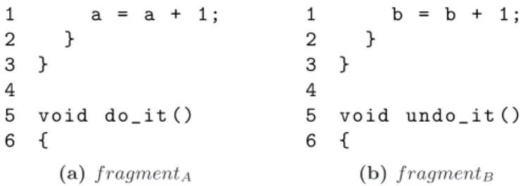
one syntactic unit as shown in Figure 7). To improve the result, several filtering phases are run.
The first phase determines the type of each clone pair. Due to the nature of pdup, only type-1 and type-2 clone pairs are extracted from the suffix tree.
For each clone pair, the fragment’s identifier tokens are checked for equality.
If a discrepancy is found, the pair is of type 2, otherwise of type 1.
Other filters include cutting clone pairs down to syntactic units, merging type-1 or type-2 clone pairs into type-3 pairs or removing overlapping clone pairs. Depending on the filters that are applied, this step is quite time intensive. It is not unusual, that a filter has a worst-case quadratic time complexity as every clone pair needs to be compared to every other clone pair.
2.5.5 Output
The last step consists of formatting the clone pairs and outputting them in the desired format. The information about the location of fragments needs to be converted from token indices into lines, to make the result readable for the user. Depending on the required format, each clone pair is emitted with the location of the two fragments and its type as well as its length.
1 a = a + 1;
2 }
3 } 4
5 void do_it () 6 {
(a) f ragmentA
1 b = b + 1;
2 }
3 } 4
5 void undo_it () 6 {
(b) f ragmentB
Figure 7 – A clone pair that is not very helpful as the token sequence of the fragments spans more than one syntactic unit.
3 Incremental Clone Detection
This section describes the Incremental Detection Algorithm IDA and con- cepts relevant to it. The motivation for IDA is to have an algorithm that analyzes multiple revisions of a program faster than the separate applica- tion of the tool clones on each revision. The motivation is based on the assumption that only a comparatively small amount of files change per re- vision, causing a lot of work to be done redundantly when rerunning every part ofclones. Therefore, internal results are not discarded, but reused and modified according to the files that changed for the respective revision.
The information which files have changed between any two consecutive re- visions is given to IDA together with the source code of each revision that is to be analyzed. IDA itself runs several phases for every revision, which consist ofpreparations,processing changes and a post processing stage.
To accelerate the detection of multiple revisions, the analysis of revisioni
must consider and reuse intermediate results ofrevisioni−1 as much as pos- sible. The intermediate results which can be reused are the data that are created during the clone detection process. A lot of this data are not directly part of the token-based clone detection process. Though being also reused as far as possible, they are not mentioned here due to their technical nature.
Answering Question 1, the data structures that are important for the clone detection process and which can potentially be reused are the token table, the suffix tree and the set of clone pairs. The time needed to create these takes a considerable amount of time of the whole detection process. For this reason, they are not discarded after the analysis of a revision, but kept in memory and reused for the next revision. However, some effort must be spent to make these data structures suitable for multi-revision detection.
Sections 3.1 and 3.2 answer Question 2 by explaining in which wayclones’
data structures must be modified in order to be reused. Section 3.3 shows how the incremental algorithm integrates into the analysis of multiple revi- sions. Sections 3.4 to 3.6 explain the different phases of whichIDAconsists.
3.1 Multiple Token Tables
The first data structure which is to be reused is the token table. As files are added and deleted from revision to revision, old tokens that are not needed anymore can be discarded and new tokens have to be read for new files. If
a single table is used, problems arise when files change and the token tables for the respective files need to be updated to conform to the new versions.
Assuming a file is deleted, its tokens have to be removed at some point from the token table, because otherwise the algorithm will sooner or later run into memory shortage. Recalling that the edges of the suffix tree are labeled by the start and end index of a substring, one has to ensure, that no label of the suffix tree references the part of the token table where tokens were discarded. This would require checking the complete suffix tree for dangling indices upon deleting a file. Even more critical, new indices that denote the same substring have to be found for every edge with invalid indices.
Apart from invalid indices, there is the problem of growing holes inside the token table, caused by files that have been deleted. One could try to fit new files into these spaces and fill the holes, but whatever token table man- agement is used, the management overhead will most likely be intolerable.
More complex methods, that remap indices to valid locations upon request- ing a token are of no use, because accessing a token from the token table is the most common action in the implementation and should therefore be as fast as possible. Any yet so small delay in accessing a token will add up to a significant amount.
These issues are the reason for IDA to not hold a single token table, but rather have one token table for every file. When a file is deleted, the token table for the respective file can just be dropped after the suffix tree has been updated. When a file is added, a new token table is created. The location of a token must therefore be extended to a tuple (f ile, index) instead of just having a single index. file selects the token table for the file in which the token is contained, and index denotes the position of the token inside that file. Section 3.2.2 describes how dangling references caused by the deletion of files are avoided.
3.2 Generalized Suffix Tree
In addition to changing the token tables when files have changed, suffixes of these files also have to be added and deleted from the suffix tree. This causes the structure of the tree to change in order to conform to the new token sequences of the changed files. Assuming concatenated token strings and a suffix tree for the complete string as practiced inclones, every external edge’s label spans all tokens to the very end of the token string including the tokens of all files following the edge’s file. If the token string becomes shorter (or longer), the label’s end index of every external edge would need to be changed. Many parts of the suffix tree have to be modified that are in
no way related to the file which has changed. It is desirable to only modify the edges related to the changed file and leave all other edges untouched.
To solve this problem,IDAuses ageneralized suffix tree[GLS92] that repre- sents suffixes of multiple strings instead of just a single string. The advan- tage of a generalized suffix tree is, that algorithms exist to efficiently insert or remove a string from the underlying set of strings and update the tree accordingly by only modifying the edges relevant for the respective file.
A generalized suffix tree represents all suffixes of all strings in a set of strings
∆ ={X1, X2, . . . , Xn}. It can be seen as the superimposition of the indi- vidual suffix trees of the strings in ∆. Whenever parts of edge labels are equal, they can be unified into a single edge, now serving for two or more strings from ∆. However, the tuples that label the edges must be expanded, because more than one string contributes to labeling the edges. The tuple (i, j) which referred to start and end position inside the string is extended to a triple also giving information to which string the indicesi and j refer.
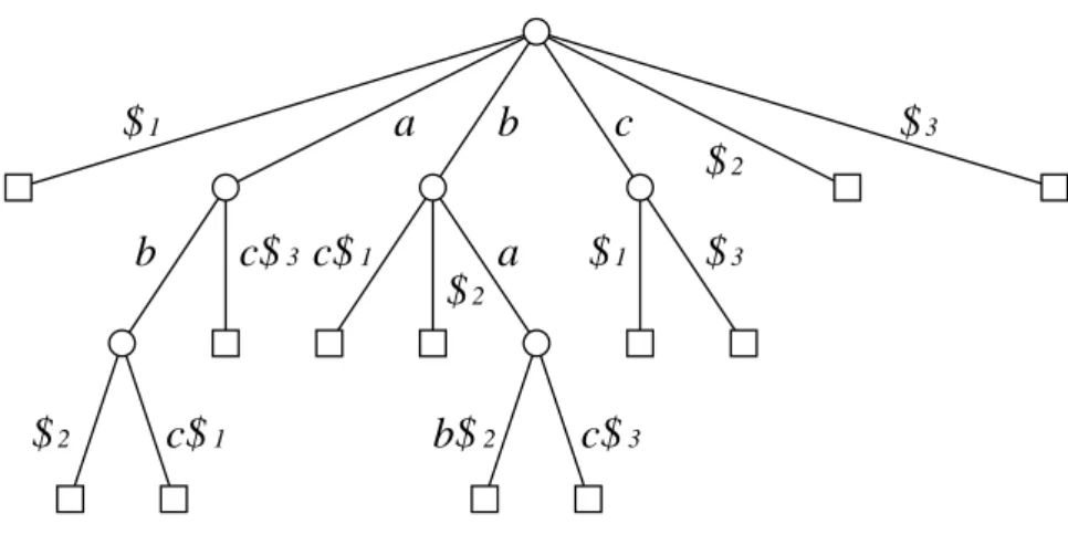
An edge label is now a triple (X, i, j), where i and j denote the start and end position of a substring inX. A sample generalized suffix tree for the set of strings ∆ ={abc$1, bab$2, bac$3} is given in Figure 8. It should be kept in mind, that every string Xi in ∆ has a unique endmarker $i, which does not match any other character or endmarker.
b$
2c$
3c$
1c$
1c$
3$
1$
3$
2$
1$
3$
2$
2c b
a
a b
Figure 8 – Generalized suffix tree for the set of strings ∆ = {abc$1, bab$2, bac$3}.
It is worth noting, that the generalized suffix tree for ∆ ={X1, X2, . . . , Xn} is isomorphic to the suffix tree which can be constructed from the concate- nated stringX1X2. . . Xn.
Furthermore an important property of generalized suffix trees is, that suffix links always point to nodes that represent a suffix of the same string. By following the suffix links until reaching the root node, all suffixes of a given string can be retrieved and no nodes representing suffixes from other strings are traversed.
Figure 9 compares a conventional suffix tree for the string abc$1bab$2 to a generalized suffix tree for ∆ = {abc$1, bab$2}. They differ in the labels of the external edges. If the substring bab$2 was removed from the conven- tional suffix tree, every external edge would have to be relabeled. In the generalized suffix tree, only those edges whose labels end on $2 would need to be modified.
$ bab$
1 2c$ bab$
1 2$
2$
2ab$
2$
2c$ bab$
1 2c$ bab$
1 2b ab
(a) Conventional suffix tree.
$
2$
2ab$
2$
2$
1c$
1b ab
c$
1c$
1(b) Generalized suffix tree.
Figure 9– Comparison of a conventional suffix tree for the string abc$1bab$2to a generalized suffix tree with ∆ ={abc$1, bab$2}.
The remaining question is, which syntactic units of the analyzed program- ming language are to be represented by the strings in ∆. Considering the relation between the suffix tree and clone pairs, one can notice, that the
maximal length of a clone pair is limited by the length of a string in ∆. If the strings in ∆ would represent single statements of the program, no clone pairs could be found which are longer than a single statement, which is undesirable. Making strings represent syntactic blocks like functions would require understanding the syntactic structure of the program. This is how- ever not given, as token-based clone detection does not give any meaning to the sequence of tokens. Furthermore, clone pairs that span more than one syntactic unit might be of interest but would not be detected.
The choice was made to make each string in ∆ represent the token string of a single file. This allows removing or adding a single string to ∆ for a single changed file. Furthermore, fragments can not cross file boundaries due to the length limitation mentioned above.
One extension is made to the generalized suffix tree that is specific forIDA.
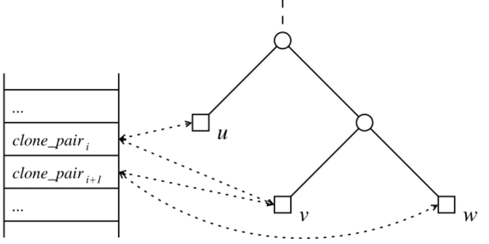
Every external node of the suffix tree stores references to the clone pairs of which a fragment relates to this node. On the other hand, every clone pair maintains links to the two nodes to which its fragments correspond. These bi-directional links are exploited whenever the structure of the suffix tree is modified andIDArequests all fragments relating to an external node. When external nodes are removed from the suffix tree due to the corresponding suffixes being deleted, fast access to the clone pairs is required, because these need to be changed. Note, that each clone pair is linked to exactly two nodes, whereas each node can be linked to an arbitrary number of clone pairs. Figure 10 shows how pairs and external nodes are linked.
u
v w
clone_pair clone_pair ...
...
i
i+1
Figure 10 – Schematic view of bi-directional links (dotted ar- rows) between external nodes and the fragments of clone pairs.
clone pairihas one fragment related to nodeuand the other frag- ment related to nodev. Likewise,clone pairi+1’sfragments relate to nodesv andw.
3.2.1 Tree Construction
Unfortunately, the construction methods for suffix trees that are imple- mented in clones, are not flexible enough to allow for fast insertion and deletion of strings into a generalized suffix tree. IDA implements unpa- rameterized clone detection, because the impact of adding or removing a parameterized string from a parameterized generalized suffix tree has not been evaluated within this thesis. This makes Baker’s constructor for pa- rameterized suffix trees unusable forIDA. The constructor that implements Ukkonen’s algorithm is also not usable, as it processes a single string on- line from its first to its last character. The benefit of being on-line is not required in our application, as parts of the string do change after they have been processed once.
Instead,IDA’s tree construction is based onMcCreight’salgorithm [McC76].
McCreight was the first to give a comparatively simple algorithm for con- structing a suffix tree in linear time. In contrast to Ukkonen’s algorithm, suffixes are added from longest to shortest to the tree. While construct- ing the tree, suffix links are created and exploited in later iterations. The drawback of McCreight’s algorithm is, that it operates “backwards” start- ing with the longest suffix. This means the whole string has to be known upon starting the algorithm. Nonetheless, this method is used by IDA to construct and modify the suffix tree. There is no problem in starting with the longest suffix, because the program’s source code is completely available upon starting the clone detection. Furthermore,McCreight’s algorithm can easily be applied to generalized suffix trees.
However, IDA does not follow McCreight’s original paper, but a simplified version which is described by Amir et al. [AFG+93]. Amir et al. present two procedures. One of them inserts a suffix of a string into the (general- ized) suffix tree and the other one accordingly deletes a suffix from the tree.
Assuming that all suffixes of a string are added or deleted (and not a single one on its own), both procedures take constant time. The assumption is valid for IDA, because whenever a file is changed, all its suffixes are added or deleted. A string of lengthm, which can be seen as a file withm tokens, has m suffixes and can therefore be added or deleted from the suffix tree and its underlying set of strings ∆ in linear time O(m). Like with other constructors, the generalized suffix tree is augmented with suffix links. A brief explanation of both procedures is given. A detailed description and a proof why they require linear time can be found in [AFG+93].
Inserting a Suffix: Inserting a suffix of a string into the generalized suffix tree is done by creating a new external node representing that suffix together with a new external edge. The challenge is to identify the location where the
new edge is to be appended. This is done by following the edges away from the root as long as the tokens represented by the edge labels correspond to the tokens of the suffix. There is only one such path, because the edge labels of sibling edges all start with a different token. When a discrepancy is found between the token referred to by an edge label and the corresponding token of the suffix, the location for inserting the new external edge and node has been found.
If the discrepancy was caused by the first token of an edge, the new external edge and its end node can be appended to the parent node of that edge.
Otherwise, the existing edge needs to be split by inserting a new internal node to which the new external edge must be appended. The new external edge label refers to the remaining tokens of the suffix for which no match has been found. Figure 11 shows both situations.
u
ab
c
d$
g ef
v
(a)Appending to an existing node.
e f u
ab
c g
$ v
(b) Splitting an edge.
Figure 11– Appending a new external node and edge to the suffix tree. Assuming the suffix to be added isabcd$, the new edge and node (dashed) can be appended to node u (a). If the suffix is abce$, the edge from node utov needs to be split. The new edge is appended to the newly created internal node (b).
During the process of inserting suffixes, suffix links are created. By using these links, the search does not need to be started from the root node for each remaining suffix. Instead, an internal nodes serves as the starting point for the search to avoid redundant calculations and ensure linear time consumption for inserting all suffixes of a given string.
Deleting a Suffix: Deleting a suffix is similar to adding one. It implies deleting an existing external node and its parent edge. Finding the node that is to be deleted works analogous to finding the location where a new node is to be appended. Starting from the root, edges are traversed as long as the tokens referenced by their labels equal the tokens from the suffix that is to be deleted. The search ends at the external node that represents the suffix. Again, two situations can arise. If the parent node of the external node is the start node of more than two edges, the external node and its external parent edge can be removed. If the external edge has only one sibling, the sibling and the parent edge of its start node have to be merged after removing the external edge. This is required, because no node except for the root can be the start node of only one edge.
Merging two edges is the opposite of splitting them. Coming back to Figure 11 and assuming the dashed parts to be deleted, subfigure (a) requires no further modification of the tree. When the dashed edge is removed from subfigure (b), its start node remains the start node of only one other edge.
This requires merging the edges fromu to the start node and from the start node tov.
IDA always deletes suffixes from longest to shortest. If the external node representing the longest suffix has been found, any other node representing a shorter suffix of the same string can be retrieved by following the suffix links. This means, every following suffix can be deleted in constant time.
3.2.2 Updating Labels
There is a serious problem in modifying generalized suffix trees after their initial construction. One should recall that every edge is labeled by a triple consisting of file, start and end referring to a substring of tokens. Consid- ering this, deleting files might result in edges, whose labels point to files which are not existent any more. A solution to this problem is described by Ferragina et al. [FGM97]. They make the following statement about labels:
“[. . . ] a label (X, i, j) is consistent if and only if it refers to a string currently in ∆.” [FGM97]
Using this definition, every label of a generalized suffix tree must be consis- tent at any point of time. Ferragina et al. identify three basic operations that modify the structure of the suffix tree.