Non-perturbative lattice approaches to complex path integrals: from non-perturbative saddle points to real-time physics of chiral media

(1)

Non-perturbative lattice approaches to complex path integrals: from non-perturbative saddle points to

real-time physics of chiral media

DISSERTATION

zur Erlangung des Doktorgrades der Naturwissenschaften (Dr. rer. nat.) der Fakultät für Physik der Universität Regensburg

vorgelegt von

Semen Valgushev

aus Ulyanovsk, Russland

Regensburg, Oktober 2018

(2)

Die Arbeit wurde von Dr. Pavel Buividovich angeleitet.

Das Promotionsgesuch wurde am 28.06.2017 eingereicht.

Das Promotionskolloquium fand am 04.12.2018 statt.

Prüfungsausschuss:

Vorsitzender: Prof. Dr. Christoph Strunk

1. Gutachter: Dr. Pavel Buividovich

2. Gutachter: Prof. Dr. Vladimir Braun

weiterer Prüfer: Prof. Dr. John Schliemann

(3)

Publications

The list of publications related to this thesis is the following:

[1] P.V. Buividovich, Gerald V. Dunne, and S.N. Valgushev. “Complex Path Integrals and Saddles in Two-Dimensional Gauge Theory”. Phys. Rev. Lett. 116 (2016), 132001. arXiv: 1505.04582 .

[2] P.V. Buividovich, M. Puhr, and S.N. Valgushev. “Chiral magnetic conductivity in an interacting lattice model of parity-breaking Weyl semimetal”. Phys. Rev. B 92 (2015), 205122. arXiv: 1505.04582.

[3] P.V. Buividovich and S.N. Valgushev. “Lattice study of continuity and finite- temperature transition in two-dimensional SU(N ) × SU (N ) Principal Chiral Model”. Submitted to Phys. Rev. D (2017). arXiv: 1706.08954.

[4] M.V. Ulybyshev and S.N. Valgushev. “Path integral representation for the Hub- bard model with reduced number of Lefschetz thimbles” (2017). arXiv: 1712.

02188.

[5] P.V. Buividovich and S.N. Valgushev. “First experience with classical-statistical real-time simulations of anomalous transport with overlap fermions”. PoS LAT- TICE (2016), 253. arXiv: 1611.05294.

[6] S.N. Valgushev, M. Puhr, and P.V. Buividovich. “Chiral Magnetic Effect in finite- size samples of parity-breaking Weyl semimetals”. PoS LATTICE (2015), 043.

arXiv: 1512.01405.

(6)

(7)

Acknowledgments

I would like to thank my supervisor Dr. Pavel Buividovich for giving me opportunity to work on exciting problems here, in Regensburg, and for guiding me.

Many thanks go to my wonderful colleagues Makism Ulybyshev, Oleg Kochetkov, Arthur Dromard, Matthias Puhr and Ali Davody. Creative and pleasant atmosphere of our group has always encouraged and inspired me.

I would like to especially thank Gerald Dunne for very exciting collaboration and his support. I am grateful to Mithat Unsal, Alexei Cherman, Tin Sulejmanpasic, Ariel Zhitnitsky, Dmitri Kharzeev, Edward Shuryak, Leonid Glozman, Alexander Turbiner, Victor Braguta and Andrey Kotov for very interesting and fruitful discussions.

I indebted to my brother and mother for their unconditional support and belief in me.

Without their endless support this work would have never been done. I am also grateful

to all my friends who stayed with me, encouraged me when things seemed gloomy and

shared my bright days.

(8)

(9)

Chapter 1 Introduction

According to modern scientific knowledge, there are four types of force governing the matter in the Nature: electromagnetic, weak, strong and the gravity. Description of the first three ones is based on the principles of quantum field theory (QFT) and is summarized in a gauge theory known as the Standard Model. Physics of electromagnetic and weak forces is relatively well understood since in many physically important cases (but not in all) interactions are sufficiently weak such that one can use well-developed methods of perturbation theory. In the case of strong force situation is drastically different.

Theory of strong force, the Quantum Chromodynamics (QCD), is non-Abelian gauge theory which is believed to describe rich phenomenology of hadrons (protons, neutrons, pions, etc.) and their interactions. The fact that gauge symmetry is non-Abelian implies that QCD is asymptotically free theory [1, 2]: interaction strength tends to vanish in the limit of very high energies. Thus theory becomes effectively free and some problems can be systematically studied with the help of perturbation theory in high energy regime.

On the other hand, in the domain of low energy physics, which is in many respects the most interesting one, the coupling constant becomes large and standard perturbative approach is not applicable. Due to breakdown of perturbation theory which happens at the dynamically generated strong scale Λ, finding a reliable approach to such system is major theoretical problem nowadays.

Multiple experimental evidences such as Bjorken scaling in high energy collisions

confirm asymptotically free nature of the strong force and physical existence of quarks

and gluons in terms of which QCD Lagrangian is formulated. However, neither quarks

nor gluons have ever been observed directly in experiments. The reason for that is that

quarks are always confined inside hadrons (which are bound states in QCD) due to strong

attractive force between them. This phenomenon is known as confinement. Observable

properties of hadron spectra are consistent with existence of some sort of string stretched

between quarks [3, 4], such that energy of the string growths with the distance and quarks

cannot be separated apart. The tension of the string extracted from experimental data is

(10)

√ σ ≈ 440MeV. The phenomenon of quark confinement cannot not be seen at any order of perturbation theory due to large characteristic distances comparable to typical hadron radius r ∼ 1fm or, in other words, due to small involved momenta smaller that QCD strong scale Λ

_QCD

∼ 1 GeV.

Due to strongly interacting nature of QCD properties of even lightest hadrons cannot be analytically calculated from the first principles. Since hadrons are basic excitations of strong interactions this causes serious difficulties in all spectrum of related phenomeno- logical problems, ranging from high energy particle collisions and nuclear physics to astrophysics and cosmology. One of the most important is the problem of studying equation of state and phase diagram of hadronic matter at different temperatures, densities and pressure. This question is deeply related to the problem of confinement: when system of baryons and mesons is heated up to temperatures comparable to QCD strong scale T

c

∼ Λ

QCD

it undergoes a deconfinement phase transition after which hadrons “melt down” and quarks and gluons are liberated. This new state of matter is called Quark Gluon Plasma (QGP) which is a subject of intense experimental study in modern heavy ion collision experiments at RHIC and LHC, see [5, 6] for a review. Failure of perturbation theory in describing low energy physics is related to deconfinement phase transition:

an appropriate choice of degrees of freedom for describing quarks confined in hadrons would be some sort of string-like collective excitations which bind them together whereas perturbation theory operates in terms of point-like quarks and gluons. Degrees of freedom undergo deep reorganization at the strong scale which is reflected in the presence of the phase transition.

1.1 Goals

This Thesis is an attempt to find a key, an approach, which would allow to understand details of strongly coupled dynamics of asymptotically free theories such as QCD. The source of our inspiration is the observation that non-perturbative phenomena and per- turbative expansions are tightly related to each other in a very non-trivial way, so that a complete description of a quantum theory is only possible when both “sectors” are taken into account simultaneously. Such relations is a central subject of the resurgence theory.

One of the leitmotifs of this theory is the appreciation of physically important role of unstable, non-topological and even complex saddle points of path integrals.

1.1.1 Asymptotically free theories and resurgence theory

Resurgence theory has recently provided new insights into matrix models and string

theories [7–12], and has been applied to asymptotically free QFTs and sigma models

[13–16], and localizable SUSY QFTs [17]. It appears that aforementioned classes of

(11)

saddle points are important for consistent semi-classical description of asymptotically free theories and in the most dramatic scenarios can even be responsible for phase transitions.

Such saddles naturally appear in the semi-classical expansion in the framework of the Lefschetz thimble decomposition of the path integral [18, 19].

The Lefschetz thimbles decomposition can be obtained by deforming integration contour of the path integral into extended, complex space. Mathematical Morse theory, or Picard-Lefschetz theory, suggests that it is possible to construct such manifold in the complex plane that the path integral is decomposed as:

Z (λ) = X

σ

k

_σ

(λ) Z

_σ

(λ) , (1.1)

Z

_σ

(λ) = ˆ

I_σ(λ)

D[x]e

^−S(λ,x)

, (1.2) where σ labels complex saddle points z

_σ

(λ) ∈ C of the action, coefficients k

_σ

(λ) ∈ Z are so-called intersection numbers and I

_σ

(λ) are real steepest descent manifolds, or Lefschetz thimbles, originating from σ-th saddle point. One can also define a dual real steepest ascend manifold, or anti-thimble K

σ

, which ends up at the given saddle point.

With the help of anti-thimbles one can compute integer-valued coefficients k

_σ

in the expression (1.1) by counting the (oriented) number of intersection of K

_σ

with original integration contour of the path integral. Due to to the fact that imaginary part of the action is constant on both thimble and anti-thimble, one can consider Lefschetz thimbles decomposition as a multi-dimensional generalization of the stationary phase method.

We note that all quantities in the equation (1.1) depend non-trivially on parameters λ. Moreover, the structure of thimbles I

_σ

and anti-thimbles K

_σ

can significantly change as λ is varied, so that Stokes phases are correctly taken into account. In particular, intersection numbers k

σ

can jump due to movement of anti-thimbles, so that some thimble integrals will appear and some will disappear from the sum (1.1). This is a non-trivial topological manifestation of the fact that contributions of different saddle points are related to each other due to monodromy properties of the path integral as integration runs around singularities.

The connection of non-perturbative saddle points discussed above is reflected in the structure of asymptotic perturbative expansion. Resurgence theory generalizes ordinary perturbative series in powers of some small parameter g

²

to resurgent trans-series:

h O i =

∞

X

n=0

F

_n,0⁽⁰⁾

g

²ⁿ

+

∞

X

n=0

∞

X

k=1 k−1

X

l=1

F

_n,l^(k)

g

²ⁿ

exp

− A g

²

k

ln

± 1 g

²

l

, (1.3)

where exponential factors take into account non-perturbative effects, logarithms take into

account contributions of quasi-zero modes and corresponding power series of g

²

describe

local quantum fluctuations about the k-th saddle point. Trans-series are called resurgent

since the object which is represented by such series “surges up”, or resurrects, due to

(12)

mechanism of Brezin-Zinn-Justin (BZJ) ambiguity cancellation: Borel resummation of perturbative series about vacuum or k-th saddle point often requires careful regularization due to appearing poles, especially in asymptotically free theories. Regularization, how- ever, leads to exponentially small ambiguities (since poles can be by-passed from below or above), which are exactly cancelled by certain non-perturbative amplitudes, e.g. due to instanton-anti-instanton transitions, which also become ambiguous when regularization is applied. Thus, resulting resummed expression appears well-defined and at the same time takes into account both perturbative and non-perturbative phenomena.

The structure of BZJ cancellation implies that expansion coefficient F

_n,l^(k)

are highly correlated and that perturbative series actually contains important information about non-perturbative physics. This information is particularly encoded in the location and residues of the aforementioned poles. The most well known example of such pole is infrared renormalon in non-Abelian gauge theory [20–28], see also review [29]. The renormalon appears if one tries to resum important class of Feynman diagrams, so-called

“bubble chains”, which take into account effect of the running coupling (thus, renormalon is related to renormalization). It is believed that infrared renormalon is tightly related to non-perturbative physics responsible for mass gap generation in non-Abelian gauge theory [20–28].

A complete study of resurgent relations of perturbative and non-perturbative physics is only possible for systems where one can compute any term of the expansion and/or find all saddle points and Lefschetz thimbles. Unfortunately, only very limited information is available in realistic theories. An important step towards realistic systems can be made with the help of special deformations which could bring asymptotically free theory from strongly coupled into weakly coupled regime in a controllable way. For instance, one can make one spatial direction compact and impose specific boundary conditions, so-called Z

N

-symmetric twist [14–16, 30, 31]. When the size of compact direction is large, effect of the twist should be negligible, whereas at very small size the theory should become weakly coupled due to asymptotic freedom. The purpose of the twist is to suppress possible phase transition from confined into deconfined phase as the size L of the compact direction is varied from large to small values. If this phase transition is suppressed, then one can perform computations in weakly coupled regime at small L and after analytically continue them into strongly coupled regime at large L. The conjecture that deconfinement phase transition is suppressed is called adiabatic continuity conjecture.

It is important to study this conjecture since it is a cornerstone ingredient for resurgence

studies of two dimensional asymptotically free models where one can find interpretation

of renormalon divergence in terms of (unstable) saddle points, which at the same time are

responsible for the mass gap generation [14–16, 30, 31]. It is also very important in the

light of recent program of applying similar ideas directly to Yang-Mills theory and QCD

[32, 33].

(13)

In this Thesis we investigate the physical role of non-pertubative phenomena in several problems in the context of resurgence theory. To this end we employ lattice field theory for regularization of the path integrals which allows us to obtain results from first principles with the help of numerical Monte-Carlo simulations and to consider phenomena which cannot be tested by other means.

1.1.2 The sign problem

We are also interested in studying physical origins of so-called sign problem in Monte- Carlo simulations: numerical simulations are based on algorithms of importance sampling where field configurations are generated randomly according to distribution given by the Boltzmann weight e

^−S

in the path integral. It is crucial that the action S is real, so that Boltzmann weight can be interpreted as probability density function. However, this is not the case if a system with fermions is considered at the finite chemical potential since fermionic effective action becomes complex with highly oscillating phase. Because of the sign problem it is very challenging to study the phase diagram of QCD at finite density, see reviews [34, 35]. Since the problem affects basically any physical systems with fermions at finite density, we choose two dimensional Hubbard model [36, 37] which is physically very interesting and, at the same time, allows to simplify analysis compared to QCD. It can serve as a model of high-temperature superconductor where superconducting phase is expected to exist at large values of chemical potential [38–40]. In our work we explore an approach to the sign problem based on Lefschetz thimble decomposition. The idea is motivated by the fact that imaginary part of the action is constant on the thimble manifold, thus partition function is given by a sum of integrals each of which can, in principle, be approached by standard Monte-Carlo techniques.

1.1.3 Transport properties of chiral fermions and real-time simulations

Finally, we are interested in studying novel transport phenomena appearing in systems with chiral fermions due to presence of quantum axial anomaly. The axial anomaly, or Adler-Bell-Jackiw (ABJ) anomaly [41, 42], is probably one of the best know ways to relate perturbative and non-perturbative physics:

∂

_µ

j

₅^µ

= − N

_f

16π

²

F

_µν

F ˜

^µν

, (1.4)

where j

₅^µ

= ¯ ψγ

^µ

γ

⁵

ψ is axial current, F

_µν

= ∂

_µ

A

_ν

− ∂

_ν

A

_µ

is the stress-tensor of a

(non-Abelian) background gauge field, F ˜

^µν

=

¹₂

^µναβ

F

_αβ

is a dual stress-tensor and N

_f

is number of fermion flavors (N

_f

= 3 in QCD). On the one hand, this equation is exact

perturbative result [43]. On the other hand, in the case of non-Abelian gauge theory the

(14)

quantity of the r.h.s. of this equation is a total derivative of topological Chern-Simons current K

^µ

, so that the change of the fermionic axial charge over time ∆Q

₅

is related to topological Chern-Simons number Q

CS

=

_32π^N^f2

´ d

⁴

x ∂

µ

K

^µ

of gauge fields:

∆Q

5

= 2Q

CS

. (1.5)

Thus, in non-Abelian gauge theory fermionic currents reveal non-trivial topological prop- erties of the vacuum. However, even in Abelian case it can have far going consequences.

Axial anomaly drives unusual dissipation-less transport which is often referred to as anomalous transport. These effects have multiple manifestations in rich variety of situations ranging from particle [44–46] and condensed matter physics [47–49] to processes in astrophysics and at cosmological level [50–54]. It appears in media which violate P and CP symmetries in one of the possible ways: e.g. one can consider a medium with different number of left and right handed fermions, or consider non-Abelian gauge theory where spaleron transitions can induce local fluctuations of axial charge. A combination of such medium and external magnetic field gives rise to Chiral Magnetic Effect (CME) [45]:

j = σ

_{CM E}

B, (1.6)

where j is electric current and σ

_{CM E}

is so-called chiral magnetic conductivity which is supposedly protected from renormalization due to tight connection to the axial anomaly.

In particular, since nuclei in heavy-ion collisions can create very large magnetic fields eB ∼ m

²_π

[55] at the first moments of collision, CME can lead to detectable fluctuations of electric charge asymmetry.

In order to describe anomalous transport it is necessary, however, to go beyond tradi- tional equilibrium paradigm. It is by now commonly accepted that anomalous transport phenomena cannot exist in equilibrium [56], and moreover, at certain circumstances axial anomaly and CME can even drive so-called Chiral Plasma Instability [57] which is expected to play important role in astrophysics and cosmology. Also, in the case of heavy ion collision experiments the expected life-time of strong magnetic field, which is the moment when anomalous effects receive main contributions, is so short (t ≈ 1f m/c [55]) that it poses a question whether quark gluon plasma really succeeds to thermalize within such a short time [58].

Real-time problems are notoriously difficult. From the point of view of first principle

numerical computations, they represent an extreme case of the sign problem which can

be addressed only on future quantum computers. At the present moment, it is necessary

to employ simplifying approximations in order to address realistic problems. In the

present work, we use so-called classical-statistical field theory (CSFT) approximation,

which helps to capture essential non-perturbative effects such as particle pair production,

combined with lattice field theory for studying anomalous transport properties of chiral

(15)

fermions in non-stationary environment. We are especially interested in studying the performance of overlap fermions, which realize exact lattice chiral symmetry, in real-time simulations.

1.2 Outline

The rest of the thesis is organized as follows:

• In the Chapter 2 we study saddle points structure of two-dimensional lattice gauge theory represented as Gross-Witten-Wadia (GWW) unitary matrix model in the context of the resurgence theory. We express the path integral in terms of fields analytically continued into complex plane in order to explore the physical role of complex saddle points. In the weak coupling phase, we confirm a conventional mechanism of instanton gas condensation which drives the 3rd-order N = ∞ phase transition from weak to strong coupling regime. In the strong coupling phase we find a new interpretation of non-perturbative effects in terms of complex saddle points which are obtained by “eigenvalues tunneling” into complex plane. The action of these new saddle points matches predictions of the resurgence theory analysis of the 1/N expansion of the free energy.

• In the Chapter 3 we study two-dimensional SU (N ) × SU (N ) Principal Chiral Model (PCM) using first-principle lattice simulations. PCM is a confining asymp- totically free quantum field theory which can be considered as a toy model of QCD. We explore the validity of adiabatic continuity conjecture and effect of Z

_N

-symmetric twist on the phase structure and non-perturbative features of PCM.

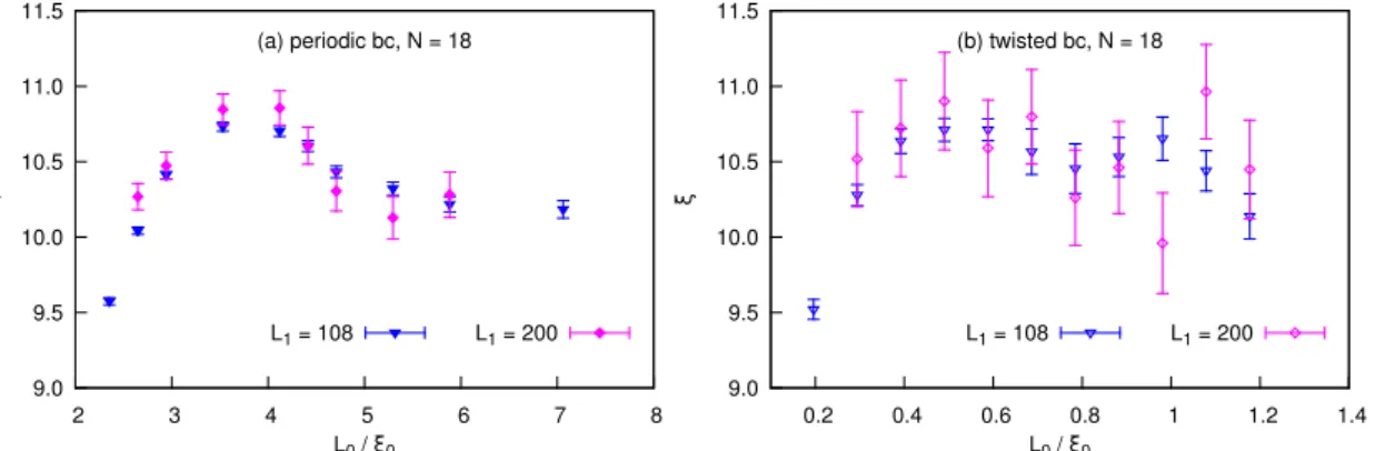
In our work we use lattices of the size L

0

× L

1

, where the twist is imposed on the 0-th direction. We compare our result to simulations of PCM with periodic boundary conditions where L

₀

can be considered as inverse temperature. For both boundary conditions our numerical results can be interpreted as signatures of a weak crossover or phase transition at N = ∞ between the regimes of small and large L

₀

. In particular, at small L

₀

thermodynamic quantities exhibit nontrivial dependence on L

₀

, and the static correlation length exhibits a weak enhancement at some “critical” value of L

₀

. We also observe important differences between the two boundary conditions, which indicate that the transition scenario is more likely in the periodic case than in the twisted one. In particular, the enhancement of correlation length for periodic boundary conditions becomes more pronounced at large N, and practically does not depend on N for twisted boundary conditions.

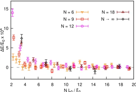
Furthermore, using Gradient Flow we study non-perturbative physics of the theory

and find that enhancement of the correlation length appears when the length L

₀

becomes comparable with the typical size of unitons, unstable non-topological non-

(16)

perturbative saddle points of PCM. With twisted boundary conditions these saddle points become effectively stable and one-dimensional in the regime of small N L

₀

, whereas at large N L

0

they are very similar to the two-dimensional unitons with periodic boundary conditions. In the context of adiabatic continuity conjecture for PCM with twisted boundary conditions, our results suggest that while the effect of the compactification is clearly different for different boundary conditions, one still cannot exclude the possibility of a weak crossover separating the strong-coupling regime at large N L

₀

and so-called Dunne-Ünsal regime at small N L

₀

with twisted boundary conditions.

• In the Chapter 4 we study the sign problem in two-dimensional Hubbard model at non-zero chemical potential (away from half-filling regime) through the prism of Lefschetz thimble decomposition of the path integral. In this approach the sign problem can be reduced if partition function can be represented as a sum over Lefschetz thimbles with only a few different global phases. We explore the complexity of the sign problem in the few-site Hubbard model on square lattice with the help of semi-analytical study of saddle points and corresponding Lefschetz thimbles. Due to complexity of the problem, we employ small lattices with several steps in the direction of imaginary Euclidean time. We study different variants of the Hubbard-Stratonovich transformation of the interaction term and find representation where a minimal number of thimbles contribute to the partition function in the vicinity of half-filling: there are only two relevant thimbles on few-site lattice in this regime. We also find indirect evidence that this regime can exist in more realistic systems with large sizes. Finally, we derive a novel non-Gaussian representation of the interaction term, where the number of relevant Lefschetz thimbles is significantly reduced in comparison to conventional Gaussian Hubbard-Stratonovich transformation.

• In the Chapter 5 we present first results of classical-statistical real-time simulations

of transport phenomena of chiral fermions modelled by overlap fermions. We find

that even on small lattices overlap fermions reproduce the real-time anomaly equa-

tion with much better precision than Wilson-Dirac fermions on significantly bigger

lattices. The difference becomes much more pronounced for quickly changing

electromagnetic fields, especially if one takes into account the back-reaction of

fermions on electromagnetic fields. As test cases, we consider chirality pumping

in parallel electric and magnetic fields and mixing between the plasmon and the

Chiral Magnetic Wave.

(17)

Chapter 2

Complex saddle points in two-dimensional gauge theory

2.1 Introduction

In gauge theories, there are two physical parameters which control the strength of fluctua- tions around the saddle points and enter the resurgent trans-series expansion: the rank N of the gauge group and the t’Hooft coupling λ ≡ N g

²

, with gauge coupling g

²

[59]. The interplay between the dependence on N and λ leads to novel effects [7, 8, 12] which we explore here. An important goal would be to construct uniform resurgent approximations [60] (with respect to λ and 1/N ) which analytically relate the weak and strong coupling phases. For gauge theories, such a relation would certainly improve our understanding of confinement and dynamical mass gap generation. It would also extend the applicability of Diagrammatic Monte-Carlo studies of non-Abelian lattice gauge theories, which are so far limited to the regime of unphysically strong bare coupling constants [61].

The difference between weak and strong coupling phases is particularly dramatic in

the large-N limit of 2D gauge theories, where they are separated by a third-order phase

transition with respect to the t’Hooft coupling λ [62–65] and/or the manifold area A [66,

67]. Physically, on the weak coupling side this large-N phase transition in 2D gauge

theory is related to the condensation of instantons [65, 67, 68], which are exponentially

suppressed at large N away from the transition point. Much less is known about the role

of instantons (or other saddles) on the strong coupling side of this transition, except in the

double scaling limit. Here we study the simplest example of 2D lattice gauge theory, the

Gross-Witten-Wadia unitary matrix model [62–64], to demonstrate the novel properties

of complex saddles in the strong coupling phase as well as their relation to the resurgent

structure of the 1/N expansion.

(18)

2.2 Gross-Witten-Wadia (GWW) model

Gross-Witten-Wadia (GWW) model [62, 63] is a matrix model representation of two- dimensional U (N ) lattice gauge theory which is given by standard action:

S

_lat

= 1 g

²

X

x

Tr P

_x

, P

_x

= U

_x,0

U

_x+e₀_,1

U

_x+e^†

1,0

U

_x,1^†

, (2.1) where U

_x,µ

∈ U (N ) are lattice gauge fields, P

_x

is a plaquette operator and e

_µ

is a unit lattice vector in direction µ = 0, 1. In order to derive partiton function of the GWW model one can use gauge freedom and choose axial gauge in which fields in direction µ = 0 are all equal to identity U

_x,0

= 1, so that lattice action becomes S

_lat

= 1/g

²

P

x

Tr [U

x,1

U

_x+e^† ₀_,1

]. With the help of invariance of the Haar measure of the lattice path integral with respect to shifts d[U ] = d[W U ], where W ∈ U(N ), one can make a change of variables:

U

_x+e₀_,1

= W

_x

U

_x,1

, (2.2)

after which the partition function of the 2D lattice gauge theory takes a simple form:

Z

_lat

= ˆ

Y

x

d[U

_x,1

] e

^−S^lat

= (2.3)

= ˆ

Y

x

d[W

x

] exp

− N

λ Tr [W

x

+ W

_x^†

]

,

where λ = N g

²

is t’Hooft coupling. Hence, partition function factorizes: Z

lat

= Z

^V

, where V is lattice volume and Z is desired partition function of the GWW matrix model:

Z = ˆ

d[W ]exp

− N

λ Tr [W + W

^†

]

. (2.4)

Thus, all properties of two-dimensional lattice gauge theory can be obtained from a GWW matrix model.

Partition function (2.4) can be expressed in terms of phases z

_i

of eigenvalues e

^izⁱ

of unitary N × N matrix W :

Z =

N

Y

i=1

ˆ

π

−π

dz

i

e

^−S(zⁱ⁾

, S (z

i

) = X

i

V (z

i

) − ln ∆

²

(z

i

) ,

V (z) = − 2N

λ cos (z) , ∆ (z

_i

) = Y

i<j

sin

z

_i

− z

_j

2 . (2.5)

We are interested in the t’Hooft limit: N → ∞, g

²

→ 0 while λ = N g

²

is kept fixed. In this limit one can introduce normalized density of eigenvalues ρ(z) defined on the unit circle Re z ∈ [−π, π), Im z = 0:

N ρ(z)dz = dn, ˆ

π

−π

ρ(z) dz = 1, (2.6)

(19)

where dn is number of eigenvalues in the segment [z, z+dz]. The action (2.5) is expressed in terms of ρ(z) as:

S N

²

= 2

λ ˆ

π

−π

dz ρ(z) cos(z)− (2.7)

− 1 2 P.V.

ˆ

π

−π

dz ˆ

π

−π

dz

⁰

ρ(z)ρ(z

⁰

) ln

sin

²

z − z

⁰

2 ,

where P.V. refers to Cauchy principle value of the integral. It is clear that one can use N

²

as large parameter and perform saddle point analysis of the path integral. Leading saddle point contribution would correspond to planar limit of the 1/N expansion.

At N = ∞ this model has a third-order phase transition at λ

_c

= 2, where the third derivative of the free energy is discontinuous [62, 63]. In order to see this one can consider saddle points of the least action (vacuum fields) given by the following expressions [62, 63]:

ρ

^(w)

(z) = 2

λπ cos z 2

r λ

2 − sin

²

z 2

, λ < 2 (2.8) ρ

^(s)

(z) = 1

2π

1 + 2

λ cos (z)

, λ > 2. (2.9)

In the weak coupling phase λ < 2 the distribution ρ

^(w)

(z) has a support on semi-circle z ∈ [−z

_c

, z

_c

], where z

_c

is a solution to the equation sin

²

(z/2) = λ/2. Hence there is gap in the distribution so that eigenvalues do not occupy the whole unit circle. However, at the critical point λ = λ

_c

the gap in the distribution closes and eigenvalues can occupy any point of the unit circle in the strong coupling phase λ > 2. Explicit computation of the leading saddle point contribution yields the following result for the planar free energy:

E

₀

(λ) = − ln Z/N

²

= (2.10)

=







1

λ²

, λ > 2,

2

λ

+

¹₂

ln

^λ₂

−

³₄

, λ < 2 .

Third derivative of E

₀

(λ) is discontinuous at λ

_c

= 2, hence there is a phase transition of the third order.

2.3 Complex Saddle Points in the GWW model

In this Section we study saddle points of GWW model in the complex plane. In order to find saddle configurations with a priori unknown properties we numerically solve saddle point equations at large but finite N :

∂S

∂z

_i

= 0, (2.11)

(20)

where z

_i

∈ C . Complex eigenvalues can be visualized on the cylinder S

¹

× R , where S

¹

is the original unit circle and R is the imaginary direction.

Since the action S (z) of the GWW model is a holomorphic function of eigenvalues z

_i

, equations (2.11) can be solved with the help of e.g. Newton iterations. However, in our case the Newton iterations turned out to be unstable in the strong coupling phase for N larger than certain value N > 20. Because of that, we employed the Halley method which is next-order improvement of Newton iterations. We describe it in the Appendix A.1. Using this method we were able to solve the saddle-point equations for the values of N up to N = 400. As initial conditions for the Halley iterations we chose values z

_i⁽⁰⁾

randomly distributed in the rectangle Re z

_i

∈ [−π, π), Im z

_i

∈ [−5.0, 5.0], which yielded sufficiently many distinct solutions. We distinguish solutions up to the obvious symmetry of arbitrary permutations of eigenvalues z

i

.

2.3.1 General features

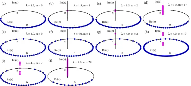
We find that all saddle points consist of (N − m) real eigenvalues located on the unit circle Re z ∈ [−π, π), Im z = 0, whereas m eigenvalues reside on the line z = π + iy, y ∈ R . We note that both the unit circle and the second complex line are the steepest ascent contours of the potential V (z) originating from its extrema at z = 0 and z = π.

The configurations of z

_i

are all symmetric with respect to these points. Hence, when m is odd there is always one eigenvalue located exactly at z = π. Some illustrative examples of found saddle points are presented on the Fig. 2.1 for different values of λ and m.

λ = 1.5, m = 0

0 π Re(z)

Im(z)

(a) λ = 1.5, m = 1

0 π Re(z)

Im(z)

(b) λ = 1.5, m = 2

0 π Re(z)

Im(z)

(c) λ = 1.5, m = 17

0 π Re(z)

Im(z)

(d)

λ = 4.0, m = 0

0 π Re(z)

Im(z)

(e) λ = 4.0, m = 1

0 π Re(z)

Im(z)

(f) λ = 4.0, m = 2

0 π Re(z)

Im(z)

(g) λ = 4.0, m = 10

0 π Re(z)

Im(z) (h)

λ = 4.0, m = 7

0 π Re(z)

Im(z)

(i) λ = 4.0, m = 28

0 π Re(z)

Im(z)

(j)

Figure 2.1: Saddle point configurations of eigenvalues z

_i

in the weak-coupling (plots (a) - (d)), and in the strong-coupling (plots (e) - (j)) phases with different “instanton numbers”

m. N = 40 on all of the plots except for the plot (h), where we take N = 100 in order to illustrate the three-cut solution at large m and strong coupling.

We have checked that in both weak and strong coupled phases the saddle points

with m = 0 correctly reproduce known results for the planar (vacuum) distribution of

(21)

eigenvalues (2.8, 2.9). We present numerical eigenvalue distribution at sufficiently large N = 400 compared to theoretical results on the Fig. 2.2 for few values of λ from both phases. Hence, we observe a phenomenon of vanishing gap in the eigenvalue distribution at the critical point λ

_c

= 2 which drives the N = ∞ phase transition.

0.00 0.05 0.10 0.15 0.20 0.25 0.30 0.35 0.40

-3 -2 -1 0 1 2 3

ρ (z)

z

λ = 1.5 λ = 2.0 λ = 4.0

Figure 2.2: Numerical eigenvalue distributions for the m = 0 saddle [N = 400], com- pared with the analytic ρ (z) in (2.8, 2.9).

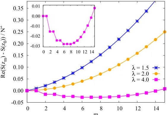
The real part of the action of saddle points is illustrated on the Fig. 2.3 as a function of m for several representative values of λ from both phases. The imaginary part of the action is always a multiple of π:

Im S (z) = πbm/2c, (2.12)

where b·c is the floor function. Thus, saddle point contributions e

^−S^m

to the path integral are always real, either positive or negative, although eigenvalues are manifestly complex.

This phenomenon can be interpreted as a hidden topological angle [69]. We note that it has the origin in the Vandermonde determinant ∆

²

(z).

2.3.2 Weak coupling phase

The leading non-perturbative saddle point at λ < 2 is the one with m = 1. It can

be obtained from the vacuum field configuration by dragging one eigenvalue from the

support of the ρ(z) to the point z = π, as depicted on the Fig. 2.1(b). The action of this

saddle, relative to the action of the vacuum m = 0, can be obtained analytically [8] with

the help of the following electrostatic analogy: all eigenvalues can be though as electric

(22)

-0.03 -0.02 -0.01 0.00 0.01

0 2 4 6 8 10 12 14

-0.05 0.00 0.05 0.10 0.15 0.20 0.25 0.30 0.35

0 2 4 6 8 10 12 14

Re(S(z

m

) - S(z

0

)) / N

2

m

λ = 1.5 λ = 2.0 λ = 4.0

Figure 2.3: Real part of the saddle action, Re S (z), versus instanton number m, for different values of λ, at N = 40. The inset shows Re S (z) vs m at λ = 4 on a larger scale.

charges placed in the external potential V (z) and repelling each other according to the Vandermonde term ln ∆

²

(z) in the action. One can compute the work needed to move a single charge from the support of ρ(z) to the point z = π in the background of the self-consisted electric field created by all other eigenvalues. The resulting N = ∞ action is the following:

S

_I^(w)

= 4/λ p

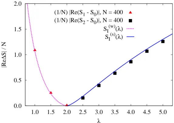
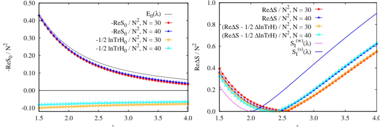
1 − λ/2 − arccosh ((4 − λ)/λ) , λ < 2. (2.13) We depict numerical action of m = 1 saddle at N = 400 compared to theoretical result on the Fig. 2.4. We observe a good agreement.

For larger m > 1 eigenvalues go into complex plane and arrange themselves along the line z = π + iy symmetrically with respect to the point z = π, see Fig. 2.1(c,d). We interpret this result as “eigenvalue tunneling” where tunneled eigenvalues are complex.

As N increases, eigenvalues clearly tend to form a cut.

We note that in the vicinity of the critical point λ → λ

c

the real part of the action of saddle points with sufficiently small m N scale approximately linearly with m:

Re (S

_m

− S

₀

) = m N S

_I^(w)

. Thus, one can identify m as number of weakly interacting

“instantons” (it is common to refer to such non-perturbative saddle points as instantons).

Hence we confirm a conventional picture of dilute instanton gas in the weak coupling

phase.

(23)

0.0 0.5 1.0 1.5 2.0

1.0 1.5 2.0 2.5 3.0 3.5 4.0 4.5 5.0

|Re ∆ S| / N

λ

(1/N) |Re(S ₁ - S ₀ )|, N = 400 (1/N) |Re(S ₂ - S ₀ )|, N = 400 S _I ^(w) ( λ ) S _I ^(s) ( λ )

Figure 2.4: Numerical results (dots) for the relative actions of the leading non-vacuum saddles with m = 1 (in the weak-coupling phase) and m = 2 (in the strong-coupling phase), at N = 400. Solid lines are the analytic expressions (2.13) and (2.15).

We also study the spectrum of the Hessian matrix:

H

_{m, ij}

= ∂

²

S

_m

∂z

_i

∂z

_j

, (2.14)

which describe Gaussian fluctuations about the m-th saddle point. We consider its properties in details in the Subsection 2.3.5. In particular, we find that in the weak coupling regime it has exactly m negative eigenvalues for the m-th saddle point, thus the m = 1 saddle point give an imaginary contribution to the saddle point expansion of the free energy. This imaginary contribution is cancelled by imaginary term from the Borel summation of divergent 1/N expansion about the m = 0 vacuum saddle point. Thus, we observe a clear indication of resurgent cancellations. This can be traced to the resurgent asymptotics of individual Bessel functions, using the determinant representation [62, 63]

of the partition function: Z = det (I

j−k

(2N/λ)) .

2.3.3 Phase transition and instanton condensation

As λ → 2 from the weak-coupling side, the gap in the eigenvalue distribution closes

at the point z = π, see Fig. 2.1 and Fig. 2.2. Furthermore, as seen on the Fig. 2.3, the

real part of the saddle action, relative to the vacuum value, tends to zero, so that all

instantons with m N become equally important at the transition point, signaling

instanton condensation [8, 65, 67].

(24)

2.3.4 Strong coupling phase

In the strong coupling phase λ > 2 the gap in the eigenvalue distribution is closed and the point z = π is already in the support of ρ

^(s)

(z). Because of that, non-vacuum saddles can no longer be constructed by dragging eigenvalues to z = π as it was possible in the weak coupling phase. Nevertheless, Mariño obtained the following strong-coupling “instanton action" using a trans-series ansatz in the string equation [8] (see also Appendix B in [70]):

S

_I^(s)

= 2arccosh (λ/2) − 2 p

1 − 4/λ

²

, λ ≥ 2. (2.15)

We find a natural interpretation of this “instanton” as a saddle configuration, with complex eigenvalue tunneling from the real to the imaginary axis (see Fig. 2.1). As in the weak coupling phase, m eigenvalues line up along the imaginary direction, but these strong- coupling saddles have some surprising properties.

Quasi-zero mode

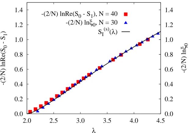
First of all, we find that at large N , the m = 1 saddle point has real action which differ from that of the m = 0 saddle up to exponentially small corrections precisely of the form:

Re (S

1

− S

0

) ∼ exp

−N/2 S

_I^(s)

, (2.16)

where S

_I^(s)

(λ) is the strong-coupling instanton action (2.15). We depict this difference on the Fig. 2.5. Physically, this is due to quasi-zero mode which emerge in the strong- coupling regime: in the limit λ → ∞ the potential V (z) becomes irrelevant and saddle point configuration is determined solely by the Vandermonde term ln ∆

²

(z) in the action (2.5). This term has an extra global U (1) symmetry: all eigenvalues can be rotated by an arbitrary angle simultaneously. The quasi-zero mode is an remnant of this extra symmetry at finite values of λ > 2, so that eigenvalue medium on the unit circle can support some sort of collective “sound wave”.

Because of the quasi-zero mode, the m = 0 and m = 1 configurations can be transformed into each other by the shift in the flat direction, so that they have the same continuous eigenvalue density, but microscopically differ by the presence or absence of a single eigenvalue at z = π, see Fig. 2.1, (e) and (f). The shift moves every eigenvalue to the middle of the interval to its neighboring eigenvalue. At large N this interval is inversely proportional to the density function ρ

^(s)

(z), so that flat direction is given by:

δz

_i

∼ 1

ρ

^(s)

(z

i

) . (2.17)

Direct substitution of this expression into the integral equation for eigenvectors of the

Hessian matrix (2.14) yields that δz is indeed an eigenvector with zero eigenvalue at

(25)

0.0 0.2 0.4 0.6 0.8 1.0 1.2 1.4

2.0 2.5 3.0 3.5 4.0 4.5

0.0 0.2 0.4 0.6 0.8 1.0 1.2 1.4

-(2/N) lnRe(S 0 - S 1 ) -(2/N) ln ξ 0

λ

-(2/N) lnRe(S ₀ - S ₁ ), N = 40 -(2/N) ln ξ ₀ , N = 30 S _I ^(s) (λ)

Figure 2.5: Comparison of the log of the difference between the actions of the m = 0 and m = 1 saddles (left vertical axis), and the log of the lowest Hessian eigenvalue ξ

₀

(right vertical axis), in the strong coupling phase, with half the strong coupling instanton action in (2.15). Both effects are governed by the same exponential.

N = ∞:

[Hδz] (z) = − 2

λ cos (z) δz (z) − P.V.

ˆ

π

−π

dz

⁰

ρ

^(s)

(z

⁰

) δz (z) − δz (z

⁰

)

sin

² ^z−z₂ ⁰

= 0, (2.18) where H is the Hessian operator and P.V. refers to the Cauchy principal value of the integral. Note that since δz (z) is analytic for z ∈ [−π, π], the integrand in the second term on the right-hand side of (2.18) diverges only as 1/z rather than 1/z

²

, thus the integral is well defined in the sense of Cauchy principal value.

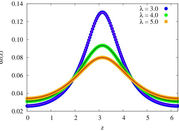
Furthermore, we numerically compute eigenvector δz which correspond to the lowest eigenvalue ξ

₀

of the Hessian at large but finite N = 400. On the Fig. 2.6 we demonstrate a good agreement between the numerical and theoretical result (2.17). We also find that as N → ∞, the lowest eigenvalue ξ

₀

vanishes exponentially fast as exp

−N/2 S

_I^(s)

, see Fig. 2.7 and Fig. 2.5. Interestingly, this is the same exponential factor seen in the splitting Re (S

₁

− S

₀

).

Strong coupling “instanton” saddles

In the strong-coupling phase, it is not the m = 1 saddle, but rather the m = 2 saddle which

we identify as the “strong-coupling instanton” configuration. This saddle is manifestly

(26)

0.02 0.04 0.06 0.08 0.10 0.12 0.14

0 1 2 3 4 5 6

δ z(z)

z

λ = 3.0 λ = 4.0 λ = 5.0

Figure 2.6: Comparison of the analytic expression δz ∼ 1/ρ

^(s)

(z) for the zero mode of the Hessian matrix H

₀

of the m = 0 saddle in the strong-coupling phase (solid line) with numerically calculated eigenvector of H

₀

which corresponds to the lowest eigenvalue at N = 400.

complex, see Fig. 2.1 (g). It has action with real part equal to, as a function of λ, the modulus of the strong-coupling action (2.15): |Re (S

₂

− S

₀

) | = N S

_I^(s)

(λ), see Fig. 2.4.

This reversal of sign is a numerical example of a phenomenon found in the context of the Painlevé equations, where formal trans-series arise with saddles of both signs of the action [10, 11, 71].

As m increases we find that eigenvalues continue to move to complex plane forming a two cut structure on the imaginary axis symmetric with respect to the point z = π, see Fig. 2.1 (g)-(i). If m is odd then there is always one eigenvalue exactly at the point z = π. When instanton number m reaches some critical value m

^?

the gap between two cuts on the imaginary axis closes and at the same time the gap in the distribution of real eigenvalues on the unit circle opens, see Fig. 2.1 (i),(j).

We find that the real part of the action decreases with m if m < m

^?

, see Fig. 2.3.

Furthermore, we find that the action of saddles m < m

^?

with instanton numbers m = 2n and m = 2n +1 exhibit quasi-degeneracy similar to that of saddles with m = 0 and m = 1 (note characteristic “stairs” on the inset of the Fig. 2.3). We also observe corresponding exponentially small quasi-zero mode in the spectrum of Gaussian fluctuations about these saddles.

We find that the saddle point action scales linearly with m for m m

^?

: |Re (S

_m

− S

₀

) | ≈

(27)

bm/2c N S

_I^(s)

, where S

_I^(s)

is the strong-coupling instanton action (2.15). Note the floor function in this expression which takes into account the aforementioned degeneracy of the action.

As in the weak coupling phase, at strong-coupling the Hessian matrix for the m- saddle has m negative modes, see Fig. 2.7. But in the strong-coupling phase, low-lying eigenvalues except the zero-mode become doubly degenerate, with degeneracy splitting governed again by the exponentially small quantity exp

−N/2 S

_I^(s)

(λ) . Relation to the trans-series expansion

Our numerical results indicate that the GWW partition function and free energy have trans-series expansions also in the strong-coupling phase due to complex saddle points.

This provides a complex saddle interpretation of Mariño’s trans-series result from the string equation [8], and is also consistent with the double-scaling limit described by the McLeod-Hastings solution to the Painlevé II equation, valid near the phase transition.

On the weak coupling side this solution has exponential corrections ∼ exp(−N S

_I^(w)

), while on the strong-coupling side the leading behavior is already exponential exp(−N/2S

_I^(s)

).

This implies exp(−N S

_I^(s)

) behavior for the free energy [8]. Furthermore, deep in the strong-coupling region, with λ λ

c

, and using the method of orthogonal polynomials, Goldschmidt found [70] that corrections behave like:

1 N

²

λ e

−2N

∼ 1

N

²

exp(−N S

_I^(s)

(λ)) (2.19) since the strong coupling instanton action S

_I^(s)

(λ) has the following asymptotic expansion for λ λ

_c

:

S

_I^(s)

∼ 2 ln λ

e

+ 2

λ

²

+ . . . (2.20)

2.3.5 Spectrum of Gaussian fluctuations

Let us consider properties of the spectrum of the Hessian matrix (2.14) and its effect in the saddle point expansion. To this end, we numerically compute eigensystem of the Hessian H at several values of N with the help of the LAPACK linear algebra package.

First of all, we present the flow of few lowest by absolute magnitude eigenvalues as a function of λ on the Fig. 2.7. As we already explained in the previous Subsections, in the weak coupling phase there is always m negative modes for the m-th saddle point.

Furthermore, we observe that as system enters strong coupling region λ > λ

c

, the lowest by the absolute value mode ξ

₀

goes to zero exponentially fast with N , see Fig. 2.5 and Fig. 2.7. Thus, we again find the quasi-zero mode discussed in the previous Subsections.

In the strong coupling phase, low lying eigenvalues become also double-degenerate.

Exception is only lowest quasi-zero mode. Interestingly, that at finite N both the quasi-

(28)

-1.0 0.0 1.0 2.0 3.0 4.0

1.5 2.0 2.5 3.0 3.5 4.0 4.5 5.0

ξ i

λ

m = 0, ξ ₀ ... ξ ₄ m = 1, ξ ₀ ... ξ ₄ m = 2, ξ ₀ , ξ ₁ , ξ ₂

Figure 2.7: Several lowest eigenvalues ξ

_i

of the Hessian matrix H

_{m, ij}

=

_∂z^∂²^S^m

i∂zj

for saddles with m = 0, 1, 2 at N = 40. There are m negative modes, and at strong coupling all modes, except the quasi-zero-mode, become quasi-degenerate.

zero eigenvalue ξ

₀

of the Hessian and the splittings ξ

₁

− ξ

₂

, ξ

₃

− ξ

₄

, . . . between higher eigenvalues are all controlled by the exponential exp

−N/2 S

_I^(s)

which controls the quasi-zero mode and the splitting of actions Re (S

1

− S

0

). This means that eigenvalues become exactly degenerate at N = ∞. We depict the splitting at finite N on the left plot on Fig. 2.8.

0.00 0.05 0.10 0.15 0.20 0.25

2.0 2.1 2.2 2.3 2.4 2.5

-(2/N) ln(ξi+1 - ξi)

λ -(2/N) ln(ξ2 - ξ1) -(2/N) ln(ξ4 - ξ3) -(2/N) lnξ₀ S_I^(s)(λ)

10.3 10.4 10.5 10.6 10.7 10.8 10.9

1.6 1.8 2.0 2.2 2.4 2.6

ξi

λ

N = 200, ξ₁₉₆ ... ξ₁₉₉

Figure 2.8: Spectral properties of the Hessian matrix H

₀

for the saddle point with m = 0 in the strong-coupling phase. On the left: logs of the lowest eigenvalue ξ

₀

and the spacing between higher eigenvalues for N = 200 compared with the strong-coupling instanton action (Eq. (5) in the main text). On the right: 4 highest eigenvalues of H

₀

.

We also note that apart from the emerging degeneracy, the low-lying eigenvalues of the

(29)

Hessian (or the degenerate pairs thereof in the strong-coupling phase) scale approximately as N

¹

, and the eigenvalues at the upper edge of the spectrum (see the right plot on Fig. 2.8) - approximately as N

²

. From the right plot on Fig. 2.8 we see also that the double degeneracy of eigenvalues is absent at the upper edge of the spectrum. This behaviour presumably ensures finite value of the determinant of the Hessian (despite the presence of the quasi-zero mode) as follows from compactness of the U (N ) group.

In the saddle-point approximation, the Hessian matrix determines the next-to-leading order correction:

det (H)

^−1/2

= e

^{−1/2tr ln}^H

(2.21) to the path integral originating from the Gaussian fluctuations around saddle points. It turns out that despite all the interesting properties of the eigenspectrum of the Hessian matrix, the full determinant obtained by multiplying all N eigenvalues appears to be a rather smooth, almost constant function. In particular, it seems that the exponentially small contribution of the lowest eigenvalue is compensated in some way by the product of higher eigenvalues.

In order to illustrate the effect of Hessian determinant, on Fig. 2.9 on the left we plot the Gaussian correction −1/2tr ln H to the saddle-point free energy and compare it with the leading contribution from the saddle action S

₀

at N = 30 and N = 40. We also plot the analytic result for the planar free energy E

₀

(λ) (2.10) in order to visualize 1/N corrections to S

₀

. One can see that as compared to the leading contribution, the Gaussian correction due to the Hessian is a very slowly changing function of λ. Interestingly, this correction is always negative, thus increasing the saddle point contribution.

Furthermore, on the right plot on Fig. 2.9 we plot the difference of the actions of the m = 0 and m = 1 (at weak coupling) or m = 2 (at strong coupling) saddles, both with and without the Gaussian corrections 1/2tr ln H included:

∆S =







S

₁

− S

₀

, λ < 2 S

₀

− S

₂

, λ ≥ 2

, ∆H =







H

₁

− H

₀

, λ < 2 H

₀

− H

₂

, λ ≥ 2

, (2.22)

where H

_m

denote the Hessian matrices for the saddles with instanton number m. For comparison, we also plot the exact large-N instanton actions (2.13) and (2.15). Again one can see that the Gaussian corrections do not result in any significant modifications of the saddle contributions. We also note that for finite values N = 30 and N = 40 used for these plots the transition from the weak-coupling to the strong-coupling regime is shifted towards larger λ (of course, at finite N this is no longer a phase transition).

Non-perturbative lattice approaches to complex path integrals: from non-perturbative saddle points to real-time physics of chiral media