Research Collection
Journal Article
mixl An open-source R package for estimating complex choice models on large datasets
Author(s):
Molloy, Joseph; Becker, Felix; Schmid, Basil; Axhausen, Kay W.
Publication Date:
2021-06
Permanent Link:
https://doi.org/10.3929/ethz-b-000477416
Originally published in:
Journal of Choice Modelling 39, http://doi.org/10.1016/j.jocm.2021.100284
Rights / License:
Creative Commons Attribution 4.0 International
This page was generated automatically upon download from the ETH Zurich Research Collection. For more
information please consult the Terms of use.
Journal of Choice Modelling 39 (2021) 100284
mixl: An open-source R package for estimating complex choice models on large datasets
Joseph Molloy
a,*, Felix Becker
a, Basil Schmid
a, Kay W. Axhausen
aaIVT, ETH Zurich, Switzerland
A R T I C L E I N F O Keywords:
Multinomial logit Mixed logit Choice modelling R, hybrid choice Estimation
A B S T R A C T
This paper introduces mixl, a new R package for the estimation of advanced choice models. The estimation of such models typically relies on simulation methods with a large number of random draws to obtain stable results. mixl uses inherent properties of the log-likelihood problem structure to greatly reduce both the memory usage and runtime of the estimation procedure for specific types of mixed multinomial logit models. Functions for prediction and posterior analysis are included. Parallel computing is also supported, with near linear speedups observed on up to 24 cores. mixl is directly accessible from R, available on CRAN. We show that mixl is fast, easy to use, and scales to very large datasets. This paper presents the architecture and performance of the package, details its use, and presents some results using real world data and models.
1. Introduction
Choice modelling is an important tool in many fields, including transportation, marketing, psychology, and economics. For example in transportation, individuals must make many repeated decisions, whether to travel or not, which mode of transport to take, and which route or transit line to travel on. All of these decisions involve a choice of one alternative from multiple options: a discrete choice. Since the 1970’s multinomial logit models have applied random utility theory to model how decision makers compare and evaluate alternatives (McFadden, 1974). However, for a closed-form solution some mathematical constraints of the decision need to be accepted. These restrictions, although computationally convenient, limit the realism of the models. As such, increasingly more complex models and model families have been proposed, including Mixed MNL (MMNL) (McFadden and Train, 2000), Generalized Extreme Value (McFadden, 1980) and Hybrid Choice Models (HCM) (Walker and Ben-Akiva, 2001; Ben-Akiva et al., 2002). These models relax the behavioural restrictions on the classic MNL model, but in the process, require simulation methods to estimate.
In particular, Mixed MNL and hybrid choice models are increasingly popular tools used to explain human behaviour (e.g. Schmid and Axhausen, 2019). These modelling approaches incorporate random parameters and require simulation to estimate. Runtime generally increases linearly with the number of draws selected by the modeller. Additionally, the size of the datasets that researchers are working with are also becoming larger. Hence, it is common that complex model formulations can take many hours or even days or weeks to estimate when using simulation methods. van Cranenburgh and Bliemer (2019) developed the approach Sampling of Ob- servations (SoO) to scale down choice datasets while producing similar results, noting that large models can be otherwise computa- tionally infeasible. In particular they note that the size of the problem estimable is bound by the amount of memory required.
* Corresponding author.
E-mail addresses: joseph.molloy@ivt.baug.ethz.ch (J. Molloy), felix.becker@ivt.baug.ethz.ch (F. Becker), basil.schimd@ivt.baug.ethz.ch (B. Schmid), axhausen@ivt.baug.ethz.ch (K.W. Axhausen).
Contents lists available at ScienceDirect
Journal of Choice Modelling
journal homepage: http://www.elsevier.com/locate/jocm
https://doi.org/10.1016/j.jocm.2021.100284
Received 21 April 2020; Received in revised form 4 March 2021; Accepted 5 March 2021
There are various software packages for estimating such models, including Biogeme (Bierlaire, 2018), ALOGIT (ALOGIT, 2016) and routines coded for using within Stata,1 MATLAB 2 3, and Gauss3. Ideally, the model estimation process integrates seamlessly with the workflow of the modeller, which is commonly the R language. The available R software packages for choice model estimation are limited either in functionality (mlogit, mnlogit) or by their reliance on the R language (Apollo, gmnl, RSGHB), making them both computationally slow and unable to handle large datasets when using simulation methods with a large number of draws. As such, there is a need for open-source R software that can simultaneously estimate complex choice models on large datasets, while taking advantage of modern multi-core machines to improve performance.
This paper presents a new open-source R package, mixl, for the estimation of MNL, MMNL and HCM. All code is open-source and available at https://github.com/joemolloy/fast-mixed-mnl. The estimation process is fast, and scales well on multicore machines, with a 10×speedup with 24 processing cores when compared to a single core, to handle extremely large problems. mixl also avoids the memory limitations of other R packages. Furthermore, models can be estimated with two lines of code and a straight-forward syntax.
Through these contributions, mixl provides the tools needed by both those estimating extremely large models, and those new to choice modelling.
The paper proceeds as follows: In Section 2, the necessary background on log-likelihood computation and estimation, including the available software for doing so, is covered. Section 3 describes the software architecture and design decisions behind the mixl package.
Section 4 explains how to use the package, Section 5 presents some of the additional features of the package as well as its limitations.
Section 6 discusses the performance of the package and Section 7 compares the performance of mixl to two other open-source packages, Apollo and Biogeme. Section 8 concludes.
2. Background
In this section a brief overview of the multinomial logit model and its estimation using maximum likelihood are presented. For more detail, the reader is referred to Train (2009) and Ben-Akiva and Lerman (1987). Let us assume that a decision maker n maximizes his utility of the form Unjt=Vnjt+εnjt where Vnjt is the observed utility in choice scenario t for alternative j, and εnjt represents un- observed factors (Ben-Akiva and Lerman, 1987). This leads to the following succinct closed formed expression for the choice prob- ability, where Vnjt can be expressed as Xnjtβ (Train, 2009):
Pnit= exp(Xnitβ)
∑
jexp(
Xnjtβ) (1)
where n is the decision maker, i the chosen alternative in choice scenario t. The total number of alternatives for a person and situation is specified by It,n and Tn is the number of choice tasks for individual n. The vector β represents the model parameters to be estimated, and Xnjt the vector of observed variables of alternative j, individual n in choice scenario t. With a sample of N decision makers, the probability that the choice of person n is observed can be represented as
L(β) =∏N
n
∏Tn
t
∏It,n
i
(Pnit)ynit (2)
where yni=1 if person n chooses i and zero otherwise. Computationally, it is beneficial to remove the product operators by taking the logarithm:
LL(β) =∑N
n
∑Tn
t
∑It,n
i
ynitlog(Pnit) (3)
In the mixed case, Equation (2) is extended to include the distribution of the parameters, where f(β)is the density function, and θ the parameters that describe the density of β:
Ln=∫ ∏Tn
t
Pnitf(β|θ)dβ (4)
These mixed models can be formulated in several ways, with two main derivations using random coefficients and/or error com- ponents. As such, in a mixed model, the parameters β vary over the population.
The calculation of the likelihood for a simple MNL model is straightforward. The likelihood is simply the product of the choice probabilities for each individual. Computationally, it is preferable to calculate the logs of the probabilities, summed over all obser- vations for each individual (Equation (3)). To calculate the probabilities in a mixed model, R values βr are drawn from f(β|θ)and used to calculate the likelihood. In Equation (1), β is hence replaced by βr to calculate Prnit. The simulated probability ̂Pn for individual n is given by the average over all R draws, and the simulated log-likelihood (̂LL) for the sample follows:
1 https://www.sheffield.ac.uk/economics/people/hole/stata.
̂Pn=1 R
∑R
r
∏Tn
t
∏
i
(Prnit)ynit
(5)
LL̂=∑
n
ln (
P̂n
) (6)
The summation in Equation (5) requires that ∏
i(Prnit)ynit is calculated R times, and hence, the execution time increases linearly with the number of draws.
2.1. Maximum likelihood estimation
The process of estimating the optimal values of the parameters β is called maximum likelihood estimation (MLE), or maximum simulated likelihood estimation (MSLE). In this process, an optimization routine tries to find the set of parameters that give the maximum log-likelihood by repeatedly calculating the log-likelihood with different β until the process converges. The speed of convergence relies on repeated improved guesses of β by determining the gradient of the function. The most common approach, when an analytical gradient is not available, is to calculate a numerical gradient f′of f with respect to the vector β:
f′(β) =f(β− Δ) +f(β+Δ)
2Δ (7)
To calculate the gradient at each optimization step, the objective function, namely the log-likelihood, needs to be calculated 2k+1 times, where k is the number of free parameters to be estimated and Δ is a suitably small number to give an estimate of the derivative for the vector β′. A method of gradient descent is then used to find a minimum (or maximum) of the function. Two of the most popular approaches are the Broyden-Fletcher-Goldfarb-Shanno (BFGS) algorithm and Newton-Raphson method. However, they are not guaranteed to converge for non-linear problems, of which MMNL is an example. As such the selection of the initial start values (the initial β) can influence the final log-likelihood and parameter estimates. One benefit of the BFGS method is that, as a Quasi-Newton method, the Hessian matrix of the second derivative does not need to be computed during estimation, which is otherwise a very computationally expensive process.
Analytical gradients are implemented in many packages, such as gmnl, Apollo (version 0.2.0 onwards) and Biogeme. With analytical gradients, f′(β)can be calculated in one step, instead of with two evaluations of f(β). Since the evaluation of f′(β)is the most common operation in the MLE, this leads to a rougly 2×speedup over numerical derivation, all other things being equal.
2.2. Overview of available choice modelling software
There is a wide variety of software available for choice model estimation, including but not limited to Biogeme (Bierlaire, 2018), the mlogit (Croissant, 2015) and mnlogit (Hasan et al., 2014) packages for R, ALOGIT (ALOGIT, 2016), and NLOGIT (Greene, 2002).
Recently, a new R package for choice modelling, Apollo (Hess and Palma, 2019a, b) has also been published. Each of these packages handle various model types and mixed models. Table 1 summarizes the attributes of the packages.
The two most well known proprietary packages which are designed speficically for choice modelling are ALOGIT and NLOGIT, which are well established, but are neither open-source, nor freely available to researchers.
There are also routines available in most statistical software packages, such as MATLAB, Stata and Gauss. In particular, recently released routines for MATLAB have been shown to be 5–10×faster than previously available R Code for choice modelling (Czajkowski and Budzi´nski, 2019).
Table 1
Comparison of main software packages for multinomial logit modelling.
Open-source R Mixed models HCM Large problems
Apollo yes yes yes yes no
gmnl yes yes yes no no
RSGHB yes yes yes yes no
mlogit yes yes yes no no
mnlogit yes yes no no yes
Biogeme yes no yes yes yes
ALOGIT no no yes no yes
NLOGIT no no yes no yes
Stata no no yes yes no
Gauss no no yes yes no
MATLAB no no yes yes yes
Arguably the two leading open-source software packages for discrete choice modeling are Biogeme and Apollo. Both are able to estimate an extremely wide range of parametric models. Biogeme has been under development for many years and is a robust and stable software. The latest version, pandasBiogeme, is more tightly integrated with Python. In this paper it will be referred to just as Biogeme. The user can specify arbitrary utility functions and the likelihood formulation. Additionally, it takes advantage of both compilation to C++and automatic derivation to achieve excellent performance. As a package for the Python programming language, it is not directly useable from R.
In R, the mlogit and mnlogit packages provide the most accessible tools for working with MNL models. These packages support basic mixed models, but do not provide the syntax to specify more complicated models. They also run into performance limitations on larger models. The mnlogit package provides significant speed improvements over mlogit by optimizing the calculation of the Hessian matrix and using the Newton-Raphson method for MSLE. However, Nocedal and Wright (2000) observed that quasi-Newton methods such as BFGS perform better on larger MSLE problems. Both these R packages rely on the R formula package and syntax for specifying the utility function. Also, mnlogit does not support random coefficients. Both mlogit and mnlogit packages do not support hybrid choice models or other more advanced model formulations. The gmnl (Sarrias and Daziano, 2017), RSGHB (Dumont et al., 2015) and Apollo (Hess and Palma, 2019a) packages support more advanced model specifications, including latent class models. Of these, only Apollo supports parallel execution on multiple cores. However, as shown in Section 7, there are some performance limitations with Apollo when many random draws are used in combination with a large dataset.
2.3. Potential and limitations of the R language
The open-source statistical software R is an incredibly powerful and popular platform for data processing, analysis and visuali- zation. However, it is well known for its liberal use of memory. A particular performance bottleneck in R is iteration. for loops have a substantial overhead in the R language. As such, for many common operations, functions available in R and its packages are written in the programming language C++for better performance, or ‘vectorized’ to work on vectors or matrices to avoid R-based iteration.
The Rcpp package (Eddelbuettel and Francois, 2011) is most commonly used to improve the performance of R scripts by rewriting critical functions in C++. Functions written in Rcpp accept and return R datatypes such as vectors and matrices. Code written in C++
and called from R is often many times faster that the equivalent R code. However, C++code must be compiled before execution, either when the package is created, or inside the script itself. The process of writing C++code is also more involved, requiring the developer to generally make a tradeoff between coding effort and execution time when switching from R to C++.
3. Software architecture
In section 2.1 it was noted that while the utility function must be calculated many times during the MSLE process, all the data used by the function except the parameters to be estimated do not change. Furthermore, each observation can be seen as independent from a calculation perspective. For every observation, the utility of each alternative is calculated. From there the log-probability of the chosen alternative is simple to calculate, which is then summed over each individual for repeated observations. Since this operation is associative, the order in which the observations are processed is not important.
This is exploited to reduce the memory required during estimation. Normally, the log-probability for every single observation is calculated, resulting in a matrix of size N×T×R where N is the number of individuals, T the number of observations per individual, and R is the number of draws used. The resulting matrix is then summed over the individuals. Instead, a running logsum of the probabilities over the observations for each individual is kept, requiring a smaller a matrix P of size N×R. For datasets with a large panel structure and models with a large number of draws a substantial amount of memory is saved - a factor equal to the average number of observations per individual.
In R, this requires using iteration constructs rather than the optimised vectorized linear algebra operations, as the dataset and draws matrix are of different sizes. As mentioned in Section 2.3, this results in an unacceptable performance bottleneck. The solution is to code the log-likelihood function in C++. It then follows that f(β)must also be written and compiled in C++.
To compile the log-likihood function to C++in mixl, a pre-compiler converts a model specification written in plain text to a C++
objective function callable from R. Section 4 details how model specifications need to be written. The pre-compiler validates the specification against the dataset to check that all variables are present and automatically identifies model properties such as mixed effects and hybrid choice components. mixl detects errors in the model specification and reports them to the user.
Since Pnit is calculated for each observation t separately, the calculation of the log-likelihood is an “embarrassingly parallel” problem which can be handled efficiently using data parallelism. While there are packages to perform data parallelism in R, for example parallel and foreach, they require substantial communication overheads as new processes are spawned. Since in mixl the log- likelihood function is implemented in C++, the openMP (Chapman and Massaioli, 2005) framework is used to efficiently parallelize the for-loop over the observations in the dataset. Since all data except the intermediate utilities of each alternative are shared between all cores, no copying of the data across cores is needed to run the log-likelihood function in parallel. Furthermore, these intermediate data structures are generated once for each estimation, meaning that new memory does not need to be allocated for each likelihood computation. Compiling with the OpenMP framework even provides a performance boost on a single core due to certain optimizations the framework enables in the compiler.
4. Using the mixl package
We start by implementing the MNL model denoted in Equations (8)–(10) using the Travel dataset from the mlogit package.
Equations (8) and (9) show the utility functions of the alternatives public transport and car for every decision maker n for every choice situation t. In addition to the price, the travel time, and the number of transfers, a random ASC for public transport is included in the model.
VPT,n,t=ASCPT+ψPT,n+βprice·xprice,PT,n,t+βtime,PT·xtime,PT,n,t
/60+
βchange·xchange,PT,n,t (8)
VCar,n,t=ASCCar+βprice·xprice,Car,n,t+βtime,Car·xtime,Car,n,t
/60 (9)
ψPT∼N(
0,σ2PT) (10)
For the implementation in mixl, the modeller describes the utility functions in terms of mathematical relationships between variables in the data.
To aid both the specification of models and improve error reporting to the modeller, a small amount of additional syntax is required. This is covered in more detail in the user-guide.
•Variables from the dataset must be prefixed with a $
•Coefficients must be prefixed with a @
•Every statement must end with a;
•Intermediate variables that are calculated don’t require a prefix.
•The utility functions are prefixed by U_xxx, where x is the choice id. “U_1” or “U_car” are, for example, valid. The order in which they are specified must match the numbering of the choices in CHOICE.
•Draws are prefixed by draw_. The same naming rules as for the utility functions apply. If the nDraws parameter is passed into the specify_model function, a set of draws will be generated automatically. Currently, this defaults to a Halton sequence. Alter- natively, any set of draws (Sobol (1967), MLHS (Hess et al., 2006), etc.) can be passed in as an argument, as long as the matrix is large enough to accommodate the number of individuals and random parameters.
•Standard mathematical functions such as addition, multiplication, exponentiation, and equality comparisons are allowed with the appropriate operator.
In Listing 1, an example of the syntax is provided. ASC_PT, SIGMA_PT, ASC_Car, B_price, B_timePT, B_change and B_timeCar are the parameters to be estimated. price_PT, time_PT, change_PT, price_Car and time_Car are variables of the observations available in the data. In this example one random parameter is required, indicated by the draw_ variable. One inter- mediate variable (line 1) is also calculated, ASC_PT_RND, which is then used in the utility function of public transport. The _RND suffix indicates that this is a random coefficient, for which posteriors can be automatically calculated using the posteriors function. The availabilities must be supplied as a separate matrix, with one row for each observation, and one column for each alternative used in the model specification.
Listing 1. Example of mixl syntax.
4.1. Iterative development of a model with mixl
In this section we present the iterative development of a model, starting with a basic MNL model, followed by a mixed MNL model.
The dataset is the ‘Electricity’ dataset available in the mlogit package, which Train uses for MMNL examples in Train (2009). This provides a good example of how the successively more advanced models can be iteratively developed using the mixl package.
The utility functions of the basic MNL model are denoted in Equation (11). The different alternatives represent different heating options and are differentiated by price (xpf), whether the supplier is local (xloc) or well known (xwk), and whether the supplier offers time-of-day (xtod) or seasonal rates (xseas). As the experiment is unlabelled, generic parameters are estimated.
Vj=βpf·xpf,j+βcl·xcl,j+βloc·xloc,j+βwk·xwk,j+βtod·xtod,j+
βseas·xseas,j,j∈ {1,…,4} (11)
The set-up of the data for our model is straight-forward, as shown in lines 2–4 in Listing 2. Only the ID and CHOICE variables need to be converted to continuous values starting from 1. The above model is specified as a string of text in R (lines 6–11 in 2). spec- ify_model is called to convert this model specification to a log-likelihood function. The dataset is passed in as an argument so that the variables in the model can be verified.
The starting values are specified on line 15 and the availabilities on line 18. Here we use a provided default function with two parameters: the dataset and the number of alternatives as all alternatives are available. The estimate function is then called (line 20) on the model specification, and the results presented to the user using the summary command on line 21.
To specify the availability information of the alternatives, a matrix of n rows and a columns is required, where n is the number of total choice observations, and a the number of utility functions. A value of 1 indicates that an alternative is available for that observation.
Listing 2. A simple MNL model on the Electricity dataset.
For estimation, mixl wraps the maximum likelihood optimization routine from the maxLik package (Henningsen and Toomet, 2011). As Train (2009) suggests doing, the BFGS (Witzgall and Fletcher, 1989) optimization procedure is used as default. The interface is designed so that all possible parameters to maxLik can be passed through, including the choice of optimization routine, Hessian function, and a limit on the number of iterations. The fixing of parameter values is also supported. The robust standard errors are calculated using the sandwich package (Zeileis, 2006; Zeileis et al., 2020).
The output from an estimated model is presented in the console as follows:
Listing 3. Sample output from mixl for Listing 2.
In Listing 3, for each estimated coefficient multiple values are presented. est is the estimated value, se the corresponding standard error. trat is short for the t-ratio, and pval for the p-Value. The rob prefix indicates the robust estimates. The _1 values are to be considered when testing against the null hypothesis that the parameter equals one (for example, a scale parameter).
In order to illustrate how random parameters are incorporated into the model, a new model is specified for the Electricity dataset, see Equations (12)–(14). Equation (12) shows the systematic utility function for every alternative j, individual n and choice situation t.
Unlike in the previous standard MNL model, all parameters follow independent normal distributions, as shown in Equations (13) and (14).
Vj,n,t=βpf,rnd,n·xpf,j,n,t+βcl,rnd,n·xcl,j,n,t+βloc,rnd,n·xloc,j,n,t+βwk,rnd,n·
xwk,j,n,t+βtod,rnd,n·xtod,j,n,t+βseas,rnd,n·xseas,j,n,t,j∈ {1,…,4} (12)
βvar,rnd∼N(βvar,Ω) (13)
Ω=
⎛
⎜⎜
⎜⎜
⎜⎜
⎜⎜
⎜⎜
⎜⎜
⎝
σ2pf 0 0 0 0 0
0 σ2cl 0 0 0 0
0 0 σ2loc 0 0 0
0 0 0 σ2wk 0 0
0 0 0 0 σ2tod 0 0 0 0 0 0 σ2seas
⎞
⎟⎟
⎟⎟
⎟⎟
⎟⎟
⎟⎟
⎟⎟
⎠
(14)
The vector βvar,rnd includes all 6 random parameters included in Equation (12). The vector βvar denotes the vector of means of the distributions, whereas Ω denotes the variance-covariance matrix of the random parameters. As shown in Equation (14), correlations between the parameters are not modeled. The associated mixl code is presented in Listing 4 below. As can be inferred, random draws
are prefixed with draw_. By default, all parameters follow the normal distribution if included in the way below. Naming the random parameters with _RND is only necessary if one wishes to estimate posteriors using the post-estimation functions (see Section 5.3).
Listing 4. A Mixed MNL model in mixl syntax.
The same code as before is used to estimate the model with the addition of the required number of Halton draws (in this example 100) which has to be indicated in the estimate() function. By including a random alternative specific constant, the log-likelihood improves by almost 800 units and doubles the McFadden R2. Table 2 shows the results of the MMNL model, available as a function provided in mixl using the texreg package.
Unlike in other software such as Apollo and Biogeme, the likelihood function cannot be modified by the user. For a large range of problems, however, it is sufficient to encode the behaviour in the utility functions and use a standard log-likelihood function for panel data as described in Section 2.
5. Further features and limitations 5.1. Estimation of hybrid choice models
The package also supports hybrid choice models or to be more exact integrated choice and latent variable models. The current example uses a continuous measurement equation (Linear Regression) for the latent variable, which can be easily extended to any (discrete) specification (e.g. Ordered Logit). Due to the size of the actual code input, we want to focus on the crucial parts. The relevant model components are presented in Equations (15)–(21).
I=i+ζLVI ·xLV+v (15)
v∼N(0,Ω) (16)
Ω=
⎛
⎝σ2I,1 0 0 σ2I,2
⎞
⎠ (17)
xLV=βLVAge·xAge+βLVInc·xInc+ψLV (18)
ψLV∼N(
0,σ2LV) (19)
V1=ASC1+ψ1+βLV,u1·xLV (20) ψ1∼N(
0,σ21) (21)
Equation (15) denotes the measurement equation for the latent variable, where i denotes the mean vector of the indicators with length 2. The two indicators, summarized in matrix I, are treated continuously. The equation further includes the vector of the person- specific latent variable xLV and the parameter vector ζLVI (one value for each indicator). The distribution of the error terms for each of the two measurement equations is presented in Equations (16) and (17). The structural model of the latent variable is shown in Equation (18). Both age and income are used to explain the latent variable. The distribution of the error term of the latent variable’s structural model is presented in Equation (19). The systematic utility function of the choice model, which includes the latent variable as an explanatory variable, is presented in Equation (21). As can be inferred from Equation (21), a random ASC is included. For the sake of brevity, the other utility functions are not presented.
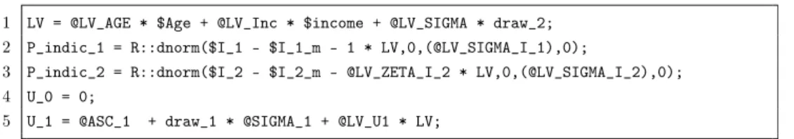
First, in line 1 of Listing 5, we define the structural equation of the latent variable (LV). In lines 2 and 3, we specify the measurement equations. While $I_1 relates to the actual indicator in the data, $I_1_m refers to its pre-computed sample mean. For reasons of
Table 2
Latex model output from a mixed MNL model estimated with mixl Model 1
pf − 0.86∗∗∗
(0.04)
cl − 0.21∗∗∗
(0.02)
loc 1.90∗∗∗
(0.11)
wk 1.38∗∗∗
(0.08)
tod − 7.92∗∗∗
(0.40)
seas − 8.14∗∗∗
(0.37)
sigma_pf 0.18∗∗∗
(0.02)
sigma_cl 0.32∗∗∗
(0.03)
sigma_loc 1.21∗∗∗
(0.12)
sigma_wk 0.30∗
(0.17)
sigma_tod 2.01∗∗∗
(0.24)
sigma_seas 0.89∗∗∗
(0.11)
# estimated parameters 12.00
Number of respondents 361.00
Number of choice observations 4308.00
Number of draws 20.00
LL(null) −5972.16
LL(final) −4108.61
McFadden R2 0.31
AIC 8241.23
AICc 8242.13
BIC 8317.65
∗∗∗p<0.01, ∗∗p<0.05.∗p<0.1.
identification, we set the parameter of the first indicator to 1. For the second indicator, we estimate the parameter @LV_ZETA_I_2.
@LV_SIGMA_I_1 and @LV_SIGMA_I_2 refer to the variances of the error terms of the respective linear regressions. In line 4, the latent variable is included in utility function U_1.
Listing 5. Hybrid choice specification in mixl.
If models include variable definitions with the prefix P_indic_, the model includes hybrid components, and the P_indic_
variables are considered as probability indicators for each observation. P_indic_ should be defined from 1 to k, the number of in- dicators to be used in the model. The pre-compiler detects these automatically and generates the code to include the product of the probability indicators in the log-likelihood (Listing 6).
Listing 6. Calculation of choice probabilities for hybrid choice models in mixl.
One extra column is required in the dataset to enable hybrid choice, namely a ‘count’ column with the total number of observations for the individual making the choice. At model convergence, the estimation output includes both the choice model log-likelihood and the full model log-likelihood.
5.2. Limitations
Mixl is designed to support a core group of models, which in the authors’ experience are used the majority of the time. These include standard MNL, Mixed MNL and hybrid choice models. Furthermore, the design decision was made to only support random heterogeneity across individuals, though not intra-respondent variations. With large datasets and a large amount of draws, even a relatively small number of intra-respondent draws massively increases the memory required. Both Apollo and Biogeme support intra- respondent heterogeneity. The second limitation is that mixl currently only supports the logit kernel. As the code is open-source and
Fig. 1. Performance of the inner log-likelihood function over multiple cores.
simply structured, mixl could be extended with additional model types in the future.
5.3. Post processing
The mixl package provides some key post processing functions for working with an estimated model. The estimation results include all the expected components, such as the (robust) co-variance matrix, table of coefficients, standard errors, Hessian matrix, etc. The posterior function calculates the posteriors for models with mixed distributions. Random variables in the model specification are automatically detected (those with an variable name ending by _RND and including draws), and the posterior function returns a labeled matrix of the posteriors for each individual and random variable. This can all be done inside the R language, as the results of the estimation are always returned as either matrices or dataframes. The probabilities function is useful for calculating elasticities and marginal probability effects, since it calculates the probabilities for each alternative and observation given the estimated pa- rameters. Different scenarios can be easily evaluated by changing specific values (e.g. by 1%) of the input dataset. The summary_tex function outputs the model results in latex table syntax.
6. Performance and multicore scalability
With the widespread availability of multi-core machines and computing clusters, parallel scalability is an important consideration.
mixl achieves consistent speedups even on large numbers of cores. Fig. 1 and Table 3 show the performance of the isolated log- likelihood function for different numbers of draws over an increasing number of cores. To demonstrate the speedup, a pooled RP/
SP MMNL model on a large panel dataset with 491 individuals and 17,120 observations is used (Schmid et al., 2019b). The model contains 27 free parameters, 15 linear-additive utility functions related to four different data/experiment types (mode choice RP, mode choice SP, route choice public transport SP and route choice carsharing SP) and 12 random parameters (six for the ASCs and another six for the mode-specific travel times). The utility functions are a simplified version of the ones presented in Schmid (2019), Chapter 4, including all level-of-service attributes without socio-economic effects and accounting for scale effects between the data/experiment types.
Each timing was repeated 50 times to obtain an average. For the 10 draw configuration, communication costs dominate and a maximum speedup of 4.78×is observed. As the number of draws used is increased, so do the benefits of using parallel computing. On 24 processing cores for 10,000 draws, a speedup of 19.3×is observed. It is worth noting that only the utility calculation has been parallelized, and potential performance improvements in other parts of the log-likelihood function is left for future work. The results in Table 3 show a super-linear speedup in the 4 core case. This can be attributed to cache-effects on the processor.
It is worth noting that the speedups obtained in Table 3 will not necessarily be replicated on real problems, but rather show the upper bound of obtainable performance. This is due to Amdahl’s law, which defines how sequential parts of the program limit the potential gains obtainable with parallel computing. Again, larger problem sizes extract better relative performance from more cores.
More complicated utility functions, i.e. with more alternatives or parameters, will also see a benefit from increased parallelism.
6.1. Further example using the grapes dataset
In the following example, the estimation of an MMNL model based on a modified version of the Grapes dataset (Ben-Akiva et al., 2019) is presented.4 Table 4 presents the attribute values in the dataset. All binary attributes were sampled from independent uniform distributions. There are three grape alternatives that participants can choose from, in addition to the possibility of not choosing any of them. Datasets were generated for 1000, 4000, and 16,000 individuals with 8 observations per respondent.
The model specification is shown in Equations (22)–(27). The utility for alternatives 1,2, and 3 is presented in Equation (22). n denotes the individual decision maker and t the choice task. Four random parameters are included, i.e. one for each variable. As can be inferred from Equations (24)–(27), all parameters follow the univariate normal distribution. The opt-out alternative is depicted in Equation (23).
Vj,n,t=βS,V,n·xS,j,n+βC,V,n·xc,j,n,t+βL,V,n·xl,j,n,t+βO,V,n·xo,j,n,t,j∈ {1,…,3} (22)
V4=0 (23)
βS,V∼N(
βS,σ2S) (24)
βC,V∼N(
βC,σ2C) (25)
βL,V∼N(
βL,σ2L) (26)
βO,V∼N(
βO,σ2O) (27)
Table 3
Speedup over multiple cores for the log-likelihood calculation.
Draws Processors
1 2 4 8 16 24
10 1 1.56 2.81 2.73 3.51 4.78
100 1 1.92 3.83 5.09 6.96 14.76
500 1 1.94 4.04 5.91 9.09 17.40
1000 1 1.95 4.04 6.16 9.60 18.49
5000 1 1.96 4.11 6.28 10.22 19.58
10,000 1 1.97 4.21 6.31 10.25 19.35
Table 4
Grape dataset attributes and levels (Ben-Akiva et al., 2019)s.
Attribute Symbol Levels
Sweetness S Sweet (1) or Tart (0)
Crispness C Crisp (1) or Soft (0)
Size L Large (1) or Small (0)
Organic O Organic (1) or Non-organic (0)
Table 5
Parameters of the Grapes choice model.
Parameter Mean Standard Deviation
B_S 1.00 0.40
B_C 0.90 0.30
B_L 2.50 1.00
B_O 1.50 0.50
Table 6
mixl performance on a large dataset of 128,000 choice observations. Runtime in hh:mm:ss, speedup in brackets.
Draws Processors
1 2 4 8 12 16 24
1 00:00:48 00:00:18 00:00:15 00:00:12 00:00:20 00:00:17 00:00:09
(2.55) (3.06) (3.83) (2.31) (2.79) (4.96)
100 00:20:11 00:10:25 00:06:25 00:03:56 00:03:02 00:02:54 00:02:21
(1.94) (3.14) (5.13) (6.63) (6.95) (8.58)
500 01:54:33 01:02:51 00:32:53 00:21:00 00:13:29 00:15:00 00:09:47
(1.82) (3.48) (5.46) (8.49) (7.64) (11.7)
1000 04:07:52 02:14:21 01:12:57 00:50:42 00:37:46 00:24:03 00:16:10
(1.84) (3.4) (4.89) (6.56) (10.3) (15.32)
5000 18:39:44 09:57:14 05:36:15 03:17:41 02:31:20 01:44:46 01:26:45
(1.87) (3.33) (5.66) (7.4) (10.69) (12.91)
10,000 60:16:29 35:00:28 17:58:11 10:33:33 08:57:10 06:38:54 05:27:31
(1.72) (3.35) (5.71) (6.73) (9.07) (11.04)
Table 7
Speedup relative to mixl by number of processors (higher values are faster).
Program Processors
1 2 4 8 12 16 24
Mixl 1.1.3 1.00 1.00 1.00 1.00 1.00 1.00 1.00
Apollo 0.2.0 0.87 0.73 0.76 0.51 0.50 0.52 0.36
Biogeme 3.2.5 2.16 1.66 1.50 1.35 1.34 1.30 1.08
The true underlying parameters are reported in Table 5. The model is specified in mixl syntax in Listing 7.
Listing 7. MMNL model using the Grapes dataset.
The estimation runtime of an MMNL model in mixl is presented in Table 6. Using 24 cores reduces the execution time by nearly 90%
with 10,000 draws. Furthermore, the speedup is almost linear, implying that further reductions in execution time are possible if more cores are used.
7. Comparisons to other open-source software
The performance of mixl (v 1.1.3) is compared against Apollo (v 0.2.0) and pandasBiogeme (3.2.5), using the same grapes dataset and model specified in Listing 7 above. The demonstrated difference between the performance of Biogeme, mixl and Apollo is pri- marily due to the inclusion or exclusion of two optimisations: compilation of the loglikelihood function to C++, and the imple- mentation of symbolic derivation. In version 0.2.0 of Apollo, analytical gradients have been implemented, giving a 2×speedup over version 0.1.0 on this model and dataset. Section 2 shows why this is the case. However, its reliance on the R language for the utility functions means that it is still slower than mixl. Biogeme implements both symbolic derivation to generate analytical gradients, and compilation to C++, hence it has the best performance. Table 7 shows the performance of the compared programs with respect to the number of processors used, taking the average of different respondent samples (1000, 4000, 16,000) and numbers of random draws (10, 100, 500, 1000, 5000, 10,000). With more processing cores, mixl is as fast as Biogeme, and up to 3.5×faster than Apollo.
The same performance tests were also run for GMNL, which implements analytical gradients, as Apollo and Biogeme do. On the smallest example (1000 respondents and 1000 draws), GMNL had a similar runtime to mixl. However, on a middle size problem with 16,000 respondents and 1000 draws, the code was still running without result after 72 hours. For comparison, Biogeme, mixl and
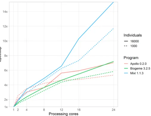
Fig. 3. Speedup over multiple cores for mixl, Apollo and Biogeme on small (n =1000) and large (n =16,000) datasets.
Fig. 4. Comparison of memory usage for mixl, Apollo and Biogeme.
Apollo returned results in 2 hours, 4 hours and 5 hours respectively when using one processing core.
Fig. 2 illustrates how mixl handles larger problems using multicore processing in comparison to Apollo and Biogeme on two program sets, a small one (1000 respondents, 1000 draws), and a medium size one (16,000 respondents, 1000 draws). Although Biogeme is faster when fewer processors are available, the use of openMP for the parallelisation in mixl makes it competitive with Biogeme when more cores are used, especially on larger problems. Similarly, we can see how the R-based parallelisation used by Apollo gives good speedups on larger problems sizes, but doesn’t provide much benefit on more than 4 cores for smaller problems. Fig. 3 shows this from another perspective, with the speedup on the vertical axis. The speedup value is the performance improvement relative to one processing core. For the three programs, we can see how better speedups are achieved on larger problems, as the communication costs become less significant. Also visible is the ability of mixl to better utilise a large number of processing cores - particularly when more than 12 cores are available.
Fig. 4 shows how the memory usage of the different programs compare. A dashed line indicates the predicted memory usage, as the tests were limited by a 200GB memory ceiling. Apollo does take advantage of R vectorization to avoid R’s unoptimized iteration routines, and achieves good results on smaller problems. However, with this technique, the draws must be replicated for each choice task of an individual. The amount of memory required for the duplication means that this approach breaks down for large panel datasets, especially as the number of draws increases, which is required for complex model specifications. The approach used in the mixl package (as in Biogeme) avoids this by accessing the required draws using the ID of the individual. Doing this without R’s performance penalty is possible by using compiled code. For smaller problems the performance is bound by other sequential parts of the program such as the compilation of the likelihood function. Essentially, mixl is not bound by the number of individuals or repeated choices in the dataset, the number of random dimensions or the number of draws used, as long as enough memory is available to store both the data and draws matrix.
8. Conclusion
This paper presents the R package mixl for estimating flexible choice models with a logit kernel. Mixed models and hybrid choice models are supported through a flexible and intuitive syntax. The package has been designed to have an intuitive model specification syntax. For R practitioners considering other model formulations, Apollo is much more flexible, albeit with performance drawbacks and a different syntax. mixl combines compilation to C++code with efficient data structures to allow the estimation of models on large datasets that are not feasible with other R packages, especially if the dataset or number of draws is large. For large problems, parallel computing is an attractive way to gain significant speed increases, and mixl makes it easy for the user to take advantage of this. The paper presents performance indicators on a complex MMNL model estimated on a large dataset with over 128,000 observations, demonstrating speedups in model estimation of over 10×when using 24 cores as opposed to a single core, with no increase in memory usage. The package has also already been used in modelling projects (among them, Schmid et al., 2019a) with thousands of obser- vations and random draws, indicating its robustness and scalability. Future work will aim to integrate the work with other estimation packages such as Apollo and support more model types.
Installing the package
The estimation software is provided as an R package on CRAN https://rdrr.io/cran/mixl/. The code is open-source and shared through Github. A user-guide and documentation are provided with the package.
Author contributions
Joseph Molloy: Conceptualization, Methodology, Software. Writing- Original draft preparation.:Felix Becker: Software, Validation, Writing- Original draft preparation.:Basil Schmid: Conceptualization, Software, Validation.:Kay W. Axhausen: Supervision, Reviewing and Editing.
Declaration of competing interest
The authors have no conflicts of interest to declare. The work was undertaken with the financial support of the SNF and the Deutsche Bahn AG.
Acknowledgements
The authors would like to thank to Stephane Hess, who’s original R script for discrete choice modeling was the inspiration for this R package. We also thank Thomas Schatzmann and the anonymous reviewers for their comments on the paper. The work was undertaken with the financial support of the SNF NRP75 and the Deutsche Bahn AG.
References
ALOGIT, 2016. ALOGIT Software & Analysis Ltd.
Ben-Akiva, M., McFadden, D., Train, K., et al., 2019. Foundations of stated preference elicitation: consumer behavior and choice-based conjoint analysis. Found.
Trends Econom. 10 (1–2), 1–144.
Ben-Akiva, M., McFadden, D., Train, K.E., Walker, J., Bhat, C., Bierlaire, M., Bolduc, D., Boersch-Supan, A., Brownstone, D., Bunch, D.S., Daly, A., de Palma, A., Gopinath, D., Karlstrom, A., Munizaga, M.a., 2002. Hybrid choice models : progress and challenges. Market. Lett. 13 (3), 163–175. ISSN 0923-0645.
Ben-Akiva, M.E., Lerman, S.R., 1987. Discrete Choice Analysis: Theory and Application to Predict Travel Demand. ISBN 0262022176.
Bierlaire, M., 2018. PandasBiogeme: a Short Introduction, Technical Report, Transport and Mobility Laboratory. EPFL, Switzerland.
Chapman, B.M., Massaioli, F., 2005. OpenMP, Parallel Computing 31 (10), 957–1174. ISSN 01678191.
Croissant, Y., 2015. Estimation of Multinomial Logit Models in R: the Mlogit Packages an Introductory Example. Data Management, 01906011.
Czajkowski, M., Budzi´nski, W., 2019. Simulation error in maximum likelihood estimation of discrete choice models. J. Choice Model. 31, 73–85.
Dumont, J., Keller, J., Carpenter, C., 2015. Rsghb: functions for hierarchical bayesian estimation: a flexible approach. R package version 1 (2).
Eddelbuettel, D., Francois, R., 2011. Rcpp: seamless R and C ++integration. J. Stat. Software 40 (8), 1–18. ISSN 15487660.
Greene, W.H., 2002. NLOGIT Reference Guide version 3.0.
Hasan, A., Zhiyu, W., Mahani, A.S., 2014. Fast estimation of multinomial logit models: R package mnlogit. J. Stat. Software 75 (3).
Henningsen, A., Toomet, O., 2011. MaxLik: a package for maximum likelihood estimation in R. Comput. Stat. 26 (3), 443–458, 09434062.
Hess, S., Palma, D., 2019a. Apollo: a flexible, powerful and customisable freeware package for choice model estimation and application. J. Choice Model. 32, 100170.
Hess, S., Palma, D., 2019b. Apollo Version 0.0.9, User Manual, Technical Report.
Hess, S., Train, K.E., Polak, J.W., 2006. On the Use of a Modified Latin Hypercube Sampling (MLHS) Method in the Estimation of a Mixed Logit Model for Vehicle Choice. Transportation Research Part B: Methodological, 01912615.
McFadden, D., 1974. Conditional logit analysis of qualitative choice behavior. In: Zarembka, P. (Ed.), Frontiers in Econometrics, vols. 105–142. Academic Press, 0127761500.
McFadden, D., 1980. Econometric models of probabilistic choice among products. J. Bus. 53 (3), 13–29. ISSN 0012-9682.
McFadden, D., Train, K., 2000. Mixed MNL models for discrete response. J. Appl. Econom. 15 (5), 447–470, 08837252.
Nocedal, J., Wright, S.J., 2000. Numerical Optimization, second ed. Springer. 0387987932.
Sarrias, M., Daziano, R., et al., 2017. Multinomial logit models with continuous and discrete individual heterogeneity in r: the gmnl package. J. Stat. Software 79 (2), 1–46. https://www.jstatsoft.org/article/view/v079i02.
Schmid, B., 2019. Connecting Time-Use, Travel and Shopping Behavior: Results of a Multi-Stage Household Survey. Ph.D. Thesis. IVT, ETH Zurich, Zurich.
Schmid, B., Aschauer, F., Jokubauskaite, S., Peer, S., H¨ossinger, R., Gerike, R., Jara-Diaz, S.R., Axhausen, K.W., 2019a. A pooled RP/SP mode, route and destination choice model to investigate mode and user-type effects in the value of travel time savings. Transport. Res. Pol. Pract. 124, 262–294.
Schmid, B., Axhausen, K.W., 2019. In-store or online shopping of search and experience goods: a Hybrid choice approach. J. Choice Model. 31, 156–180.
Schmid, B., Balac, M., Axhausen, K.W., 2019b. Post-Car World: data collection methods and response behavior in a multi-stage travel survey. Transportation 46 (2), 425–492.
Sobol, I.M., 1967. On the distribution of points in a cube and the approximate evaluation of integrals. USSR Comput. Math. Math. Phys. 7 (4), 86–112.
Train, K.E., 2009. Discrete Choice Methods with Simulation, 2 Ed. Cambridge university press. 1139480375.
van Cranenburgh, S., Bliemer, M.C., 2019. Information theoretic-based sampling of observations. J. Choice Model. 31, 181–197. ISSN 1755-5345.
Walker, J., Ben-Akiva, M., 2001. Extensions of the Random Utility Model, Technical Report. MIT.
Witzgall, C., Fletcher, R., 1989. Practical Methods of Optimization. Mathematics of Computation, 00255718.
Zeileis, A., 2006. Object-oriented computation of sandwich estimators. J. Stat. Software 16 (9), 1–16.
Zeileis, A., K¨oll, S., Graham, N., 2020. Various versatile variances: an object-oriented implementation of clustered covariances in R. J. Stat. Software 95 (1), 1–36.