Abiotic and biotic determinants of height growth of Picea abies regeneration in small forest gaps in the Swiss Alps

(1)

Research Collection

Journal Article

Abiotic and biotic determinants of height growth of Picea abies regeneration in small forest gaps in the Swiss Alps

Author(s):

Schmid, Ueli; Bigler, Christof; Frehner, Monika; Bugmann, Harald Publication Date:

2021-06-15 Permanent Link:

https://doi.org/10.3929/ethz-b-000475538

Originally published in:

Forest Ecology and Management 490, http://doi.org/10.1016/j.foreco.2021.119076

Rights / License:

Creative Commons Attribution 4.0 International

This page was generated automatically upon download from the ETH Zurich Research Collection. For more

information please consult the Terms of use.

(2)

Forest Ecology and Management 490 (2021) 119076

Available online 19 March 2021

Abiotic and biotic determinants of height growth of Picea abies regeneration in small forest gaps in the Swiss Alps

Ueli Schmid

^a^,^*

, Christof Bigler

^a

, Monika Frehner

^b

, Harald Bugmann

^a

aETH Zürich, Department of Environmental Systems Science, Forest Ecology, Universit¨atstrasse 16, CH-8092 Zürich, Switzerland

bETH Zürich, Department of Environmental Systems Science, Forest Management and Silviculture, Universit¨atstrasse 16, CH-8092 Zürich, Switzerland

A R T I C L E I N F O Keywords:

Mountain forest ecology European Alps Norway spruce Forest regeneration Regeneration height

A B S T R A C T

In managed mountain forests, height growth of Norway spruce (Picea abies (L.) Karst) regeneration is a decisive factor for the gap-filling process, especially when the silvicultural goal is to provide continuous protection against natural hazards such as snow avalanches or rockfall. For the planning of management interventions, robust predictions on height growth of regeneration at the scale of forest gaps are thus needed. However, there is a lack of such data for trees of intermediate sizes, and existing studies fail to cover large environmental gradients.

The goal of our study is to identify the key factors that influence height growth of Norway spruce regeneration in small gaps of spruce-dominated forests in the Swiss Alps. Furthermore, we assess whether there are site-specific differences of height growth or whether it follows a similar pattern along a large gradient of temperature (i.e., along elevation) and of water and nutrient availability (i.e., among different phytosociological site types) within the upper montane and subalpine vegetation belts. On 124 plots, >2^′000 observations of annual height in- crements of Norway spruce regeneration (10 cm tree height to 12 cm stem diameter) in gaps were collected.

Using linear mixed effects models and cross-validation for model selection, we identified the best variable combinations to predict annual height growth. Consistently across the entire gradient, the most important factors were 1) the positive effect of tree size, 2) the negative effect of competition by the surrounding stand, and 3) local topography. We found site-specific differences in height growth patterns such as gap size and therefore direct radiation being the most important competition measure in subalpine sites, as opposed to diffuse radiation in high montane sites. However, the pooled model for the entire environmental gradient allowed for predictions of regeneration height growth with similar explanatory power as the more specific models while containing comparable effect sizes. Furthermore, competition can be equally well expressed by metrics based on basal area measurements as by metrics derived from hemispherical photography. Based on these relatively simple models, accurate and robust predictions of the development of Norway spruce regeneration in gaps of managed mountain forests are possible.

1. Introduction

Regeneration, growth, and mortality of trees are core processes that shape long-term forest dynamics. A thorough quantitative understanding of the effects of biotic and abiotic environmental factors on these processes is key for assessing and predicting stand and landscape dynamics. Under harsh conditions, such as at high elevations and high latitudes, these complex processes happen particularly slowly because of strong environmental limitations (Ott et al., 1997). In Europe, this is often the case in forests naturally dominated by Norway spruce (Picea

abies (L.) Karst), a widespread species in mountain ranges and in Scan- dinavia (EUFORGEN, 2009). In the Swiss Alps, Norway spruce is by far the most abundant tree species (Br¨andli et al., 2020) and it is the dominant or co-dominant species in the natural canopy composition on most site types at higher elevations, except on sites with extreme conditions regarding soil moisture, acidity, or constant snow or rock movements (Frehner et al., 2005a).

Growth of Norway spruce has been studied extensively since the beginnings of silvicultural research, e.g. for deriving yield tables (Baur, 1877; Schwappach, 1890). In the last few decades, research has

* Corresponding author at: ETH Zürich, Department of Environmental Systems Science, Institute of Terrestrial Ecosystems, Universit¨atstrasse 16, CH-8092 Zürich, Switzerland.

E-mail address: ueli.schmid@usys.ethz.ch (U. Schmid).

Contents lists available at ScienceDirect

Forest Ecology and Management

journal homepage: www.elsevier.com/locate/foreco

https://doi.org/10.1016/j.foreco.2021.119076

Received 16 October 2020; Received in revised form 25 January 2021; Accepted 15 February 2021

(3)

Forest Ecology and Management 490 (2021) 119076 increasingly focused on mortality of Norway spruce (Bigler and Bug-

mann, 2003; Cailleret et al., 2017; Hülsmann et al., 2018; Monserud and Sterba, 1999). More recently, regeneration of Norway spruce has received increasing attention as well, for example in the context of large disturbances (Macek et al., 2017; Zeppenfeld et al., 2015), browsing by ungulates (Bernard et al., 2017; Kupferschmid et al., 2019; Pröll et al., 2015), and forest management (Downey et al., 2018; Eerikäinen et al., 2014; Hökkä and Mäkelä, 2014; Streit et al., 2009).

In managed mountain forests of the Alps, the promotion of the height growth of regeneration is crucial because large areas of these forests protect human infrastructure from gravitational hazards such as snow avalanches, rockfall, or landslides (Brang, 2001). To ensure continuous protection, foresters commonly facilitate natural regeneration by opening relatively small canopy gaps (Brang et al., 2006), which will eventually be filled by the most vital trees among the regeneration. In the Swiss Alps, planted regeneration plays virtually no role in this management system (Br¨andli et al., 2020). Once these young trees exceed a certain height, they have a protective function against, for example, snow avalanche hazard (Frehner et al., 2005a). Thus, knowl- edge on the factors determining juvenile height growth and therefore the speed of the gap-filling process is pivotal for mountain forest management.

To identify the factors driving height growth of Norway spruce regeneration, most studies have relied either on data from large-scale forest inventories or local field surveys. On the one hand, inventory data can be used for modelling ingrowth of trees larger than a certain diameter threshold (e.g., 12 cm diameter at breast height (DBH) in the Swiss National Forest Inventory; Br¨andli, 2010a). For example, Zell et al.

(2019) showed that the number and diameter of Norway spruce ingrowth in Switzerland can be modelled as a function of stand conditions (developmental stage, basal area, and stand density) and climatic variables (temperature and precipitation). On the other hand, smaller- scale studies on the height growth of Norway spruce regeneration have usually focused on trees from a few centimeters up to 2–4 m in height. In such studies, biotic and abiotic factors found to influence height growth typically include tree-specific variables (e.g., height of the target tree), the substrate or microsite, competing ground vegetation, occurrence of snow mold, the extent of browsing by ungulates, direct and diffuse radiation, slope and aspect, and temperature and water availability during the current and the previous growing season (Cun- ningham et al., 2006; Drobyshev and Nihlgard, 2000; Frehner, 2002;

Hokk¨ ä and Mäkelä, 2014; Kathke and Bruelheide, 2010; Kupferschmid and Bugmann, 2005; Ryter, 2014).

There is, however, a lack of data on the performance of Norway spruce regeneration in the intermediate size classes, i.e. between the surveys on smaller trees and trees measured in forest inventory cam- paigns. Furthermore, most empirical studies on small trees were conducted within relatively small geographical and topographical extents, and only few studies cover a considerable environmental gradient (e.g., Cunningham et al., 2006). This makes it difficult to assess growth patterns of regeneration across a wide range of tree heights and environmental conditions, which would be necessary for a generalized understanding of these processes. To fill these research gaps, we per- formed an extensive field campaign assessing the height growth of Norway spruce regeneration ranging from 10 cm in height up to 12 cm in DBH across a large environmental gradient in the Swiss Alps. Specif- ically, we aimed to answer the following research questions:

(1) What are the key factors influencing height growth of Norway spruce regeneration in small gaps: tree-specific variables (e.g., tree height), the surrounding stand (e.g., competition), climate (e.g., temperature and drought), or topography, respectively?

What is the relative importance of these factors for shaping height growth of Norway spruce?

(2) Are there site- and elevation-specific differences among the main drivers of height growth of Norway spruce? How well can height

growth be predicted across a large environmental gradient with a single model?

2. Material and methods 2.1. Study site selection

Study sites were selected within the most abundant site types, i.e.

phytosociological associations, of the high montane (HM) and subalpine (SA) elevational zones (sensu Frehner et al., 2005a) of the Swiss Alps.

Forests of the high montane zone are usually dominated by Picea abies and Abies alba Mill., are characterized by a homogeneous horizontal structure, and occur at elevations between 1^′300 m (sometimes even down to 600 m) and 1^′700 m a.s.l., while subalpine forests are dominated by Picea abies alone, show a distinct clustered horizontal structure, and occur at elevations between 1^′500 m and 2^′000 m a.s.l. (ARGE, 2020; Frehner et al., 2005a). We chose the site types for our study based on data from the NaiS-LFI Project (ARGE, 2020), in which a site type was assigned to each sample plot of the Swiss National Forest Inventory NFI (Br¨andli, 2010a; WSL, 2018a). For a detailed description of the selection process, see Appendix A.1 in the supplementary material. The selected site types were grouped into four strata (HM1, HM2, SA1, SA2) according to similarities in their regeneration ecology, soil acidity and moisture (Table 1). The site types included in the high montane and subalpine strata account for 52% and 47% of all sample plots of the NFI in the corresponding elevational zone, respectively. Using forest maps provided by the regional authorities, we identified areas that contained large patches of the corresponding site types and covered a climatic gradient (i.e., different ecoregions sensu Frehner et al., 2005a) throughout the Swiss Alps and were thus suitable for field sampling.

The exact location of the study plots (Fig. 1) was determined in situ based on the following criteria: (1) Each circular plot had to consist of a central forest gap (no trees with DBH >12 cm) and the surrounding stand. (2) The gap had to contain viable natural spruce regeneration (DBH <12 cm) in its center and have a radius of at least 4 m in HM and 3.5 m in SA, measured from the plot center to the stem base of the closest tree of the surrounding stand (i.e., the “extended gap“ sensu Runkle, 1982). (3) The plot must not have been affected by major natural or anthropogenic disturbances over the previous decade (e.g., no fresh stumps, broken or fallen stems). The minimum gap radii were defined based on the crown projection areas of spruce and silver fir (Pretzsch, 2014), which decrease with elevation. Correspondingly, the plot radii were set to 17.6 m and 15.4 m in HM and SA plots, respectively.

We selected 124 plots (Table 1) that were distributed equally over the four strata. They were located mainly in the eastern part of the northern Pre-Alps, the northern intermediate Alps, the continental central Alps, and the southern intermediate Alps (Fig. 1). The elevation of the plots varied between 1^′048 and 2^′018 m a.s.l. Annual mean temperatures ranged from 0.7 to 8.9 ^◦C and annual precipitation sums from 670 to 2^′853 mm in the years 2010 to 2018 (Remund et al., 2016).

2.2. Sampling design

Among the Norway spruce regeneration (DBH <12 cm) in each gap, the tallest, most vigorous and locally dominating trees were selected for measurements. Depending on the spatial arrangement of the regeneration clusters within the gap, this resulted in one to seven trees per gap and 324 trees in total (Table 1). Their current height was recorded, as well as their height at the end of the previous growing seasons as far back as this could be determined clearly by the position of the bud scars and whorls. The series of retrospectively measured tree heights had to be continuous and went back no further than the year 2010. Overall, we recorded 2^′305 observations of annual height growth ranging between 1 and 63 cm and tree heights (before growth) from 6 to 873 cm (Table 1).

Data collection took place in summer and autumn of 2018 and 2019.

Heights were measured using a ruler for trees up to ca. 5 m in height U. Schmid et al.

(4)

and a Vertex IV (Hagl¨of, Sweden) for taller trees (mean of three repeated measurements, rounded to the nearest cm). We registered years in which the main shoot had probably been browsed and was replaced by a side shoot (so-called flagging; cf. Kupferschmid et al., 2014) as well as other damages to the target trees such as wounds on the stem or snow mold infection of the foliage. The terrain form within a radius of 1 m of each target tree, henceforth referred to as microtopography, was classified as even, mound, or depression.

Two approaches were chosen to characterize competition between the target trees and the surrounding stand. First, we measured the DBH and the relative position to the plot center of each living tree and snag with a DBH >4 cm between the minimum gap radius and the plot radius. The relative position was determined by the horizontal distance to the plot center and the angle, measured with a Vertex and a magnetic compass, respectively. Second, light availability within the gap was assessed using hemispherical photographs (Schleppi et al., 2007). A Canon EOS 70D camera was positioned on a tripod either in the plot center or, if impeded by larger regeneration, half the minimal gap radius to the south of it, and the lens (Sigma 4.5 mm F2.8 EX DC HSM Circular Fisheye) was fixed at 1.5 m above ground. We took seven photos with differing exposures to assure ideal picture quality for the analysis.

We recorded the following variables to characterize the abiotic conditions of each plot: (1) coordinates of the plot center, which were later used to derive interpolated climate data; (2) elevation; (3) aspect and slope angle (mean of two measurements, up- and downhill from plot center); (4) macrotopography, i.e. terrain form of the entire plot, again

classified as even, mound, or depression. Additionally, we obtained historical daily temperature and precipitation data for the years 2010 to 2018 for each specific plot location from an interpolated data set (Remund et al., 2016).

2.3. Data preparation

We processed all field measurements to obtain response, explanatory, and grouping variables for the statistical analysis (Table 2). Unless stated otherwise, all calculations were conducted in the R statistics software (R Core Team, 2020). Net annual height growth per calendar year (response variable HGr) was calculated as the difference in measured tree heights at the end of each growing season (explanatory variable TrH). Observations of height growth in 2018 were included in the analysis if the tree had been measured in September 2018 or later since height growth can be assumed to be completed by September (Dobbertin and Giuggiola, 2006; Konˆopka et al., 2014; Ryter, 2014).

Observations of annual height growth in which the height increment was likely realized by a lateral shoot due to browsing (flagging, cf.

above) accounted for ca. 5% of all cases and were included in the analysis.

To quantify competition, i.e. the effect of the surrounding stand on the regeneration, a total of eight competition indices were computed.

Since only plots without clear signs of disturbance during the observation period of no more than 8 years were included in this study, all es- timates of the competition indices were assumed to be constant over this Table 1

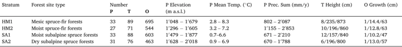
Number of plots (P), trees (T), and observations of annual height growth (O) per stratum. Minimum and maximum values of plot elevation. Minimum and maximum of annual mean temperature and annual precipitation sum at plot locations in the years 2010–2018. Minimum/mean/maximum of tree height and annual height growth.

Stratum Forest site type Number P Elevation

(m a.s.l.) P Mean Temp. (^◦C) P Prec. Sum (mm/y) T Height (cm) O Growth (cm)

P T O

HM1 Mesic spruce-fir forests 33 89 695 1^′048 − 1^′679 2.8 – 8.3 802 – 2^′087 8/235/873 1/14.4/63

HM2 Moist spruce-fir forests 27 71 544 1^′296 − 1^′605 3.2 – 7.2 1^′155 – 2^′853 10/196/860 1/12.8/63

SA1 Moist subalpine spruce forests 33 88 603 1^′479 − 1^′877 0.7–6.6 671 – 2^′210 12/157/840 1/10.2/47

SA2 Dry subalpine spruce forests 31 76 463 1^′628 − 2^′018 0.9 – 6.9 670 – 1^′788 6/196/800 1/13.0/57

Fig. 1.Distribution of the 124 plots across the Swiss Alps and the ecoregions of Switzerland according to NaiS (Frehner et al., 2005a). Plots are locally clustered and therefore often overlayed at this scale. Base map of Switzerland: swisstopo (2020).

(5)

Forest Ecology and Management 490 (2021) 119076 time.

First, we calculated five basal area-related indices based on the DBH and position of the trees: total basal area per ha (BA, Eq. (1a)); basal area weighted by the cardinal position of the tree, prioritizing trees south of the plot center using maximum weights (w_max) of 4 (BA_wS04) and 10 (BAwS10) respectively (Eq. (1b)); and basal area weighted by the distance of the tree to the plot center, prioritizing trees closer to the gap edge again using maximum weights of 4 (BAwD04) and 10 (BAwD10), respectively (Eq. (1c)).

BA=A⁻¹∑_n

i=1bai (1a)

BAwSwmax=A⁻¹∑_n

i=1bai* [(

1− |180− ai| 180

)

*(wmax− 1) +1 ]

(1b)

BAwDwmax=A⁻¹∑_n

i=1bai*

[dmax− di

dmax− dmin*(wmax− 1) +1 ]

(1c) where A is the plot area (ha), bai is the basal area of tree i (m²), n is the number of trees within the plot, a_iis the azimuth of the tree (^◦from north), wmax is the maximum weight assigned, dmax is the plot radius (m), di is the distance of the tree to the plot center (m) and dmin is the minimum gap radius (m). During early stages of the analysis, we tested wmax

values between 2 and 10 and decided to use 4 and 10 based on the performance of the resulting indices as predictors for height growth.

Only living trees entered the calculations.

Second, based on the hemispherical photographs and the plot coordinates, we calculated three light-based indices: Diffuse Light Index (DLI), Beam Light Index (BLI), and Global Light Index (GLI). The indices are defined as the proportion of radiation reaching the gap center compared to a hypothetical spot on flat ground and without surrounding vegetation, expressed as a percentage (Zellweger et al., 2019). For the DLI and BLI, only diffuse and direct radiation are considered, respectively, while both types of radiation are considered in the GLI. The indices were calculated using the software Hemisfer (Schleppi et al., 2007) for the months June and July, a period that is known to reflect light conditions during the whole growing season well (Frehner, 2002).

The historical temperature and precipitation records were used to characterize conditions during the year of height growth (period of height growth only) and the preceding year of bud formation (complete growing season to include the late phase of reserve building). Temper- ature regimes were quantified with degree-day sums, calculated for each plot using the historical daily minimum and maximum temperature records and a threshold temperature of 5.5 ^◦C (Tranquillini, 1979). For the year of height growth, the daily degree-day sum from January to August (DD_curr) was used, for the previous year, the degree-day sum from January to December (DDprev). To quantify water availability, the Standard Precipitation and Evapotranspiration Index (SPEI; Vicente- Serrano et al., 2010) was used. It was calculated for each plot based on the historical monthly mean temperature and precipitation records as well as the latitude of the plot, using the R-package SPEI (Beguería and Vicente-Serrano, 2017; Version 1.7). For the year of height growth, the SPEI from April to August (SPEIcurr) was used, for the previous year, the SPEI from April to October (SPEIprev). As precipitation can be expected to fall as snow from November to March at the elevations of our plots, these months were not included in the SPEI calculation.

From the measured aspect and slope angles, we calculated a single variable characterizing the topographical position of a plot (SloAsp).

This variable served as an estimate of the relative water retention potential and is based on a concept used in Bugmann (1994). Calculated according to Eq. (2), based on Bennie et al. (2008), SloAsp takes on minimal values on steep southern slopes, a value of 0 on horizontal sites and maximal values on steep northern slopes:

SloAsp= [cos(slope) +sin(slope)*cos(aspect) ] − 1 (2) where slope is the slope angle of the plot (rad) and aspect is the azimuth Table 2 Description of the variables and their grouping used to build the conceptual and statistical models. Type Group§Variable Explanation Unit/Levels Source/Remarks Response variable HGr Annual height growth cm log-transformed Explanatory variables Tree height TrH Tree height before growth cm log-transformed Competition* BA Basal area of surrounding stand m2/ha Eq. (1a) BAwS04 BA index, weighted by cardinal direction – Eq. (1b), wmax =4 BAwS10 BA index, weighted by cardinal direction – Eq. (1b), wmax =10 BAwD04 BA index, weighted by distance from plot center – Eq. (1c), wmax =4 BAwD10 BA index, weighted by distance from plot center – Eq. (1c), wmax =10 DLI Diffuse Light Index for June and July % Hemisfer BLI Beam Light Index for June and July % Hemisfer GLI Global Light Index for June and July % Hemisfer Temperature** DDcurr Degree-day sum from Jan. to Aug. of the current year ◦*d Daily temperature records DDprev Degree-day sum from Jan. to Dec. of the previous year ◦*d Daily temperature records

Water availability

** SPEIcurr SPEI from Apr. to Aug. of the current year – Monthly temperature and precipitation records SPEIprev SPEI from Apr. to Oct. of the previous year – Monthly temperature and precipitation records Slope/Aspect SloAsp Relative water retention potential – Eq. (2) Topography* TopoTree Microtopography, i.e. terrain form around target tree even†, mound, depression Radius =1 m TopoPlot Macrotopography, i.e. terrain form of sample plot even†, mound, depression Radius =15 m Grouping variables TreeID ID of target tree – Used for random intercept Year Calendar year of height growth observation – Used for temporal autocorrelation §Groups were used for the identification of the conceptual models, cf. text. *Only one variable per group included in models. **One or both variables per group included in models. †Reference level.

U. Schmid et al.

(6)

of the plot (rad from north).

2.4. Statistical analysis

To analyze the effects of the explanatory variables (Table 2) on annual height growth, linear mixed effects models (LMM) of the following form were calculated:

HGrit=β0+∑ⁿ

j=1

βj×Vj,it+bi+εit (3)

where HGrit is the height growth of tree i in year t, β_jis the coefficient of the fixed effect of variable Vj, bi is the random intercept of tree i with bi∼ N(

0,σ²_b⁾, and ε_itis the residual error of tree i in year t with ε_it∼ N(0,σ²). The fixed effects Vj of the models were determined in a two- step process. First, 17 conceptual models with variable groups as fixed effects were defined (“group” in Table 2, second column). The simplest of these models included only tree height, whereas more comprehensive models consisted of all possible combinations of at least two variable groups, with tree height and competition included in each of them as they were deemed important a priori. Second, multiple statistical models were formulated based on each conceptual model by substituting the variable groups with their corresponding explanatory variables (“variable” in Table 2, third column). From the competition and topography groups (Table 2), only one variable was used in each model, whereas from the temperature and water availability groups, one or both variables were used. This resulted in a total of 769 statistical models. Annual height growth (HGr) and tree height (TrH) were log-transformed to linearize their relationship. All models included random intercepts for each tree (b_i). An autoregressive parameter φ of order 1 (AR-1, Eq. (4)) was added to the models to account for temporal autocorrelation of HGrit

(Pinheiro and Bates, 2000):

εt=φ×εt−1+η_t (4)

where ε_t-1is the residual error in the previous year and η_tis a noise term with zero mean. Model parameters were estimated using the R-package nlme (Pinheiro et al., 2020; Version 3.1) and the restricted maximum likelihood (REML) method.

The predictive power of each model was assessed with the root mean square error (RMSE) of the residuals (back-transformed from the log- scale to cm) obtained through k-fold cross validation. Per fold, all observations of one tree were used as test data (Pinheiro and Bates, 2000) and predictions were made using only the fixed effects. The models were evaluated on seven data sets: each of the four strata separately (HM1, HM2, SA1, and SA2) and the pooled data of one or both elevation zones (HM, SA, and HMSA; hereafter also referred to as strata). Per stratum, the model with the smallest RMSE was selected for further analysis. For each of these seven models, we calculated the mean error (i.e., residuals in cm) based on the fixed effects (ME0) as well as based on the fixed and random effects (ME1). Furthermore, we calculated the marginal and conditional coefficient of determination (R²m and R²c) with the R- package MuMIn (Barto´n, 2019; Version 1.43). Additional model diagnostics (not shown) consisted of variance inflation factors (Fox and Monette, 1992), standard residual plots, plots of residuals vs. each explanatory variable, and normal Q-Q plots of random intercepts. None of the model diagnostics revealed any violations of model assumptions.

We omitted the observations of one plot consisting of a single tree in HM2 (numbers in Table 1 represent the data effectively used in the calculations). Within this stratum, it was the only tree with the value of TopoTree being depression. Therefore, the height growth of this tree could not have been predicted while cross-validating the 256 statistical models containing the variable Topo_Tree. Consequently, the data of this tree was also omitted in the pooled data sets HM and HMSA.

The effect size of the explanatory variables was derived from the predictions of annual height growth using the estimated fixed-effect

parameters (Forrester et al., 2017). For each of the seven final models, we computed the change in predicted values when changing one of the explanatory variables by one standard deviation while keeping the other explanatory variables constant at their mean within its corresponding data set. The effect sizes were expressed as a percent change in predicted height growth compared to predictions where all explanatory variables were kept at their corresponding mean value.

The same analysis was repeated with models including a second, higher level grouping variable for the random intercepts. For this pur- pose, all plots were aggregated into 28 field sites, geographical clusters on the scale of whole slopes. The random effects for each tree were then nested within the field sites. These results are presented in Appendix A.3 in the supplementary material.

3. Results

3.1. Model descriptions

Out of the 769 LMMs calculated for each stratum, we selected the model for further analysis that predicted annual height growth of spruce regeneration (HGr) with the highest accuracy, i.e. the model with the lowest RMSE in cross-validation. The fixed effects structure of these seven models as well as the corresponding statistics are presented in Table 3.

The pooled model (HMSA) that most accurately predicted the height growth data of spruce regeneration from both elevational zones contained explanatory variables from five out of six variable groups: tree height, competition, temperature, water availability, and topography. All six predictors were highly significant according to t- and F-tests (p-values <

0.005). From the competition variables, the basal area-based index BA_wD10was chosen, which correlated negatively with height growth.

Temperature during the growing season (DDcurr) as well as water availability during the current (SPEIcurr) and the previous growing season (SPEI_prev) showed a positive relationship with height growth. On even plots (TopoPlot), height growth was significantly larger than in depressions.

The SA model that best predicted height growth in the subalpine elevational zone contained six explanatory variables from all six variable groups. The following four fixed effects were highly significant (p- values <0.001): positive effects of TrH and SPEIcurr and a negative effect of BAwD10 (as in HMSA) as well as the microtopography (TopoTree). Trees on mounds grew significantly less than trees on even ground. Albeit not statistically significant, DDprev and SloAsp were also included as fixed effects in the model.

The two models for each of the separate subalpine strata, SA1 and SA2, also contained the competition variable BAwD10 and the topography variable Topo_Tree(microtopography). In SA1, height growth increased significantly with water availability in the current and the previous year (SPEIcurr and SPEIprev), but temperature had no effect. In SA2, however, water availability did not influence height growth, whereas the temperature in the current growing season (DDcurr) had a negative influence.

Additionally, microtopography (TopoTree) was only marginally significant in SA2.

Within the high montane elevational zone (HM), height growth of spruce regeneration was predicted best by a model with seven significant fixed effects (p-values <0.02), representing all six variable groups.

Unlike in HMSA and the three subalpine strata, the Diffuse Light Index (DLI) was selected to represent competition by the surrounding stand, correlating positively with height growth. The two weather-related variables of the current growing season (DD_currand SPEI_curr) as well as SPEIprev had a positive effect on height growth. The positive relationship between height growth and SloAsp indicates that trees on north-facing slopes tended to grow more than trees on south-facing slopes. As in HMSA, the macrotopography (TopoPlot) was included in the model.

The two separate models for HM1 and HM2 contained similar effects of DDcurr, SPEIcurr, SPEIprev, and TopoPlot as the HM model. However,

(7)

ForestEcologyandManagement490(2021)119076

6

Table 3

Best-performing models (Eq. (3) and Table 2) per stratum according to cross-validation explaining log-transformed height growth including summary statistics. Per group of explanatory variables, the variables included as fixed effects, their respective coefficients, and p-values from t-tests are listed.

Explanatory variable groups Model statistics^a

Stratum Intercept Tree height^b Competition Temperature Water availability Slope/aspect Topography^c φ σ_b σ _RMSE _ME₀ _ME₁ _R²_m _R²_c

HMSA Intercept TrH BAwD10 DDcurr SPEIcurr SPEIprev TopoPlot mound depr. 0.25 0.36 0.43 7.59 −1.85 −1.11 0.57 0.75

Coefficient −0.200 0.603 −0.004 4E-04 0.087 0.067 − 0.028 − 0.172

SE^d 0.164 0.023 4E-04 1E-04 0.013 0.012 0.058 0.056

p-value 0.222 <0.001 <0.001 <0.001 <0.001 <0.001 0.005 0.632 0.002

SA Intercept TrH BAwD10 DDprev SPEIcurr SloAsp TopoTree mound depr. 0.30 0.35 0.46 7.14 −1.61 −1.14 0.53 0.70

Coefficient 0.677 0.553 −0.004 − 2E-04 0.066 −0.058 − 0.276 0.095

SE^d 0.266 0.035 0.001 1E-04 0.016 0.109 0.076 0.155

p-value 0.011 <0.001 <0.001 0.113 <0.001 0.598 <0.001 <0.001 0.539

SA1 Intercept TrH BAwD10 SPEIcurr SPEIprev TopoTree mound depr. 0.31 0.28 0.47 6.15 −1.33 −1.08 0.50 0.63

Coefficient 1.120 0.457 −0.005 0.064 0.082 − 0.380 − 0.069

SE^d 0.364 0.053 0.001 0.022 0.025 0.088 0.275

p-value 0.002 <0.001 <0.001 0.003 0.001 <0.001 <0.001 0.804

SA2 Intercept TrH BAwD10 DDcurr TopoTree mound depr. 0.26 0.39 0.43 7.49 −1.85 −1.12 0.58 0.77

Coefficient −0.017 0.691 −0.005 −4E-04 − 0.029 0.399

SE^d 0.325 0.052 0.001 2E-04 0.128 0.197

p-value 0.959 <0.001 <0.001 0.023 0.053 0.822 0.047

HM Intercept TrH DLI DDcurr SPEIcurr SPEIprev SloAsp TopoPlot mound depr. 0.23 0.33 0.41 7.61 −1.97 −1.08 0.65 0.78

Coefficient −2.082 0.664 0.023 0.001 0.099 0.084 0.258 − 0.120 − 0.285

SE^d 0.217 0.029 0.003 1E-04 0.018 0.016 0.108 0.083 0.072

p-value <0.001 <0.001 <0.001 <0.001 <0.001 <0.001 0.018 <0.001 0.152 <0.001

HM1 Intercept TrH DLI DDcurr DDprev SPEIcurr SPEIprev SloAsp TopoPlot mound depr. 0.24 0.28 0.41 7.42 −1.87 −1.16 0.70 0.80

Coefficient −1.443 0.643 0.022 0.001 − 5E-04 0.124 0.060 0.496 − 0.261 − 0.430

SE^d 0.292 0.035 0.004 2E-04 2E-04 0.023 0.023 0.115 0.096 0.095

p-value <0.001 <0.001 <0.001 <0.001 0.005 <0.001 0.008 <0.001 <0.001 0.008 <0.001

HM2 Intercept TrH BAwD10 DDcurr SPEIcurr SPEIprev TopoPlot mound depr. 0.22 0.34 0.42 7.09 −1.61 −0.94 0.64 0.79

Coefficient −0.266 0.631 −0.006 5E-04 0.071 0.084 0.453 − 0.126

SE^d 0.382 0.047 0.001 3E-04 0.033 0.023 0.196 0.106

p-value 0.486 <0.001 <0.001 0.087 0.033 <0.001 0.004 0.024 0.239

aφ: autoregressive parameter; σ_b: standard deviation of random intercept; σ: standard deviation of residuals; RMSE: root-mean-square error (cm) from cross-validation; ME0: Mean error (pred. - obs., cm) with fixed effects only; ME1: Mean error (pred. - obs., cm) with random intercepts; R²m: marginal R-squared; R²c: conditional R-squared.

b log-transformed.

cp-value of the variable as a whole calculated using F-test; p-values of levels 2 and 3 (from t-tests) indicate difference from the reference level, even.

dSE: Standard error of the coefficient estimate.

U. Schmid et al.

(8)

while the HM1 model also contained DLI as the competition variable (positive correlation), BA_wD10was selected in the HM2 model (negative correlation). Furthermore, height growth increased with decreasing DDprev and increasing SloAsp (both effects statistically significant) in HM1, but not in HM2. Trees in plots classified as depressions (Topo_Plot) grew less than trees in even plots in all three high montane strata, while trees on mounds grew less in HM1 and more in HM2 compared to trees on even plots.

3.2. Prediction accuracy

The seven models (Table 3) all had a similar prediction accuracy. The SA1 model was most accurate based on its fixed effect structure, with an RMSE of 6.15 cm and a ME0 of − 1.33 cm. When including the random intercepts of each tree in the predictions, the HM2 model allowed for the least biased predictions, as shown by the ME₁of − 0.94 cm. Considering the range of measured HGr of 1 to 63 cm (Table 1), the values of these three metrics differed little between the seven models. Prediction accuracy did not systematically differ between elevational zones (high montane vs. subalpine) or between strata of single site type groups and of pooled data (e.g., SA1/SA2 vs. SA). All seven models tended to un- derestimate HGr according to the mean errors. This can be attributed primarily to the underestimation of large annual height growth observations.

Based on the variance explained, quantified by R²m for the fixed effects and R²c for the fixed and random effects combined, all models featured very good performance, with the three models of the high montane strata outperforming the models of the subalpine strata and the pooled data HMSA. The three high montane models each explained 78 to 80% of the variance when including the random intercepts, while the subalpine models explained between 63 and 77% and the HMSA model reached 75%. However, no pattern in explanatory power was visible when comparing models for separate site type groups to models based on the pooled data. Models of all seven strata contained temporal autocorrelation (Table 3). The effects were not particularly strong, but significant since the 95% confidence interval of φ did not include zero in any model. Temporal autocorrelation was stronger in the subalpine strata than in the high montane strata.

3.3. Analysis of variable groups

Variables from the variable groups tree height, competition and topography were included in each of the seven models (Table 3). Their effects were highly significant in all but one case and they had the largest mean effect on height growth (Table 4). The most influential variable was TrH. Changing it by plus or minus one standard deviation while keeping all other variables fixed at their mean caused an average change

of 57% in predicted values of HGr across the seven models (Table 4).

While the value of the coefficient of TrH was similar in the three high montane models, it varied more strongly among the subalpine strata (Table 3). Visualizing the effect of TrH on height growth over the whole range of sampled tree heights (Fig. A1) revealed that the difference between SA1 and SA2 (less height growth at a given tree height in SA1) was substantial. This pattern was most pronounced for large tree heights.

The competition variables had the second largest influence on HGr with an average effect size of 27% across the seven models (Table 4). In five out of seven models, the competition of the surrounding stand was characterized by an index based on the basal area of the surrounding stand (BAwD10). Its effect was of similar magnitude in all these strata (Table 3 and Fig. 2). In contrast, a light-based competition index (DLI) was selected in HM and HM1. The effect of DLI was weaker than that of BAwD10 (Fig. 2), but the shape of the effect curve over the whole range of sampled data of both competition indices was similar (Fig. A1).

To further analyze the representation of the competition effect by different indices, we compared the predictive power of additional models. For each stratum and number of variable groups included in the models, we selected the most accurate models according to the RMSE with either a basal area-based or a light-based competition index (Fig. 3). In all strata except for HM, there was a consistent difference in predictive power between models with competition indices based on basal area vs. light. In HMSA, in all three subalpine strata, and in HM2, basal area-based competition indices outperformed light-based indices regardless of the number of variable groups included. In HM1, the opposite pattern was evident, with light-based indices allowing for more accurate models, especially when more than three variable groups were included.

The mean effect size of the topography variables on HGr in the seven models of Table 3, when changing variable levels, amounted to 20%

(Table 4). In HMSA and the three high montane strata, macrotopography (Topo_Plot) was included, with the smallest height growth rates occurring in plots classified as depressions. With the exception of HM2, the largest growth rates were observed on even plots. In the three subalpine strata, microtopography (TopoTree) was included in the models, and trees on mounds grew less than trees on even ground or in depressions.

The four weather-related variables DDcurr, DDprev, SPEIcurr and SPEI-

prev as well as SloAsp had mean effect sizes < 10% and were not consistently part of the seven models of Table 3, and the sign of the response varied.

When using random intercepts for each tree nested within the field sites, the most accurate models per stratum were very similar to those presented above with a single random intercept per tree. The fixed effects had similar coefficients, and their relative importance in terms of mean effect size was identical. Furthermore, the model statistics (RMSE, ME and R²) differed only little. The differences in the model structures considering only significant fixed effects lay in the competition variables (BAwD04 instead of BAwD10 in SA1 and SA2, and GLI instead of DLI in HM) and in the presence or absence of weather-related variables (DDcurr in HMSA, SPEIprev in SA1, and DDprev in HM). The detailed results can be found in Table A1.

4. Discussion

4.1. Key factors determining height growth of Picea abies regeneration Our study covered a wide environmental gradient and we found that tree height always had the largest effect on the height growth of regeneration. There was a positive interaction between tree height and height growth, with the slope being steepest at small tree heights. Such a relationship has previously been shown in studies under widely different conditions such as under closed canopy, in gaps as well as under open conditions, among others in the montane and subalpine zones of the Table 4

Effect sizes of variables or variable groups in the models of Table 3, expressed as the absolute percent change of predicted HGr when changing the respective variable by plus and minus one standard deviation, or one level in case of the topography variables, and keeping all other variables at their mean. The variables are ordered by descending mean effect size.

Variable/Variable group n^a Effect size (%)

min. mean max.

TrH 7 30.0 57.4 83.1

Competition 7 18.1 26.8 40.6

Topography 7 2.8 19.9 57.2

SloAsp 3 1.8 8.3 17.1

DDcurr 5 4.5 7.6 12.8

SPEIcurr 6 5.1 7.5 11.8

DDprev 2 3.0 5.5 8.3

SPEIprev 5 4.1 5.5 6.4

aNumber of models out of the seven in Table 3 that include this variable or variable group.

(9)

Forest Ecology and Management 490 (2021) 119076

Swiss Alps (Cunningham et al., 2006; Kupferschmid and Bugmann, 2005), in the montane zone of the German Black Forest (Danescu et al., ˘ 2018) and in the Bavarian Forest (Macek et al., 2017), in southern and northern Finland (Eerikäinen et al., 2014; Hokk¨ ä and Mäkelä, 2014;

Laiho et al., 2014) as well as in the Russian Taiga (Drobyshev and Nihlgard, 2000). It is important to note that most of these studies focused on trees shorter than a few meters. Our findings therefore are notable because they extend the validity of this relationship to larger

trees, up to the early pole stage.

Tree height and height growth of the terminal shoot are only two out of multiple possible variables for characterizing the size and growth of a tree (Cunningham et al., 2006). However, we were able to demonstrate a strong relationship between these two variables, which are much easier to measure than for example total carbon gain and allocation. For this pragmatic reason and due to the importance of tree height and height growth of the regeneration in the gap-filling stage in forests that protect Fig. 2. Predicted changes in HGr in response to changes in each explanatory variable using the fixed effects structure of the models (cf. Table 3). The symbols (circles and triangles) represent the mean predicted values for each stratum. The arrows show the predicted changes in HGr when (1) all variables except those indicated on the x- and y-axes are kept constant at their means for the given stratum and (2) the respective explanatory variable is increased or decreased by one standard deviation (a-g) or its level is changed (h). A solid arrow indicates a highly significant effect (p <0.01), a dotted arrow a moder- ately significant effect (0.01 < p < 0.05). The absence of an arrow indicates either no effect, i.e. the variable is not included in the model, or an insig- nificant effect (p > 0.05). In (b), circles indicate models containing BAwD10 and triangles indicate models containing DLI as the competition variable. In (h), circles indicate models containing macrotopography (TopoPlot) and triangles indicate models containing microtopography (TopoTree) as the topog- raphy variable. The levels of the topography variables on the x-axis are sorted by increasing values of HGr for each model.

U. Schmid et al.

(10)

human infrastructure from natural hazards, for example, we recommend their use in future studies.

In the subalpine zone, the effect of tree height on growth was considerably smaller on moist sites (SA1) than on dry sites (SA2), i.e.

lower growth was found for a given height, especially in larger trees.

There is no clear reason for this pattern, but we surmise that the higher input of direct radiation and therefore warmth on the mostly south- facing dry sites (SA2) outweighs potential growth limitations due to drought at high elevations (K¨orner, 2012). The importance of warmth for the growth of tree regeneration at the subalpine level has been shown repeatedly (Frehner, 2002; Imbeck and Ott, 1987; Ott et al., 1997), although soil properties – and thus drought – were also found to be important at high elevations in the Rocky Mountains (Bugmann, 2001) and, more recently, in the European Alps (Huber et al., 2021). However, we were not able to substantiate this hypothesis based on the empirical patterns comparing either BLI, the light index characterizing direct radiation, or degree-day sums between the two strata.

Competition by the surrounding stand was the second most important factor determining height growth in all models. The number, size, and spatial distribution of the neighboring trees affect a range of resources that are important for the regenerating trees, including direct radiation (warmth), photosynthetically active radiation, access to nu- trients and water, and rooting space. The importance of properties of the surrounding stand on the growth of spruce regeneration has been shown

using a range of proxies characterizing competition, which can be summarized in two broad categories. On the one hand, there are indices based on light measurements, used e.g. by Imbeck and Ott (1987) and Frehner (2002), who found positive linear correlations of the height growth of regeneration with (1) the potential duration of direct sunlight in June and July and (2) the share of open sky, and by Cunningham et al.

(2006), who found a quadratic relationship between Leaf Area Index (LAI) and height growth. On the other hand, there are indices based on forest structural properties, used e.g. by Laiho et al. (2014) and Eer- ik¨ainen et al. (2014), who found a negative linear correlation between local stand basal area and height growth. We tested both approaches and found them to have high predictive power, as evident from the strong negative effect of basal area and the positive effect of light indices, as evaluated below.

In our models, the most influential competition indices in the subalpine zone and for the pooled data were BAwD10, i.e. local stand basal area weighted by the proximity to the regeneration, and in the high montane zone DLI, i.e. the Diffuse Light Index. BAwD10 is closely asso- ciated with gap size, and therefore, these findings are in line with previous work highlighting the importance of direct radiation and therefore warmth as a pivotal factor for regeneration in the subalpine zone, while diffuse radiation is more important for regeneration in high montane forests (Frehner, 2002; Imbeck and Ott, 1987; Lüscher, 1989). Two studies that explicitly compared competition indices as predictors for Fig. 3.RMSE of the most accurate models for predicting height growth depending on the number of variable groups included and on whether the competition index is based on basal area of the surrounding stand (filled symbols) or on measurements of light availability (empty symbols).

(11)

Forest Ecology and Management 490 (2021) 119076 growth of spruce regeneration (Chrimes and Nilson, 2005; D˘anescu

et al., 2018) found light-based indices (canopy openness and crown projection area, respectively) to be more closely related to height growth than basal area of the surrounding stand. In contrast, we found that a basal area-based competition index yielded the most accurate predictions across both elevational zones, which is much easier to deter- mine in the field than light-based indices via hemispheric photography.

Assessing long-term future forest dynamics under different scenarios in stands that provide protection against natural hazards is critical for management planning, particularly in the era of Global Change, and can almost exclusively be achieved using dynamic simulation models. In such models, basal area and related competition indices can generally be calculated more easily and reliably than light availability (cf. Huber et al., 2020 with Ligot et al., 2014). Therefore, our findings are valuable for the development of growth equations for spruce regeneration in simulation models.

The third most important factor for predicting height growth was local topography. While it is widely believed to be an important factor for the successful establishment of regeneration in mountain forests (Sch¨onenberger, 2001), quantitative evidence of its effect on height growth is scarce. For example, Frehner (2002) linked terrain form directly to spruce height growth but found only a weak influence. We showed that in the high montane zone as well as in the pooled model across both elevational zones, macrotopography (i.e. the terrain form of the entire plot) had a large effect on height growth. Within these strata, height growth of trees growing in depressions was lower compared to trees on even ground and on mounds. This is consistent with the expectation that in depressions, snow cover duration is longer (Zhang, 2005) and thus the length of the growing season is shorter than in even terrain or on mounds. In the subalpine zone, however, microtopography (i.e. the terrain form within 1 m of the target tree) had a large effect on height growth, with trees on mounds exhibiting less height growth than trees on even ground and in depressions. Elevated microsites are preferred sites for the establishment of regeneration in the subalpine zone due to thinner and shorter snow cover, fewer snow movements and often less competing vegetation (Sch¨onenberger, 2001). In accordance with this, two thirds of the trees that we measured in the subalpine strata were located on mounds. However, the trees that manage to become established on even ground or in small depressions and that outgrow the adverse effects of the snow cover and the competing vegetation may profit from better water and nutrient availability and therefore exhibit larger height growth.

The other explanatory variables (i.e., temperature, water availability, and site slope/aspect) had considerably smaller effects on height growth (cf. Table 4). Seasonally varying water availability (via SPEI) and temperature (via degree-day sums) showed mostly consistent, albeit relatively small, effects on height growth. Similar effects have been re- ported from studies in the Swiss Alps (Ryter, 2014) and in the Russian Taiga (Drobyshev and Nihlgard, 2000). Water availability correlated positively with height growth not only in the year of the actual growth but also in the preceding year of bud formation, thus highlighting the importance of favorable conditions during bud formation for the twig elongation process of the following year (Dobbertin and Giuggiola, 2006; Kozlowski et al., 1991). Non-negligible parts of the variation in the data were also captured in the random intercepts for each tree, indicating considerable intrinsic differences between individuals (e.g., genetics) and local growing conditions (e.g., soil properties) that obvi- ously were not captured by the explanatory variables.

4.2. Local accuracy vs. generality of height growth models for Picea abies Our analysis illustrated differences in the drivers of height growth of spruce regeneration among site types and elevational zones, thus con- firming findings from earlier studies that covered environmental gradients (e.g. Cunningham et al., 2007, 2006; Frehner, 2002;

Kupferschmid and Bugmann, 2005; Lüscher, 1989). Within each

elevational zone, differences among site type groups could be shown, e.

g. in growth rates (subalpine zone) and competition measure (high montane zone). When comparing the two elevational zones, the importance of gap size and therefore direct light for regeneration development in subalpine sites as opposed to the diffuse light in the high montane sites (Frehner, 2002; Lüscher, 1989) was clearly evident from our data. The higher importance of temperature within the high montane zone compared to the subalpine zone was probably related to the larger spread in temperature data within the former stratum, rather than an indication of a low importance of temperature in the subalpine zone per se.

In spite of these site type- and elevation-specific patterns, the model based on measurements from both elevational zones exhibited a similar structure and featured a similar explanatory power and bias as the more specific models, while containing comparable effects and effect sizes.

The main drivers of height growth of tree regeneration that we identified, i.e., tree height, competition, and local topography, and their respective effects can therefore be regarded as robust along a large environmental gradient within spruce-dominated forests of the Euro- pean Alps. Again, this is particularly important in the context of predicting future changes of tree regeneration in mountain forests using dynamic models (e.g., Huber et al., 2020).

While the focus of our study on the largest trees in small forest gaps does not allow for generalized predictions of single-tree height growth (in contrast to other studies such as Cunningham et al., 2006), our results are geared towards predictions of regeneration development on a stand scale and the speed of the gap-filling process. Such predictions are of great importance for mountain forest management, where interventions are planned on a comparable scale. Especially in protection forests, the gap filling process is decisive for the development of the protective capacity of the stand and the determination of intervention return periods (Brang et al., 2006; Frehner et al., 2005a).

4.3. Limitations of the study

When using statistical models to describe ecological processes, two important drawbacks have to be considered. First, even though the correlations identified by the models can often be attributed to ecological causalities, uncertainties remain, such as the negative correlation between height growth and the temperature in two strata (HM1 and SA2) of our models. Second, when using statistical models for predictions, extrapolating beyond the range of data used to estimate model coefficients strongly increases uncertainty. We therefore refrain from predicting height growth under a changing climate with our models, even though they contain dependencies on temperature and drought.

There are potentially important drivers of height growth that were not included in the study at hand. The microsite, or substrate, has been shown to have a significant influence on height growth of young spruce trees (Kathke and Bruelheide, 2010). We decided not to include the microsite since the influence of the substrate on height growth is most likely variable over the large span of tree sizes covered in our study, particularly since the microsite itself can be influenced by larger trees through foliar litter and shading. Furthermore, several studies have not been able to link the microsite to height growth of regeneration (e.g., Kupferschmid and Bugmann, 2005; Macek et al., 2017). We did not include a site type classification in our models either, even though such variables have previously been used to successfully distinguish growth patterns between study sites (e.g., Eerik¨ainen et al., 2014; Frehner, 2002). Site types are a cumulative proxy for a number of abiotic environmental factors that generally follow classifications with only regional validity and are therefore difficult to interpret. Ideally, in order to characterize different study sites in more detail, local soil characteristics would be assessed in the field. However, limited resources did not allow for this to be done.

Ungulate browsing and infections with black snow mold (Herpo- trichia juniperi (Duby) Petr.) are two important biotic factors for the U. Schmid et al.