A Non-Iterative

Statistica Neerlandica (2003) Vol. 57, nr. 1, pp. 58-74

A Non-Iterative Bayesian Approach to Statistical Matching

Susanne Rässler*

University of Erlangen-Nürnberg, Department of Statistics and Econometrics, Lange Gasse 20, 0-90403 Nürnberg, Germany Data fusion or statistical matching techniques merge datasets from different survey samples to achieve a complete but artificial data file which contains all variables of interest. The merging of datasets is usually done on the basis of variables common to all files, but traditional methods implicitly assume conditional independence between the variables never jointly observed given the common variables. Therefore we suggest using model based approaches tackling the data fusion task by more flexible procedures. By means of suitable multiple irnputation techniques, the identification problem which is inherent in statistical matching is reflected. Here a non- iterative Bayesian version of Rubin's implicit regression model is presented and compared in a simulation study with imputations from a data augmentation algorithm as weil as an iterative approach using chained equations.

Key Words and Phrases: data fusion, data merging, mass imputation, file concatenation, multiple imputation, missing data, missing by design, observed-data posterior.

1 Data fusion - problems and perspectives

lt seems that there is an ongoing controversy about statistical matching between statisticians. Statistical matching is blamed and repudiated by sceptical theoretical and practical statisticians about the power ofmatching techniques. On the other hand, well reputed statistical offices like Statistics Canada, as well as market research companies especially in Europe have done or are still doing statistical matching. In Europe this is typically called data fusion. However, from time to time there are reports published stating that data from different sources have been matched successfully.

Historically data fusion has been "invented" and extended in the early 1960s and l 970s in Germany and France to match print media information and television viewing behavior with purchasing information due to media planning needs. In the US and Canada surveys are matched since the l 970s by federal offices to achieve better comprehensive household income information or for means of microsimula- tion modeling.

* susanne.raessler@wiso. uni-er langen. de.

© VVS. 2003. Published by Blackwell Publishing, 9600 Garsington Road, Oxford OX4 2DQ, UK and 350 :vlain Street, Maiden. MA 02148, USA.

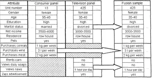
Data fusion is initiated by two (or more) samples, one usually of ]arger size than the other, with the number of individuals appearing in both samples (i.e., the overlap) clearly negligible. Only certain variables, Jet us denote them by Z, of the interesting individual's characteristics can be observed in both samples; they are called common variables. Some variables, Y, appear only in one sample, while other variables, X, are observed exclusively in the second sample; X and Y are called specific variables. F or the purpose of generalization X, Y and Z can be regarded as vectors of variables. In media practice, social dass, housing conditions, marital status, terminal age of education, education, and many other variables as well as gender and age would be used as Z variables for a linking mechanism. Figure 1 illustrates the principle of statistical matching on a simplified example.

Since no single sample exists with information on X, Yand Z together, an artificial sample has tobe generated by matching the observations ofboth samples according to Z. The objective of data fusion is the creation of a complete microdata file where every unit provides observations of all X, Y and Z variables. Once the data are matched the analysis proceeds as ifthe artificial fusion sample is a real sample representative for the true population of interest. Often the data are designed tobe used by many analysts for many different purposes or, finally, become a public resource.

In the last decades, papers have been published showing that traditional data fusion techniques establish the so-called conditional independence, see especially RüDGERS (1984) or for a more detailed discussion RÄSSLER (2002). Under conditional independence the variables never jointly observed are independent given the variables observed in both files after the fusion is performed. Referring to Figure 1 in the artificial fusion sample we find the TV viewing and the purchasing behavior being more or less (conditionally) independent given the demographic and socioeconomic information. So the gain of statistical matching is known a priori.

What is the controversy about? From an information-theoretic point of view it is

Attribute consumer panel

Unit number 13

Gender female

Age 35-40

Education high

Marita! status rnarried Net income 3500-4000

Res1aence row r,ouse

Pets yes

Purchases cereals 1 kg per week Purcr,ases w1ne 3 1 per week Purchases rneat 2 kg perweek

Rents cars

lal

Views daily soaps V1ews news Zaps advertisernent

Fig. 1. Illustration of statistical matching.

© VYS. 2003

Television panel Fusion sample

425 425 ...

female female

35-40 35-40

high high

d1vorced "'"> ^divorced

3000-3500 3000-3500

row house row house

yes yes

r;:;J~/,-;'0//,/~ 1 kg per week

=->--

^{3 1 perwee,,}

r</%;,;,0~/0 ¼/'.I 2 kg perweek

no no

no

-

^no

1 hour per day

-

1 hour per day

yes yes

easy to accept that the association of variables never jointly observed cannot be estimated from the observed data. RUBIN (1974) shows that whenever two variables are never jointly observed, the parameters of conditional association between them given the other variables are inestimable by means of likelihood inference.

Nevertheless, many fusion techniques mainly based on nearest neighbor matches have been applied over years. But these traditional approaches to statistical matching establish (conditional) independence. Hence critical voices argue that any data fusion appears to be unnecessary because the outcome is already known.

Moreover, conditional independence is produced for the variables not jointly observed although they may be conditionally dependent in reality. The critics are right so far. On the contrary advocates of data fusion argue, if the common variables are (carefully) chosen in a way that establishes more or less conditional independence among the variables not jointly observed given these common variables, then inference about the actually unobserved association is valid. In terms of regression analysis this implies that the explanatory power of the common variables is high concerning the specific variables.

To derive alternative procedures for matching we treat the data fusion task as a problem of nonresponse. More precisely, the missing information is regarded as missing at random because the missingness is induced by the study design of the separate samples. The missing data are due to unasked questions and the missingness mechanism is regarded as ignorable which in principle makes the application of conventional multiple imputation techniques obvious. Contrary to the usual missingness patterns, data fusion is characterized by its identification problem.

The association of the variables never jointly observed is unidentifiable and cannot be estimated by means of likelihood inference. However, depending on the explanatory power of the common variables Z there is a smaller or wider range of admissible values of the unconditional association of X and Y. Only a few approaches have been published to assess the effect of alternative assumptions of this inestimable value. KADANE (2001) (originally 1978, now reprinted), MüRIARITY and SCHEUREN (2001), and RUBIN (1986) describe regression based procedures to produce synthetic datasets under various assumptions on this unknown association.

A full Bayesian regression approach is given by RUBIN (1987), p. 188. We follow the latter to propose the use ofmultiple imputation (MI) techniques that are either based on informative prior distributions in the Bayesian context to overcome the conditional independence assumption or efficiently exploiting auxiliary data.

If no prior information about the unconditional association is available, we follow RusIN's advice of investigating the sensitivity of the association between X and Y, rather than assuming one prior value for it. Such a prior specification can take a parametric form, e.g., as the partial correlation between X and Y given Z, with the advantage that it is relatively easy to manipulate. lt also allows one to illustrate the explanatory power of the common variables. Another, but related, possibility is that additional data might be found on X, Y, and Z. Matching methodology should be able to take such auxiliary information into account, whenever it's available.

2 Stochastic regression imputation 2.1 Introduction

Many intuitively appealing approaches to imputation in general are based on hot deck, nearest neighbour or regression techniques; e.g., see RUBIN and SCHENKER (1998) or the recent discussions in GROVES et al. (2002). Instead of imputing predicted or observed values from suitable donor units, sometimes a random residual is added to account for the tendency of single imputation techniques to reduce variability. This so-called stochastic regression imputation, for example, can be used to produce multiple imputations. However, such procedures not derived within the Bayesian framework are often not proper in the sense defined by RUBIN (1987), because additional uncertainty due to random draws from the model parameters is missing. Proper MI methods reflect the sampling variability correctly; i.e., the resulting multiple imputation inference is valid also from a frequentist's view.

Roughly speaking, if we get randomization-valid inference with the complete data then a MI method is proper if we get randomization-valid inference with the (theoretically infinitely) multiply imputed data.

In the context of statistical matching, RUBIN (1986) proposed an implicit (i.e., not Bayesian based) regression model concatenating the separate samples and using multiple imputations. Assuming different conditional associations of the specific variables given the common variables multiple imputations are created by means of a predictive mean matching process which was named and extended later by LITTLE (1988). We discuss a similar regression imputation procedure first using random residuals to create multiple imputations for a given conditional association. A füll Bayesian MI model is derived easily then in the following section. Notice that other regression based procedures for assessing the effect of alternative assumptions of the inestimable unconditional association of the specific variables has been published by KADANE (2001) and MoRIARITY and SCHEUREN (2001). The latter also use random residuals in the regression but prior to the matching process. Their matching procedure is performed using the Mahalonobis distance and leads to synthetic datasets which are imputed only once.

2.2 Imputation procedure

Let us consider data fusion as a problem of file concatenation; for illustration see Figure 2 which also introduces the notation used herein.

A regression imputation procedure for the fusion case can be constructed as follows. Assume the general linear model for both datasets with

(file A) Y

=

ZAßyz

+

UA. and (file B) X= Zsßxz

+

Us, (1) with ZA 11.4 x k and Zn ns x k matrices of known values each with rank k. Usually we treat Z as the common derivative matrix including the constant (l,1, ... ,1)', thus, we !et z1 describe the constant. Y and X correspond to any multivariate variables as pictured in Figure 2. X denotes ans x q matrix and Y a n.4 x p matrix according to

© vvs. 200.1

Unit Common varz specific varX Specific var Y no.

<

"

i';; ...

ll:.

"

i';; ...

n

I< common variables Z q specific variables X p specific variables Y Fig. 2. Data fusion pictured as file concatenation.

U = (Z,X,Y) FileA:

Umis = ^(X)

Uobs = (Z,Y) FileB:

Umis = (Y) Uobs = (Z,X)

the general multivariate normal model, see Box and TIAO (1992), pp. 423-425.

Notice that although the common variables Z are usually regarded as being fixed, in a slight abuse of notation, we write

a-t

1z instead of

a-t,

and so on, just to correspond to the distinction between the unconditional association p ^XY of X and Y and the conditional association PxY z of X and Y given Z

=

z.

We assume a multivariate normal data model for (X,YIZ

=

z)

=

(X1, X2, .. -,Xq, Y1, Y2, ... , YplZ

=

z) with a given common variable Z

=

z and the parameters are also given. The expectation is µxyz and the covariance matrix Ixy z is denoted by

o-x,xi1z o-x,XqlZ O"x, YtlZ o-x, YplZ

O"XqXt IZ O"x"x"1z O"XqYtlZ o-xqYplZ

=

(I11 I12) Ixr1z

=

o-y,x,1z O"y,XqlZ O"y, YtlZ O"y, YplZ I21 I22 ' (2)

O"ypx, 1z O"ypXqlZ O"ypyl IZ O"ypyplZ

then the residual VA

~

^{Np11)0, I:22 @ 111 ) and VB}

~

^{Nq11/0, I 11 @ /118). Sometimes}

we set I 11

=

Ix z, I:22

=

I y z. This data model assumes that the units can be observed independently for i

=

1, 2, ... ,n. The correlation structure refers to the variables Xli, X2i,···,Xqi, Yli, Y2i, ... , Ypi for each unit i

=

1, 2, ... ,n. For abbreviation we use the Kronecker product ^@ denoting that the variables Xi and Y;

of each unit i, i

=

1, 2, ... ,n, are correlated but no correlation of the variables is assumed between the units.

The maximum likelihood (or ordinary least squares) estimates derived from the data model are

ßyz =

(Z~ZA)-' Z~ Y and l3xz

=

(Z~Zs)-¹ Z~X. With the multi- variate X and Y we get a k x p matrix of parameters {J yz as well as a k x q matrix of parameters ßxz- Using the estimates

ßrz

and

ßxz

the residual matrices I:11 and I:₂₂ can be estimated for each regression with

Sy/(nA - k)

=

(Y - ZAßyz)'(Y - ZAßyz)/(nA - k)

=Ln=

Lr1z

= {

8-r,r11z}, i,j = 1, 2, ... ,P

Sx/(ns - k)

=

(X - Zsßxz)'(X - Zsßxz)/(ns - k)

=

:t,

^{1 = Lx1z = { 8-x,xj)Z }, i,j}

⁼

^{1, 2, ... , q. (3)}

Now we refer to the linear regression of Xon Z and Y for file A and Y on Z and X for file B, respectively. Thus we model

(file A) X= ZAßxz y + Yßxr.z + V,i, V,i

~

Nn,q(O, Ix1zr 0 In,),

(file B) Y

=

Zsßrzx +Xßyx.z

+

Vs, Vs~ Nn8p(O,Ir1zx 0In8 )- (4) To estimate the parameters of (4) we first calculate the conditional covariance matrix fxYIZ· Therefore any 'prior' information may be used to fix the conditional correlation matrix Rxy,z,

· · · Px,~,IZ)

. · · . · · =

{pX,YJIZ},

· · · PxqYplZ (5)

for i

=

1, 2, ... ,q, j

=

1, 2, ... ,p denoting a matrix of size ^q x ^p. Notice that this re- gression imputation method is not based on Bayesian inference. Thus, prior infor- mation refers to any arbitrarily chosen values for the conditional correlation of X and Y given Z

=

z. The estimate of I 12 is calculated by means of (3) with

(6) (7) The regression parameters for (4) are derived according to Cox and ^WERMUTH (1996), p. 69, with

(file A) ßxz.Y = ßxz - ßrzßxY.Z with ßxr.z = f;1hf21, and (file B) ßrzx

=

ßrz - ßxzßYJc.z with ßyx.z =

fx1~L12.

The predicted regression values of all X and Y variables are given by (file A) X= XA

=

ZAßxzy

+

Yßxrz,

Y = YA = ZAß}zx

+

XAßrx.z, (file B) Y

=

Ys

=

Zsßnx

+

Xßrx.z, and

X= Xs

=

Zsßxz.r + Ysßxr.z·

(8)

(9) The residual variances Ix zy and Iy!zx of the regression (4) can be estimated using (9)

© VVS. 2003

'tr1zx

=

(Y - Y)'(Y - Y)/(nA - (k

+

q)) with Y, Y

=

YA taken from file A 'tx1zr

=

(X -X)'(X -X)/(ns - (k

+

p)) with X, X= Xs taken from file B.

Random residuals can be generated according to VAJ

~

^{Nq(O, i: X\ZY) for each}

single row i

=

1,2, ... ,nA and

VB.i ~

^{Np(O, i:y1zx)} for each single row i

=

1,2, ... ,ns.

More generally, we write VA

~

^Nq„A (0, fx1zy @ InA) and Vs

~

^Np„8(0, 'ty1zx

@J„_{8 ).} These randomly generated values are added to the regression output.

Finally, the imputed values are

(file A) X= ZAßxz.r

+

Yßxr.z

+

°V4,

(file B) Y

=

Zsßrzx +Xßrxz

+

^{Vs. ( 10)}

The calculation of the imputed values according to (10) is equivalent to drawing the missing values from their conditional predictive distribution/u,,,;,IU,,1,,,0(u111;, ^J Uahs, 0) given the observed data and some actual parameter values

0,

^i.e.,

(file A) X[y

~

^Nqn, (f1x1m 'tx1zr ® I„A) and (file B) Y[x

~

^Npns (11r1zx, 'tr1zx ® I„s) with

.

.

.

.

·,·

/1x1zr = ZAßxz y

+

Yßxr.z = ZAßxz

+

(Y - ZAßdLr1zL21,

• • • • • l •

h1zx = Zsßrzx +Xßrxz = Zsßrz

+

(X -Zsßxz)Lx1zL12-

( 11)

In this frequentist regression imputation with random residual, called RIEPS hereinafter, the missing values are imputed according to (11). The parameters are estimated from the observed data as described above.

2.3. Discussion

Regression imputation is a computationally interesting approach, because neither random draws for the parameters nor iterations to achieve any stationary distribution are necessary. Despite its computational advantages and its general acceptance among practitioners, this imputation procedure is not proper because the parameters are not randomly drawn according to their observed-data posterior. Roughly speaking, regression imputation often yields to biased estimates due to its lack of asymptotic properties. In the following section we extend this approach to its Bayesian version, performing random draws for the parameters instead of estimating them.

3 Non-iterative multivariate imputation procedure 3.1 Introduction

Extending the regression imputation procedure already proposed we now introduce a new non-iterative Bayesian based imputation procedure which is Bayesianly proper by definition. For short we call it NIBAS hereinafter. The elements of each column

·'f: \'\'S. 2003

of the common matrix Z can either be an appropriate sequence of -1 's, 0's or l 's corresponding to a design matrix, or contain 0's and l 's describing some qualitative variables, or, finally, may simply contain continuous values. Being quite general, we only require Z tobe suitable to serve as predictor matrix in a linear regression model.

Concerning the specific variables X and Y our assumptions are more restrictive. Here we require variables that may be regarded as, at least, univariate normally distributed. Variables concerning media and consuming behavior may fulfill this demand after applying some useful transformations.

3.2 Imputation procedure

Again we assume the general linear model for both datasets with (file A) Y

=

^ZAßiz

+

U.4,

(file B) X= Zsßxz

+

^{Us, UA Us}

^~

^~Nq11Npn, 8^(0, (0,L11 ^{L22 ®} @Ins), ^111,), ( 12) with ZA and Z8 denoting the corresponding parts of the common derivative matrix Z. Again we assume a multivariate normal data model for (X, YIZ

=

z)

=

_{(X1,X2, ..}. ,Xq, Y1, Y2, ... , Yp I Z

=

z) with expectation JlXY'Z and co- variance matrix Lxy z like (2). As a suitable noninformative prior we assume in- dependence between

ß

and

:r

choosing

( 13)

RÄSSLER (2002) shows that the joint posterior distribution for the fusion case can be factored into the prior and likelihood derived by file A and file B, respectively. Then the joint posterior distribution can be written with fßxz-fl,z. I,-z. r,;z,Rxr,zlx.Y

=

^{Ci 1}

L(ßxz, Lx1z; x) fz., ^{z Rn z}

cy

¹ L(ßyz, Lyrz; y)

h,

^z I Rxy z fR,, ^z·

Thus, our problem of specifying the posterior distributions reduces to standard derivation tasks described, for example, by Box and TIAO (1992), p. 439. Lx z and Lyz given the observed data each is following an inverted-Wishart distribution. The conditional posterior distribution of ß xz (ß yz) given Lx z (L y z) and the observed data is a multivariate normal distribution. The posterior distribution of Rxv,z equals its prior distribution. Having thus obtained the observed-data posteriors and the conditional predictive distributions a multiple imputation procedure for multivariate variables X and Y can be proposed with algorithm NIBAS.

Algorithm 'NIBAS'

• Compute the ordinary least squares estimates

ßrz

= (Z~ZA)-1_{Z~Y, and}

ßxz

= (Z~Zs)-1_Z~X

from the regression of each dataset. Note that

ßiz

is a k x p matrix and

ßxz

is a k x q matrix of the OLS or ML estimates of the general linear model.

© VVS. 2003

• Calculate the following matrices proportional to the sample covariances for each regression with

Sy

=

(Y - ZAßyz)'(Y - ZAßyz), and Sx

=

(X - Zsßxz)'(X - Zsßxz).

• Choose a value for the correlation matrix Rxy '. z or each Px,v_{1 1,} z for i = 1, 2, ... ,q, j = I, 2, ... ,p either

(a) from its prior according to some distributional assumptions, e.g., uniform over the p + q-dimensionalJ-1, l [-space, or

(b) several arbitrary levels, or

(c) estimate a value from a small but completely observed dataset.

• Perform random draws for the parameters from their observed-data posterior distribution according to the following scheme:

Step 1:

I:22\Y

~ w;

^{1 (vA,Sr1) with vA}

⁼

^{nA - (k}

⁺

^p)

⁺

^1,

I1ilx"' W;1(vs,Sx1) with Vs= ns - (k+ q) + l.

Step 2:

ßn\I22,Y

~

Npk(ßrz, Ln 0 (Z,~ZA)-1), ßxzlill,x

~

^{Nqk(ßxz, L11 0} (Z~Zs)-1).

Step 3:

Set L12

=

{o-x11;1z} with o-x;Y1Jz

=

Px1r;1z o}₁zo-bz with o-ii1z, o-t₁z derived by step 1 fori= 1,2, ... ,q, J= 1,2, ... ,p.

Step 4:

X!y,ß,I.

~

^Nq11,(ZAßxz

+

(Y- ZAßyz)L

2

^iL21;

(L11 - L12I

22

^{1I21) ®111}

J

Ylx, ß, I

~

^Np118(Zsßrz

+

(X -Zsßxz)L

1

^}L12;

(I22 - I.21I

1

^{([12) ?91118 ).}

Repeating this procedure 111 times yields 111 imputed datasets which can be analyzed by standard complete data inference. The results are combined then according to the MI paradigm. As proposed by RUBIN to create suitable imputations (e.g., see RUBIN,

1987 or RUBIN and SCHENKER, 1998), we obtain draws for the missing data from their posterior predictive distribution by first drawing values for the parameters from their observed-data posterior distribution and then drawing values for the missing

data from their predictive distribution conditional on the drawn parameter values.

Thus, ourimputations are repetitions from a Bayesian posterior predictive distribution for the missing data. Under the posited response mechanism and when the model for the data is appropriatc, then in !arge samples such an imputation method should be proper for a wide range of standard statistics; for details see RUBIN ( 1987).

The similarity of this new multiple imputation procedure with the stochastic regression imputation method according to ( 11) is obvious. Instead of estimating the model parameters they are drawn from their observed-data posterior distribution.

More uncertainty to account for the missing data is incorporated than by simply adding a random residual. We are also able to influence the resulting imputations by the prior choice of Rxy z. The range of admissible values of Rxy can finally be estimated from the imputed datasets. Thus, it is possible to display the predictive power ofthe common variables Z by this procedure. Notice that in the multivariate case choosing the correlation matrix Rxy z uniform over the p

+

q-dimensional ]-1,1[-space may lead to invalid conditional variances in step 4. To achieve imputations reflecting the bounds of the possible range of the unconditional association between X and Y we propose to set Rxy z

=

0qxp and add some ± ^E iteratively until the variance matrices in step 4 are no longer positive definite. A similar procedure to get admissible values of the covariance matrix is proposed by MORIARITY and SCHEUREN (2001) for the multivariate case. For univariate X and Y variables p xy z may be chosen from J-1, I [. The bounds can be calculated directly then, see also MoRIARITY and SCHEUREN (2001).

3.3 Discussion

We have shown that it is possible for the fusion problem to formulate a suitable data model and prior distribution and to derive the observed-data posterior therefrom. This is due to the special missingness pattern induced by the fusion. We find this approach rather encouraging because it allows a quick and controlled data fusion generating suitable multiple imputations. Further criteria and advantages ofNIBAS are discussed in the following simulation study as weil as in more detail by RÄSSLER (2002).

4 Simulation study

The simulation study described below has three objectives. The first objective is to explore the efficiency of estimating the unconditional association of the variables never jointly observed based on the imputed dataset when different prior information about their conditional association is used. The second objective is to investigate to what extent a third data source of a complete nature may improve the estimation of the unconditional association. Finally, we want to demonstrate the simplicity of application of the proposed fusion techniques and highlight their benefits. For an application of the following Bayesian procedures to real world media data see RÄSSLER (2002).

:0 \'\'S. 2003

4.1 Data model

Let (Z_1, Z_2, X, Y) each be univariate standard normally distributed variables with their joint distribution (Zi, Z2, X, Y)

~

^{Ni0, 1:) and Jet}

1.0 0.2 0.5 l:= 0.2 1.0 0.5 0.5 0.5 1.0 0.8 0.6 O")X

0.8 0.6

(Tyy

1.0 ) (

Lzz Lzx Lzy)

=

l:xz O"xx O"xr , Lrz O"JX O"yy

l:xr=(O";o: O"xr). O"yx O"yy (14)

Throughout the study we assume that the true covariance is given with O"XY

=

^O"yx

=

^0.8. Furthermore, Jet file A = (Z1, Z2, Y) and file B = (Z1, Z2, X), thus X and Y are never jointly observed. As it is shown in ^RÄSSLER (2002) the simple nearest neighbor match leads to conditional independence of X, Y I Z

=

^z with the unconditional covariance after the fusion irxr

=

LxzLziLzy

=

0.5833.

To calculate the unconditional covariance, when a particular conditional correlation is given, the following well-known formula is used:

Lxr

=

Lxr1z

+

^[~xz] _{.... yz} Lzi [LzxLzy] with LXYIZ

= (

O"xxtz O"XYIZ). O"rx1z O"mz ( 15) According to the Cauchy-Schwarz inequality the conditional covariance is bounded by lcrXY1zl

=

J0.5833 · 0.1583

=

0.3039. We calculate some associations according to (15) with Gxy

=

Pxr.z · 0.3039

+

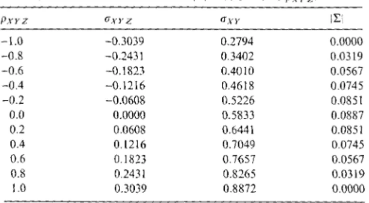
^0.5833 and the corresponding determinant values 11:1 as listed in Table 1. Due to O"xx

=

O"yy

=

1 our setting is p xr

=

a-xr-Hence, only a range of the unconditional correlation of the two variables never jointly observed with Pxr E [0.2794, 0.8872] yields a positive definite matrix l:. Notice that the "conditional independence value" of Pxr

=

0.5833 is the midpoint of the range of admissible values of Pxr and maximizes Wilks' generalized variance; i.e., the determinant 11:1 of the covariance matrix as given above with all other parameters fixed.

Table l: Values of the determinant [LI as function of PxY z.

PxYZ uxyz UX}' iLi

-1.0 -0.3039 0.2794 0.0000

-0.8 -0.2431 0.3402 0.0319

-0.6 -0.1823 0.40 lO 0.0567

-0.4 -0.1216 0.4618 0.0745

-0.2 -0.0608 0.5226 0.085!

0.0 0.0000 0.5833 0.0887

0.2 0.0608 0.6441 0.0851

0.4 0.!216 0.7049 0.0745

0.6 0.!823 0.7657 0.0567

0.8 0.243! 0.8265 0.03!9

1.0 0.3039 0.8872 0.0000

fJ \'VS. ~003

4.2 Design of the study

We draw n

=

5000 random numbers for (:, x, y) according to (Z, X, Y)

~

N4(0, I:).

This generated dataset is divided into two parts, each file of size 2500 and all x (file A) or ^y (file B) values are eliminated. Then we either assume different conditional correlations of X and Y given Z

= :

as prior information or take another random draw to generate a small but complete data source.

The multiple imputation procedures implemented for this study are as follows.

• NORM, the data augmentation algorithm assuming the normal model as proposed by SCHAFER (1997, 1999) is applied based on m

=

5 multiple imputations. Using the S-PLUS library NORM we run a burn in period of 100 iterations, then impute the missing data from every further 50th iteration.

• NIBAS, the non-iterative multivariate Bayesian regression model based on m

=

5 multiple imputations is used.

• An iterative univariate imputation method proposed by VAN BuUREN and OuDSHüüRN (1999, 2000) implemented as S-PLUS library MICE is applied.

Note that MICE does not allow the use of informative (parametric) priors as it does not rely on a parametric prior distribution for the parameters. This is typical for many of the actually available MI routines. The default settings of the S-PLUS function 'mice()' are taken here.

• RIEPS is the regression imputation technique discussed in section 2. For the fusion task we are able to introduce prior information. Moreover, regression imputation is fairly widespread among practitioners, thus, RIEPS may serve as the baseline here.

All computations are basically performed with S-PLUS 2000, copyrighted by MathSoft, Inc. Within NIBAS the prior conditional correlation

Pi·n;

is used directly in step 3 ofits algorithm. For NORM the unconditional covariance

a1;·r

is calculated according to

d;-~,.

^{= üj·;;·z}

+ fxzf2,kfzy

^with

~~-n;

⁼ P:~-~;Ja-x~1z8-yy1z and the covariances being estimated from all available data; i.e., 8-xxiz and L'.xz from file A, 8-yy1z and fzy from file B and

fzz

using all values of Z from the available datasets. Finally,

O'j·t

is taken as the starting value for the data augmentation algorithm itself to fix this parameter. Within RIEPS, the prior setting of

!Tj·;;·z

^is

used to retain the correct regression coefficient for the regression of Xon Z and Y in file A and Y on Z and Y in file B according to (6).

The whole procedure of generating and discarding data, predicting the missing values as described above m

=

5 times for each generated dataset, calculating the usual multiple imputation estimates

eMI ⁼ +, z:::;'~

^{1 9(t)} of the parameters 0 = Ütx, /ly, crxx, cryy, PxY) for each imputed dataset, is repeated k = 50 times.

Note that NORM and NIBAS are computationally rather speedy algorithms, but MICE is not; thus we decided to restrict the repetitions to k

=

50. The within- imputation variance W

=

1-

I::7~

1 var(e(r)) and the between-imputation variance

' ( ) A III

B = 111 ~ 1

I::7~

1(8^{1 -} 8MI)2 are computed k = 50 times. The 95% MI interval

estimates are calculated with

0.,n ± flt

0_975.l', T

=

W + (1

+ m-

¹)B, and degrees

© VYS. 2003

of freedom v

=

(m - 1) ( 1

+

^(l

+!~

^{1 )B}

)2.

This enables us to countthe coverage; i.e., the number of times out of k that cover the true population parameter 8. To ease the reading we display the percentage. According to the MI principle we must assume that based on the complete data the point estimates

0

are approximately normal with mean 8 and variance var(0). Therefore some estimates should be transformed to a scale for which the normal approximation works well. For example, the sampling distribution of the, correlation coefficient PxY

=

&XY/ J&xx&n is known to be skewed, especially if the corresponding correlation coefficient of the population is large. Thus, usually the multiple imputation point and interval estimates of a correlation p are calculated by means of the Fisher .:-transformation z(p)

=

0.5 ln (\

~i),

which makes z(p) approximately normally distributed with mean z(p) and constant variance 1 /(n - 3), see, e.g., SCHAFER (1997), p. 216, or BRAND (1999), p. 116. By back transforming the corresponding MI point and interval estimates of z via the inverse Fisher transformation the final estimates and confidence intervals for p are achieved.

4.3 Results based an prior iriformation

The results are presented in detail in RÄSSLER (2002). Here we focus on the MI estimate PMI

=

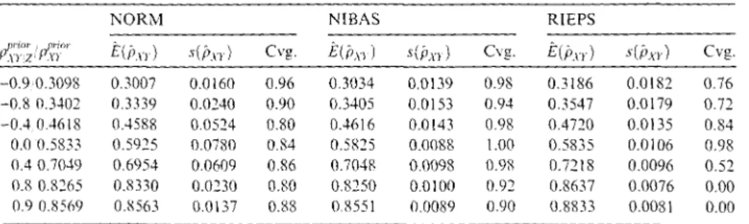
PXY of the unknown association of X and Y. The estimated expectation E(pXY), the standard error s(pXY), denoted by

- - - 1 ~(,()) ^{A A} 2

s(pXY)

= =

k _ l L.., PXY - E(pXY)) ,

J=l

and the coverage from our k

=

50 repetitions of the (back transformed) uncondi- tional correlation for each procedure are listed in Table 2.

When calculating a t-statistic according to t

=

v1c(E(pXY) - r!;t)/s(pXY) to ease interpretation, we realize that with NORM and NIBAS only

P'.;1

_1·2

=

^-0.9 of the settings above yields an absolute value of t greater than three, whereas RIEPS only once under conditional independence has a t-value of less than three. The prior specified value of PxY z, and, thus, also the value of PxY, is well maintained by these procedures. Therefore, the entire range of admissible values of the unknown

Table 1: Simulation study using prior information.

NORM NIBAS RIEPS

l~'.;,o; / ,~:rr

E(i>1rl ^{s(j,n) Cvg.} E(i>xil s(i>xr) ^Cvg. E(i>xrl s(i>xrl ^Cvg.

-0.9 0.3098 0.3007 0.0!60 0.96 0.3034 0.0139 0.98 0.3!86 0.0!82 0.76 -0.8 0.3402 0.3339 0.0240 0.90 0.3405 0.0153 0.94 0.354 7 0.0179 0.71 -0.4 0.4618 0.4588 0.0524 0.80 0.4616 0.0!43 0.98 0.4720 0.0135 0.84 0.0 0.5833 0.5925 0.0780 0.84 0.5825 0.0088 l.00 0.5835 0.0106 0.98 0.4 0.7049 0.6954 0.0609 0.86 0.7048 0.0098 0.98 0.7218 0.0096 0.52 0.8 0.8265 0.8330 0.0230 0.80 0.8250 0.0100 0.92 0.8637 0.0076 0.00 0.9 0.8569 0.8563 0.0137 0.88 0.8551 0.0089 0.90 0.8833 0.0081 0.00

,. \'\"S. :no~

association is reproduced quite weil by the non-iterative multivariate Bayesian regression and the data augmentation procedures. The reproduction is a little bit better and the between-imputation variance is a bit smaller with NIBAS. In the absence of any prior information MICE will assume conditional independence of X and Y given Z. See Table 3.

lt seems to be a challenging area for further research to make the MICE library flexible to informative prior distributions.

4.4. Results based on an auxiliary data file

Now we make use of a third data source. While setting the true PxY

=

0.8 again we draw a small but complete dataset for (z, x, y) according to (Z, X, Y)

~

^{N4C0, L).}

For imputations via NORM and MICE the complete data are simply added to the incomplete data and their imputation procedures are performed based ⁰¹¹ the usual improper priors. For MICE the number of iterations is set to 250 (150) for the n

=

50 (250) auxiliary file leading to a runtime of about 3 hours for each simulation run on an AMD Duron 750 MHz computer. With NIBAS and RIEPS the conditional correlation p ^XYIZ is estimated by means of the small sample first. We estimate CTxy from this third data source and calculate irxy1z according to il'n1z

=

^{il'xy -} fxz:tzi:tzy. Then PXYIZ is derived by PXYIZ

=

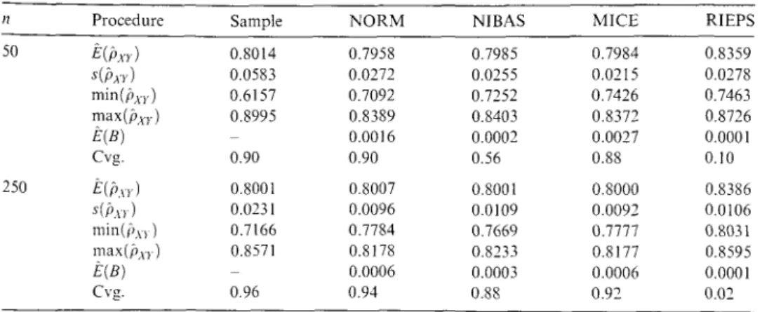
&XY1z/ J&xx1z&n1z and used as prior in step 3 of algorithm NIBAS or to calculate the regression coefficient for RIEPS according to (6).

Table 4 displays the mean estimate of the unconditional correlation and further statistics when samples of 1 % and 5% of the actual sample are available to improve

Table 3: MICE: Simulation study assuming conditional independence.

t11;1;

^{{¼;.or E(PXY) S(f!XY) Cvg.}

0.0 0.5833 0.5751 0.0146 0.96

Table 4: Simulation study using a third data source.

11 Procedure Sample NORM NIBAS MICE RIEPS

50 E(Pxrl 0.8014 0.7958 0.7985 0.7984 0.8359

s(fl.nl 0.0583 0.0272 0.0255 0.0215 0.0278

min(Pxrl 0.6157 0.7092 0.7252 0.7426 0.7463

max(f!xr) 0.8995 0.8389 0.8403 0.8372 0.8726

E(B) ^0.0016 0.0002 0.0027 0.0001

Cvg. 0.90 0.90 0.56 0.88 0.10

250 E(p\T) ^{0.8001 0.8007 0.8001 0.8000 0.8386}

s(f11rl 0.0231 0.0096 0.0109 0.0092 0.0106

min(i,xrl 0.7166 0.7784 0.7669 0.7777 0.8031

max(fl.nl 0.8571 0.8178 0.8233 0.8177 0.8595

E(B) ^0.0006 0.0003 0.0006 0.0001

Cvg. 0.96 0.94 0.88 0.92 0.02

'.0 VYS. 2003

the imputation procedure. We see from Table 4 that even a very small sample of size n

=

50 is suitable to substitute the arbitrary prior used before and, thus, improves the imputation procedure. lt is worth taking all the information provided by the two files into account then basing the estimation on the small third file alone. The range of the correlation estimate derived from the small 1 % sample is considerably narrowed from

p;;iple

^E [0.6157, 0.8995] to the smaller intervals of

P~?RM

^E [0.7092, 0.8389],

i>1ifAS

^E [0.7252, 0.8403] and

Mf?CE

E [0.7426, 0.8372]

by using the proposed procedures. RIEPS usually overestimates the true correlation with a negligible between-imputation variance. Now the coverage is best with NORM. NIBAS produces rather small MI interval estimates due to its rather small between-imputation variance and therefore does not yield the best coverage. This might be due to the fact that estimating the prior value from auxiliary data is an ad hoc specification rather than a correct empirical Bayes procedure; this is left to future research.

4.5 Summary

Since all estimates used here are at least asymptotically unbiased and the sample size is quite !arge, the coverage of the MI interval estimate gives a good hint as to whether the implemented procedure may be proper. If the multiple imputations are proper the actual interval coverage should be equal to the nominal interval coverage.

Concerning the marginal distributions NORM, NIBAS and MICE are apparently proper but only NORM (the S-PLUS library) and NIBAS are capable of including prior information in a parametric form; for details also concerning the preservation of other properties see RÄSSLER (2002). RIEPS provides the lowest coverage due to the fact that variances are often under- and correlations are over-estimated. Whether the parameters of the model are sampled from their complete or observed-data posterior distribution, the extra amount of uncertainty induced thereby improves the validity of the imputation techniques considerably. A third data source is best exploited by NORM and MICE here because the between-imputation variance based on NIBAS is small throughout. By means of the simulation study we have realized that RIEPS is not a proper imputation method even if the data follow simplifying assumptions; i.e., for example, if the data are generated according to the data model assumed. MICE has its disadvantages concerning speed and utilizing (parametric) prior information. If the normal model fits to the data or prior assumptions about the association of the variables never jointly observed others than conditional independence are suitable, we propose to use NORM or NIBAS for the imputation process, otherwise MICE is a rather flexible alternative at hand.

5 Concluding remarks

In the fusion task which can be viewed as a very special missing data pattern, the observed-data posterior distributions is derived under the assumption of a normal

z ,·Ys. 200:,

data model. Thus, a particular model specially suited for the fusion task is postulated. The assumption of normality seems to be a great limitation at first glance but an application to real media data shows rather encouraging results, see RÄSSLER (2002). The iterative univariate imputation procedure MICE tries to reduce the problem of dimensionality to multivariate regressions with univariate responses. lt is a very flexible procedure allowing different scales for the variable of interest.

(Parametric) prior information cannot be used efficiently here. Another great advantage of the alternative approaches proposed herein we find in the property of multiple imputations to reflect the uncertainty due to the missing data. By means of MI it is possible to estimate the bounds of the unconditional association of the variables never jointly observed by using different prior settings. Furthermore, we have seen that prior information is most easily used by NIBAS whereas RIEPS does not impute enough variability. MICE does not allow the use of (parametric) prior information yet. With NORM prior information can only be applied via the hyperparameter when the standalone MS-Windows™ version is used. In the simulation study auxiliary data are most efficiently used by NORM and MICE and third by NIBAS.

References

Box, G.E.P. and G.C. TIAO (1992), Bayesian inference in statistical analysis, John Wiley and Sons, New York.

BRAND, J.P.L. (1999), Development, implementation and evaluation of multiple imputation strategies for the statistical analysis of incomplete data sets, Thesis Erasmus University Rotterdam. Print Partners Ispkamp, Enschede.

Cox, D.R. and N. WERMUTH (1996), Multirariate depe11de11cies, Chapman and Hall, London.

GROVES, R.M., D.A. DILLMAN, J.L. ELTINGE and R.J.A. LITTLE (2002), Survey nonresponse, Wiley, New York.

KADANE, J.B. (2001), Some statistical problems in merging data files, Journal of Ofjicia!

Statistics 17, 423--433.

LITTLE, R.J.A. (1988), Missing-data adjustments in !arge surveys, Jo11rnal of Business and Economic Statistics 6, 287-296.

MoRIARITY, C. and F. ScHEUREN (2001 ), Statistical matching: a paradigm for assessing the uncertainty in the procedure, Jo11rnal of Official Statistics 17, 407--422.

RÄSSLER, S. (2002), Statistical matching: a _fi-equentist theory, practical applications, and al- ternative Bayesian approaches. Lecture Notes in Statistics 168, Springer, New York.

RODGERS, W.L. (1984), An evaluation of statistical matching, Journal of Business and Econometric Statistics 2, 91-102.

RUBIN, D.B. (1974), Characterizing the estimation ofparameters in incomplete-data problems, Journal of the American Statistical Association 69, 467--474.

RUBIN, D. B. (1986), Statistical matching using file concatenation with adjusted weights and multiple imputations, Jo11rnal of Business and Economic Statistics 4, 87-95.

RUBIN, D.B. (1987), Multiple imputationfor nonresponse in sun·eys, John Wiley and Sons, New York.

RUBIN, D.B. and N. SCHENKER (1998), Imputation, in S. KOTZ, C.B. READ, and D.L. BANKS (eds.) Encyclopedia of Statistical Sciences, Update, Volume 2, John Wiley and Sons, New York, 336-342.

1'J VVS. 2003

SCHAFER, J .L. (1997), Analysis of incomplete multivariate data, Chapman and Hall, London.

ScHAFER, J.L. (1999), Multiple imputation under anormal model, Version 2, software for Windows 95/98/NT, available from http:/ /www.stat.psu.edu/jls/misoftwa.html.

VAN BuuREN, S. and K. OuosHOORN (1999), Flexible multivariate imputation by MICE, TNO Report PG/VGZ/99.o54, Leiden.

VAN BuuREN, S. and C.G.M. OuosHO0RN (2000), Multivariate imputation by chained equations, TNO Report PG/VGZ/00.038, Leiden.

Received: February 2002. Revised: August 2002.

f: \'VS. 200.1