Teaching the principles of statistical dynamics Kingshuk Ghosh and Ken A. Dill

Teaching the principles of statistical dynamics

Kingshuk Ghosh and Ken A. Dill

Department of Biophysics, University of California, San Francisco, California 94143 Mandar M. Inamdar and Effrosyni Seitaridou

Division of Engineering and Applied Science, California Institute of Technology, Pasadena, California 91125

Rob Phillips^a兲

Division of Engineering and Applied Science and Kavli Nanoscience Institute, California Institute of Technology, Pasadena, California 91125

共Received 31 May 2005; accepted 1 November 2005兲

We describe a simple framework for teaching the principles that underlie the dynamical laws of transport: Fick’s law of diffusion, Fourier’s law of heat flow, the Newtonian viscosity law, and the mass-action laws of chemical kinetics. In analogy with the way that the maximization of entropy over microstates leads to the Boltzmann distribution and predictions about equilibria, maximizing a quantity that E. T. Jaynes called “caliber” over all the possible microtrajectories leads to these dynamical laws. The principle of maximum caliber also leads to dynamical distribution functions that characterize the relative probabilities of different microtrajectories. A great source of recent interest in statistical dynamics has resulted from a new generation of single-particle and single-molecule experiments that make it possible to observe dynamics one trajectory at a time.

©2006 American Association of Physics Teachers.

关DOI: 10.1119/1.2142789兴

I. INTRODUCTION

We describe an approach for teaching the principles that underlie the dynamical laws of transport of particles共Fick’s law of diffusion兲, energy 共Fourier’s law of heat flow兲, mo- mentum共the Newtonian law for viscosity兲,¹and mass-action laws of chemical kinetics.² Recent experimental advances now allow for studies of forces and flows at the single- molecule and nanoscale level, representative examples of which may be found in Refs. 3–10. For example, single- molecule methods have explored the packing of DNA inside viruses⁷ and the stretching of DNA and RNA molecules.^9,10 Similarly, video microscopy now allows for the analysis of trajectories of individual submicron size colloidal particles,¹¹ and the measurement of single-channel currents has enabled the kinetic studies of DNA translocation through nanopores.^3,6

One of the next frontiers in biology is to understand the

“small numbers” problem: how does a biological cell func- tion given that most of its proteins and nucleotide polymers are present in numbers much smaller than Avogadro’s number?¹² For example, one of the most important mol- ecules, a cell’s DNA, occurs in only a single copy. Also, it is the flow of matter and energy through cells that makes it possible for organisms to maintain a relatively stable form.¹³ Hence, cells must be in this stable state far from equilibrium to function. Thus, many problems of current interest involve small systems that are out of equilibrium.

Our interest here is twofold: to teach students a physical foundation for the phenomenological macroscopic laws, which describe the properties of averaged forces and flows, and to teach them about the dynamical fluctuations away from those average values for systems with small numbers of particles.

In this article we describe a simple way to teach these principles. We start from the “principle of maximum caliber”

first described by E. T. Jaynes.¹⁴It aims to provide the same

type of foundation for the dynamics of systems with many degrees of freedom that the second law of thermodynamics provides for the equilibria of such systems. To illustrate the principle, we use a slight variant of one of the oldest and simplest models in statistical mechanics, the dog-flea or two urn model.^15–17 Courses in dynamics often introduce Fick’s law, Fourier’s law, and the Newtonian-fluid model as phe- nomenological laws, rather than deriving them from some deeper foundation. We describe an unified perspective that we have found useful for teaching these laws from a foun- dation in statistical dynamics. In analogy with the role of microstatesas a basis for the properties of equilibria, we focus on microtrajectories as the basis for predicting dynamics.

One argument that might be leveled against the kind of framework we present here is that in the cases we consider it is not clear that it leads to anything different from what one obtains using conventional nonequilibrium thinking. On the other hand, restating the same physical result in different language often can provide a better starting point for subse- quent reasoning. This point was well articulated by Feynman in his Nobel lecture:¹⁸

“Theories of the known, which are described by different physical ideas may be equivalent in all their predictions and are hence scientifically indis- tinguishable. However, they are not psychologi- cally identical when trying to move from that base into the unknown. For different views suggest dif- ferent kinds of modifications which might be made and hence are not equivalent in the hypotheses one generates from them in one’s attempt to understand what is not yet understood.”

We begin with the main principle embodied in Fick’s law.

Why do particles and molecules in solution flow from re-

123 Am. J. Phys.74共2兲, February 2006 http://aapt.org/ajp © 2006 American Association of Physics Teachers 123

gions of high concentration toward regions of low concen- tration? To keep it simple, we consider one-dimensional dif- fusion along a coordinate x. The diffusion is described by Fick’s first law of particle transport,^1,2 which says that the average flux 具J典 is given in terms of the gradient of the average concentration⳵具c典/⳵^xby

具J典= −D⳵具c典

⳵^{x , 共1兲}

where D is the diffusion coefficient. To clearly distinguish quantities that are dynamical averages from those that are not, we indicate the averaged quantities explicitly by angular brackets,具…典. Before we describe the nature of this averag- ing and the nature of the dynamical distribution functions over which the averages are taken, we briefly review the standard derivation of the diffusion equation. We combine Fick’s first law with particle conservation,

⳵具c典

⳵^{t = −}

⳵具J典

⳵^{x , 共2兲}

and obtain Fick’s second law, which is also known as the diffusion equation:

⳵具c典

⳵^{t =D}

⳵²具c典

⳵^{x2 . 共3兲}

The solution of Eq. 共3兲subject to two boundary conditions and one initial condition gives具c共x,t兲典, the average concen- tration in time and space, and the average flux具J共x,t兲典when no other forces are present. The generalization to situations involving additional applied forces is the Smoluchowski equation.²

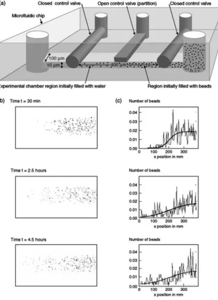
A simple experiment shows the distinction betweenaver- aged quantities andindividual microscopic realizations. By using a microfluidics chip like that shown in Fig. 1共a兲, it is possible to create a small fluid chamber divided into two regions by control valves. The chamber is filled on one side with a solution containing a small concentration of micron- scale colloidal particles. The other region contains just water.

The three control valves on top of that microfluidic chamber serve two purposes: The two outer ones are used for isolation so that no particles can diffuse in and out of the chamber, while the middle control valve provides the partition be- tween the two regions. The evolution of the system is then monitored after the removal of the partition 关see Fig. 1共b兲兴.

The time-dependent particle density is determined by divid- ing the chamber into a number of equal sized boxes in the

Fig. 1. Colloidal free expansion setup to illustrate dif- fusion involving small numbers of particles.共a兲Sche- matic of experimental setup.共b兲Several snapshots from the experiment. 共c兲 Normalized histogram of particle positions during the experiment. The solution to the dif- fusion equation for the microfluidic “free expansion”

experiment is superposed for comparison.

long direction and by computing histograms of the numbers of particles in each slice as a function of time. This system is a colloidal solution analog of the gas diffusion experiments of classical thermodynamics. The corresponding theoretical model usually used is the diffusion equation. Figure 1共c兲 shows the solution to the diffusion equation as a function of time for the geometry of the microfluidics chip. The initial condition is a step function in concentration atx= 200␮m at timet= 0.

We use this simple experiment to illustrate one main point.

The key distinction is that the theoretical curves are very smooth, while there are very large fluctuations in the experi- mentally observed dynamics of the particle densities. The fluctuations are large because the number of colloidal par- ticles is small, tens to hundreds. The experimental data show that the particle concentrationc共x,t兲 is a highly fluctuating quantity. It is not well described by the standard smoothed curves that are calculated from the diffusion equation. Of course, when averaged over many trajectories or when par- ticles are at high concentrations, the experimental data should approach the smoothed curves that are predicted by the classical diffusion equation.

II. THE EQUILIBRIUM PRINCIPLE OF MAXIMUM ENTROPY

Because our strategy follows so closely the Jaynes deriva- tion of the Boltzmann distribution law of equilibrium statis- tical mechanics,^2,19 we first show the equilibrium treatment.

To derive the Boltzmann law, we start with a set of equilib- rium microstates i= 1 , 2 , 3 , . . . ,N that are relevant to the problem at hand. Our aim is to calculate the probabilitiespi

of these microstates in equilibrium. We define the entropyS of the system as

S共兵pi其兲= −kB

兺

i=1 N

pilnpi, 共4兲

wherek_Bis Boltzmann’s constant. The equilibrium probabili- ties,pi=p_i^*are those values ofpithat cause the entropy to be a maximum, subject to two constraints:

兺

i=1 N

pi= 1, 共5兲

which is a normalization condition that ensures that the prob- abilities pisum to one, and

具E典=

兺

_i ^{piEi, 共6兲}

which says that the energies, when averaged over all the microstates, sum to the macroscopically observable average energy.

By using Lagrange multipliers␭and␤to enforce the first and second constraints, respectively, we obtain an expression for the valuesp_i^* that maximize the entropy:^2,19

兺

_i ^{关− 1 − lnpi*−␭−␤Ei兴= 0. 共7兲}

The result is that

p_i^*=e^−␤Ei

Z , 共8兲

whereZis the partition function, defined by

Z=

兺

_i ^{e−␤Ei. 共9兲}

After a few thermodynamic arguments, the Lagrange multi- plier␤can be shown to be equal to 1 /kBT.¹⁹This derivation, first given in this simple form by Jaynes,¹⁹ identifies the probabilities that are both consistent with the observable av- erage energy and that otherwise maximize the entropy.

Jaynes justified this strategy on the grounds that it would be the best prediction that an observer could make, given the observable mean energy, if the observer is ignorant of all else. Although this derivation of the Boltzmann law is now popular, its interpretation as a method of prediction, rather than as a method of physics, is controversial. Nevertheless, for our purposes here, it does not matter whether we regard this approach as a description of physical systems or as a strategy for making predictions.

We switch from the principle of maximum entropy to the principle of maximum caliber.¹⁴In particular, rather than fo- cusing on the probability distribution p共Ei兲 for the various microstates, we seekp关兵␴i共t兲其兴, where␴i共t兲is theith micro- scopic trajectory of the system. Again we maximize an entropy-like quantity obtained from p关兵␴i共t兲其兴to obtain the predicted distribution of microtrajectories. If there are no constraints, this maximization results in the prediction that all the possible microtrajectories are equally likely during the dynamical process. In contrast, certain microtrajectories will be favored if there are dynamical constraints, such as may be specified in terms of the average flux.

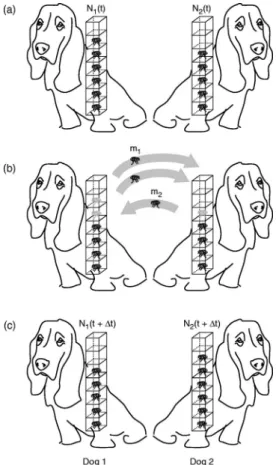
III. FICK’S LAW FROM THE DOG-FLEA MODEL We want to determine the diffusive evolution of particles in a one-dimensional system. The key features of this system are revealed by considering two columns of particles sepa- rated by a plane, as shown in Fig. 2. The left-hand column 1 hasN₁共t兲particles at timetand the right-hand column 2 has N₂共t兲particles. This system is a simple variant of the famous

“dog-flea” model of Ehrenfest’s introduced in 1907.^15,17Col- umn 1 corresponds to dog 1, which hasN₁ fleas on its back at timet, and column 2 corresponds to dog 2, which hasN₂ fleas at time t. In the time interval between time t and t +⌬t, a flea can either stay on its current dog or jump to the other dog. This model has been used extensively to study the Boltzmann H-theorem and to understand how the time asym- metry of diffusion processes arises from the underlying time symmetry in the laws of motion.^15,17,20We use this model for a slightly different purpose. In particular, our aim is to take a well-characterized problem like diffusion and to reveal how the principle of maximum caliber may be used in a concrete way.

First consider the equilibrium state of the dog-flea model.

The total number of ways of partitioning the共N1+N₂兲fleas is W共N1,N₂兲=共N1+N₂兲!

N₁!N₂! . 共10兲

The state of equilibrium is that for which the entropy, S

=kBlnW, is a maximum. A simple calculation shows that the entropy is a maximum when the value N₁=N₁^* is as nearly

equal to N₂=N₂^* as possible. In short, at equilibrium, both dogs will have approximately the same number of fleas, in the absence of any bias.

Our focus here is on how the system reaches equilibrium.

We discretize time into a series of intervals⌬t. We define a dynamical quantityp, which is the probability that a particle 共flea兲jumps from one column共dog兲to the other in any time interval⌬t. Thus, the probability that a flea stays on its dog during the time interval is q= 1 −p. We assume that p is independent of the timetand that all the fleas and jumps are independent of each other.

In equilibrium statistical mechanics, the focus is on the microstates. However, for dynamics we focus onprocesses, which at the microscopic level we call the microtrajectory.

Characterizing the dynamics requires more than just infor- mation about the microstates; we must also consider the pro- cesses. Let m₁ represent the number of particles that jump from column 1 to 2 andm₂represent the number of particles that jump from column 2 to 1 between time t and t+⌬t.

There are many possible values ofm₁andm₂: it is possible that no fleas will jump during the interval⌬t, or that all the fleas will jump, or that the number of fleas jumping will be in between these limits. Each one of these different situations corresponds to a distinct microtrajectory of the system in this idealized dynamical model. We need a principle to tell us what number of fleas will jump during the time interval⌬tat timet. Because the dynamics of this model is so simple, the implementation of the caliber idea is reduced to a simple

exercise in enumeration and counting using the binomial distribution.

A. The dynamical principle of maximum caliber

The probabilityWd共m1,m₂兩N₁,N₂兲 thatm₁ particles jump to the right and that m₂ particles jump to the left in a time interval⌬t, given that there areN₁共t兲andN₂共t兲 fleas on the dogs at timet, is

共11兲 Wd counts microtrajectories in dynamics in the same spirit thatW counts microstates for equilibrium. In the same spirit of the second law of thermodynamics, we maximizeWdover all the possible microtrajectories共that is, overm₁andm₂兲to predict the flux of fleas between the dogs. This maximization is the implementation of the principle of maximum caliber for this model. Maximizing Wd over all the possible pro- cesses 共different values of m₁ andm₂兲 gives our prediction 共right fluxm₁=m₁^*and left fluxm₂=m₂^*兲for the macroscopic flux that we should observe experimentally.共We follow the usual definition of flux, the number of particles transferred per unit time and per unit area. For simplicity, we take the cross-sectional area to be unity.兲

Because the jumps of the fleas from each dog are indepen- dent, we find the predicted macroscopic dynamics by maxi- mizing Wd₁ and Wd₂ separately, or for convenience their logarithms:

冏

^⳵ln⳵^mWi^di

冏

N,m_i=m_i^*

= 0 共i= 1,2兲. 共12兲

The application of Stirling’s approximation to Eq.共11兲gives lnWd_i=milnp+共Ni−mi兲lnq+NilnNi

−m_ilnm_i−共N_i−m_i兲ln共N_i−m_i兲. 共13兲 We callC= lnW_dthe caliber. MaximizingCwith respect to m gives

⳵^lnWd_i

⳵^mi

= lnp− lnq− lnm_i^*+ ln共N_i−m_i^*兲= 0. 共14兲 This result may be simplified to yield

ln

冉

^Ni^m−^i*m_i^*

冊

^{= ln}

冉

^{1 −pp}

冊

^{, 共15兲}

which implies that the most probable jump number is simply given by

m_i^*=pNi. 共16兲

Because our probability distributionW_d is nearly symmetric about the most probable value of flux, the average number and the most probable number are approximately the same.

Hence, the average net flux to the right is

Fig. 2. Schematic of the simple dog-flea model.共a兲State of the system at timet;共b兲a particular microtrajectory in which two fleas jump from the dog on the left and one flea jumps from the dog on the right;共c兲occupancies of the dogs at timet+⌬t.

具J共t兲典=m₁^*−m₂^*

⌬t =p

冋

^{N1共t兲⌬−tN2共t兲}

册

^{⬇−p⌬x⌬t2⌬c⌬x共x,t兲, 共17兲}

which is Fick’s law for this simple model with the diffusion coefficient given by D=p⌬x²/⌬t. We have rewritten N₁

−N₂= −⌬c⌬x.

This approach gives us a simple explanation for why there is a net flux of particles diffusing across a plane down a concentration gradient: more microscopic trajectories lead downhill than uphill. It shows that the diffusion coefficientD is a measure of the jump ratep. This model does not assume that the system is near-equilibrium, for example, it does not utilize the Boltzmann distribution law, and thus it indicates that Fick’s law should also apply far from equilibrium. We might have imagined that for very steep gradients, Fick’s law might have been only an approximation and that diffusion is more accurately represented as a series expansion of higher derivatives of the gradient. But at least for the present model, Fick’s law is a general result that emerges from counting microtrajectories. On the other hand, we would expect Fick’s law to break down when the particle density becomes so high that the particles start interacting with each other, thus spoiling the assumption of independent particle jumps.

B. Fluctuations in diffusion

We have shown that the most probable number of fleas that jump from dog 1 to dog 2 between timet andt+⌬t is m₁^*=pN₁共t兲. The model also tells us that sometimes we will have fewer fleas jumping during this time interval and some- times we will have more fleas. These variations are a reflec- tion of the fluctuations resulting from the system following different microscopic pathways.

We focus now on predicting the fluctuations. To illustrate, we first construct a table of Wd, the different numbers of possible microtrajectories, for all the values ofm₁andm₂. To keep the illustration simple, we consider the special case N₁共t兲= 4 and N₂共t兲= 2. We also assume p=q= 1 / 2. Table I lists the multiplicities of all the possible routes of flea flow. A given entry tells us how many microtrajectories correspond to the value ofm₁andm₂.

Table I confirms our previous discussion. The dynamical process for whichWdis a maximum共12 microtrajectories in this case兲 occurs when m₁^*=pN₁= 1 / 2⫻4 = 2, and m₂^*=pN₂

= 1 / 2⫻2 = 1. You can calculate the probability of this flux by dividing Wd= 12 by the sum of entries in Table I, which is 2⁶= 64, the total number of microtrajectories. The result, which is the fraction of all the possible microtrajectories that havem₁^*= 2 andm₂^*= 1, is 0.18. We have chosen an example in which the particle numbers are very small, so the fluctua-

tions are large; they account for more than 80% of the flow.

In systems with large numbers of particles, the relative fluc- tuations are much smaller.

Now look at the top right entry of Table I. This entry says that there is a probability of 1 / 64 that both fleas on dog 2 will jump to the left while no fleas will jump to the right, implying that the net flux for this microtrajectory is back- ward relative to the concentration gradient. We call these

“bad actor” microtrajectories. In these cases, particles flow to increase the concentration gradient, not decrease it.²¹At time t, there are four fleas on the left dog, and two on the right. At the next instant,t+⌬t, all six fleas are on the left dog, and no fleas are on the right-hand dog.

Similarly, if you look at the bottom left entry of Table I, you see a case of superflux: a net flux of four particles to the right, whereas Fick’s law predicts a net flow of only two particles to the right. Table I illustrates that Fick’s law is only a description of the average or most probable flow and that Fick’s law is not always exactly correct at the microscopic level. However, such violations of Fick’s law are of low probability, a point that we will make more quantitative in the following. Such fluctuations have been experimentally measured in small systems.²³

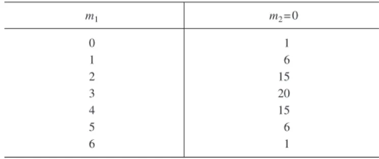
We can elaborate on the nature of the fluctuations by de- fining the “potencies” of the microtrajectories. We define the potency to be the fraction of all the trajectories that lead to a substantial change in the macrostate. The potencies of trajec- tories depend on how far the system is from equilibrium. To see this, we continue our consideration of the simple system of six particles. The total number of microscopic trajectories available to this system at each instant in our discrete time picture is 2⁶= 64. Suppose that at t= 0 all six of these par- ticles are on dog 1. The total number of microscopic trajec- tories available to the system can be classified usingm₁and m₂, where in this case m₂= 0 because there are no fleas on dog 2共see Table II兲.

What fraction of all microtrajectories changes the occu- pancies of both dogs by more than some threshold value, say

⌬Ni⬎1? In this case, we find that 57 of the 64 microtrajec- tories cause a change greater than this value to the current state. We call thesepotenttrajectories.

Now let us look at the potencies of the same system of six particles in a different situation,N₁=N₂= 3 when the system is in macroscopic equilibrium 共see Table III兲. In this case only the trajectories with共m1,m₂兲pairs given by共0,2兲,共0,3兲, 共1,3兲, 共2,0兲, 共3,0兲, and 共3,1兲 satisfy our criterion. Summing over all of these outcomes shows that just 14 of the 64 tra- jectories are potent in this case.

There are two key observations conveyed by these argu- ments. For a system far from equilibrium the vast majority of

Table I. Trajectory multiplicity for the case whereN₁共t兲= 4 andN₂共t兲= 2.

Each entry corresponds to the total number of trajectories for the particular values ofm₁andm₂.

m₁ m₂= 0 m₂= 1 m₂= 2

0 1 2 1

1 4 8 4

2 6 12 6

3 4 8 4

4 1 2 1

Table II. Trajectory multiplicity forN₁共t兲= 6 andN₂共t兲= 0 when the system is far from macroscopic equilibrium. In this casem₂= 0.

m₁ m₂= 0

0 1

1 6

2 15

3 20

4 15

5 6

6 1

trajectories at that time are potent and move the system sig- nificantly away from its current macrostate. Also when the system is near equilibrium, the vast majority of microtrajec- tories leave the macrostate unchanged. We now generalize from the tables to see when fluctuations will be important.

Fluctuations and potencies. A simple way to characterize the magnitude of the fluctuations is to look at the width of the Wd distribution.² It is shown in standard texts that for a binomial distribution for which the mean and most probable value both equalm_i^*=Npi, the variance is␴i2=Nipq. The vari- ance characterizes the width. Moreover, ifNiis sufficiently large, a binomial distribution can be well-approximated by a Gaussian distribution

P共mi,Ni兲= 1

冑

2␲^Nipqexp

冉

^{−共m2Ni−}i^Npq^ip兲2

冊

^{, 共18兲}

a convenient approximation because it leads to simple ana- lytic results. However, this distribution function is not quite the one we want. We are interested in the distribution of flux, P共J兲=P共m₁−m₂兲, not the distribution of right-jumps m₁ or left-jumpsm₂alone.

Due to a remarkable property of the Gaussian distribution, it is simple to compute the quantity we want. If you have two Gaussian distributions, one with mean 具x1典 and variance␴12

and the other with mean具x2典and variance␴2

2, then the dis- tribution function,P共x₁−x₂兲for the difference will also be a Gaussian distribution with mean 具x1典−具x2典 and variance ␴²

=␴₁²⁺␴₂^2.

For our binomial distributions, the means arem₁^*=pN₁and m₂^*=pN₂ and the variances are ␴12=N₁pq and ␴22=N₂pq.

Hence the distribution of the net flux,J=m₁−m₂is P共J兲= 1

冑

2␲共pqN兲exp

冉

^{−共J−p共N2pqN1−N2兲兲2}

冊

^{, 共19兲}

whereN=N₁+N₂.

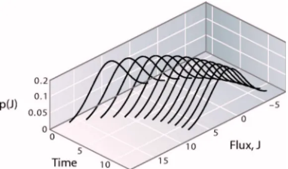
Figure 3 shows an example of the distributions of fluxes at

different times using p= 0.1 and starting from N₁= 100, N₂

= 0. We update each time step using an averaging scheme, N₁共t+⌬t兲=N₁共t兲−N₁共t兲p+N₂共t兲p. Figure 3 shows how the mean flux is large at first and decays toward equilibrium,J

= 0. This result could also have been predicted from the dif- fusion equation. Equally interesting are the wings of the dis- tributions, which show the deviations from the average flux;

these deviations are not predictable from the diffusion equa- tion.

One measure of the importance of the fluctuations is the ratio of the standard deviation␴ to the mean,

冑

_␴²/J. In the limit of large N₁,

冑

_␴²/Jreduces to

冑

^␴J²=

冑

共N1^Npq−N₂兲p⬃N^−1/2. 共20兲 In a typical bulk experiment, the particle numbers are large, of the order of Avogadro’s number 10²³. In such cases, the width of the flux distribution is exceedingly small, and it becomes overwhelmingly probable that the mean flux will be governed by Fick’s law. However, within biological cells and in applications involving small numbers of par- ticles, the variance of the flux can become significant. It has been observed that both rotary and translational single motor proteins sometimes transiently step backward rela- tive to their main direction of motion.²⁴

As a measure of the fluctuations, we now calculate the variance in the flux. It follows from Eq. 共19兲 that 具J²典

=Npq, whereN=N₁+N₂. Thus, we can represent the magni- tude of the fluctuations as

␦⁼

冑

^{具共⌬J兲}具J典^22典=

冑

Npq pfN ⬀1

f

冑

^qpN⁻¹, 共21兲 where N=N₁+N₂ is the total number of fleas and f=共N1

−N₂兲/共N兲 is the normalized concentration difference. The quantity␦is also a measure of the degree of backflux. In the limit of largeN,␦goes to zero. That is, the noise diminishes with system size. However, even whenNis large,␦^{can still} be large 共indicating the possibility of backflux兲 if the con- centration gradient,N₁−N₂, is small.

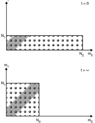
Another measure of fluctuations is the potency. Trajecto- ries that are not potent should have兩m1−m₂兩⬇0, which cor- responds to a negligible change in the current state of the system as a result of a given microtrajectory. In Fig. 4 the impotent microtrajectories are shown as the shaded band for whichm₁⬇m₂. We define impotent trajectories as those for which兩m₁−m₂兩艋h 共hⰆN兲. In the Gaussian model, the frac- tion of impotent trajectories is

⌽impotent⬇

冕

−h h

dJ 1

冑

2␲^Npqexp

冉

^{−共J−共N2Npq1−N2兲p兲2}

冊

^共22兲

=1

2

冉

^erf

冋

^h+共N

^冑

^{2Npq1−N2兲p}

册

^{+ erf}

冋

^h−共N

^冑

^{2Npq1−N2兲p}

册 ^冊

^,

共23兲 and corresponds to summing over the subset of trajectories that have a small flux. To keep it simple, we take p=q

= 1 / 2 for which the probability distribution for the micro- scopic flux m₁−m₂is given by Eq. 共19兲. The choice of his arbitrary and we choose h to be one standard deviation,

冑

N/ 4. Figure 5 shows the potencies for various values of

Table III. Trajectory multiplicity forN₁共t兲= 3 andN₂共t兲= 3 when the system is at macroscopic equilibrium.

m₁ m₂= 0 m₂= 1 m₂= 2 m₂= 3

0 1 3 3 1

1 3 9 9 3

2 3 9 9 3

3 1 3 3 1

Fig. 3. Schematic of the distribution of fluxes for different times as the system approaches equilibrium.

N₁and N₂. When the concentration gradient is large, most trajectories are potent, leading to a statistically significant change of the macrostate, whereas when the concentration gradient is small, most trajectories have little effect on the macrostate.

As another measure of the fluctuations, let us now con- sider the “bad actors”共see Fig. 6兲. If the average flux is in the direction from dog 1 to dog 2, what is the probability we will observe flux in the opposite direction共bad actors兲? We use Eq.共19兲for P共J兲to obtain

⌽bad actors⬇

冕

_−⬁⁰

冑

2␲^1Npqexp

冉

^{−共J−共2NpqN1−N2兲p兲2}

冊

^共24兲

=1

2

冉

^{1 − erf}

冋

^共N

^冑

^{12Npq−N2兲p}

册 ^冊

^{共N2⬎N1兲, 共25兲}

which amounts to summing up the fraction of trajectories for which J艋0. Figure 7 shows the fraction of bad actors for p=q= 1 / 2. Bad actors are rare when the concentration gra- dient is large, and highest when the gradient is small. The discontinuity in the slope of the curve in Fig. 7 at N₁/N

= 1 / 2 is a reflection of the fact that the mean flux abruptly changes sign at that value.

IV. FOURIER’S LAW OF HEAT FLOW

Although particle flow is driven by concentration gradi- ents according to Fick’s law, 具J典= −D⳵^c/⳵x, energy flow is driven by temperature gradients according to Fourier’s law:¹

具Jq典= −␬⳵^T

⳵^{x. 共26兲}

Here,Jq is the energy transferred per unit time and per unit cross-sectional area and ⳵^T/⳵^x is the temperature gradient that drives it. The thermal conductivity¹␬plays the role that the diffusion coefficient plays in Fick’s law.

To explore a simplified version of Fourier’s law that de- pends only on particle transport, we return to the dog-flea model as described in Sec. III. Now columns 1 and 2 can differ not only in their particle numbers,N₁共t兲andN₂共t兲, but also in their temperatures,T₁共t兲andT₂共t兲. For simplicity, we assume that each column is at thermal equilibrium and that

Fig. 4. Schematic of which trajectories are potent and which are impotent.

The shaded region corresponds to the impotent trajectories for whichm₁and m₂are either equal or approximately equal and hence make relatively small change in the macrostate. The unshaded region corresponds to potent trajectories.

Fig. 5. Illustration of the potency of the microtrajectories associated with different distributions ofNparticles on the two dogs. The total number of particlesN₁+N₂=N= 100.

Fig. 6. Illustration of the notion of bad actors. Bad actors are the microtra- jectories that contribute net particle motion that has the opposite sign from the macroflux.

Fig. 7. The fraction of all possible trajectories that go against the direction of the macroflux forN= 100. The fraction of bad actors is highest at N₁

=N/ 2 = 50.

each particle that jumps carries with it the average energy 具mv²/ 2典=kBT/ 2 from the column it left. We again take the cross-sectional area to be unity. In this simple model all en- ergy is transported by hot or cold molecules switching dogs.

The average heat flow at timetis 具Jq典=m₁^*

⌬t共kBT₁/2兲−m₂^*

⌬t共kBT₂/2兲=pkB

⌬t关N1T₁−N₂T₂兴, 共27兲 wherem₁^*andm₂^*are as defined in Sec. III A the numbers of particles jumping from each column at timet. If the particle numbers are identical,N₁=N₂=N/ 2, then

具J_q典= pk_BN

⌬t 共T₁−T₂兲= −␬^⌬_⌬x^T, 共28兲 which is Fourier’s law for the average heat flux for this two- column model. The model predicts that the thermal conduc- tivity is ␬⁼共pkBN⌬x兲/共⌬t兲, which can be expressed in a more canonical form as ␬^=pkBnv_av⌬x in terms of the par- ticle densityn=N/⌬xand the average velocity,v_av=⌬x/⌬t.

Our model gives a value for the thermal conductivity similar to that found in the kinetic theory of gases,¹ ␬

=共1 / 3兲k_Bnv_avᐉ, if ⌬x in our model corresponds to ᐉ, the mean free path.

The factors ofp and 1 / 3 in our model and kinetic theory, respectively, can be reconciled by the following observation.

Kinetic theory deals with the motion of particles in three dimensions so that each particle can move in six possible directions共±x, ±y, ±z兲. As a result, only 1 / 6 of the particles will contribute to the heat flux in our direction of interest.

Also, on the plane of interest there are particles coming in from the positive and negative directions. So the factor of 1 / 6 is increased by two to 1 / 3. In contrast, in our model, the particles move with probability p or stay with probability 1

−p. So the contribution to the flux comes from a fraction p of the particles. The origin of the numerical factors is thus clear.

The numerical factors of 1 / 3 orpare not really important to the point we are trying to make. It is also not fair to read too much into this simple but illustrative model. The key point is that the simple model captures the main physical features of heat flow by appealing to the idea of summing over the weighted microtrajectories available to the system.

V. NEWTONIAN VISCOSITY

Another phenomenological law of gradient-driven trans- port is that of Newtonian viscosity,¹

␶=␩^dvy

dx , 共29兲

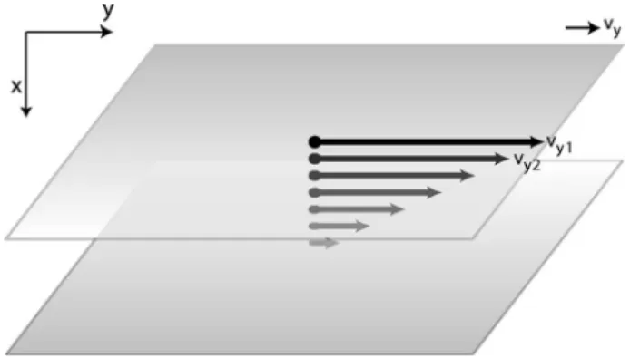
where␶is the shear stress that is applied to a fluid,dv_y/dxis the resultant shear rate, and the proportionality coefficient␩ is the viscosity of a Newtonian fluid. Whereas Fick’s law describes particle transport and Fourier’s law describes en- ergy transport, Eq. 共29兲describes the transport 共in thex di- rection, from the top moving plate toward the bottom fixed plate兲of linear momentum in they direction共parallel to the plates兲 共see Fig. 8兲. In the same spirit as our simplified treat- ment of Fourier’s law, the dog-flea model can be used as the basis of a particle transfer version of momentum transport.

Suppose each particle in column 1 of Table I carries momen- tummvy₁along theyaxis, andm₁^*particles hop from column

1 to 2 at time tcarrying with them some linear momentum.

As before, we consider the simplest model for which every particle carries the same average momentum from the col- umn it leaves to its destination column.

The flux Jp is the amount of y-axis momentum that is transported from one plane to the next in thexdirection per unit area:

具Jp典=m₁^*

⌬t共mvy₁兲−m₂^*

⌬t共mvy₂兲= pm

⌬t关N1vy₁−N₂vy₂兴. 共30兲 If the number of particles is the same in both columns, N/ 2 =N₁=N₂, Eq.共30兲simplifies to

具Jp典=pmN

⌬t 关vy₁−vy₂兴=␩^⌬v_⌬x^y, 共31兲 which is the Newtonian law of viscosity for this two-column model. The viscosity is predicted by this model to be ␩

=共pmN⌬x兲/共⌬t兲. If we convert this result to the more ca- nonical form, we have␩^=pmnvav⌬x, wheren=N/⌬xis the particle density, andv_av=⌬x/⌬tis the average velocity. This form is equivalent to the value given by the kinetic theory of gases,¹␩⁼共1 / 3兲mnᐉvav, if⌬xfrom our model equalsᐉ. The numerical factors of 1 / 3 and pin the kinetic theory and our model, respectively, have the same origin as discussed in the context of heat flow. Note that this simple model based on molecular motions will clearly not be applicable to complex fluids where the underlying molecules possess internal structure.

VI. CHEMICAL KINETICS

WITHIN THE DOG-FLEA MODEL

Let us now look at chemical reactions using the dog-flea model. Chemical kinetics can be modeled using the dog-flea model when the fleas have preference for one dog over the other. Consider the reaction

A

k_r k_f

B. 共32兲

The time-dependent average concentrations, 关A兴共t兲 and 关B兴共t兲are often described by chemical rate equations,²

d关A兴

dt = −kf关A兴+kr关B兴, 共33a兲

Fig. 8. Illustration of Newton’s law of viscosity. The fluid is sheared with a constant stress. The fluid velocity decreases continuously from its maximum value at the top of the fluid to zero at the bottom. There is thus a gradient in the velocity which can be related to the shear stress in the fluid.

d关B兴

dt =kf关A兴−kr关B兴, 共33b兲

wherekfis the average conversion rate of anAto aB, andkr

is the average conversion rate of a B to an A. These rate expressions describe only average rates; they do not give the distribution of rates. SomeA’s will convert toB’s faster than the average ratekf关A兴predicts, and some will convert more slowly. Again we use the dog-flea model and consider the average concentrations and the fluctuations in concentra- tions. A particularly fruitful area for applications of the AB dynamics considered here is to problems involving molecular motors and ion channels.

We assume that dog 1 represents chemical species A and dog 2 represents chemical species B. The net chemical flux from 1 to 2 is given byJc=m₁^*−m₂^*. What is different about our model for these chemical processes than in our previous situations is that now the intrinsic jump rate from column 1 共species A兲,p₁, is different than the jump rate from column 2,p₂. This difference reflects the fact that a forward rate can differ from a backward rate in a chemical reaction. We as- sume that the fleas have a different escape rate from each dog. Fleas escape from dog 1 at ratep₁and fleas escape from dog 2 at rate p₂. Maximizing Wd gives m₁^*=N₁p₁ and m₂^*

=N₂p₂, so the average flux共which is almost the same as the most probable flux because of the approximately symmetric nature of the binomial distribution兲at time tis

具J典=N₁p₁−N₂p₂=kf关A兴−kr关B兴, 共34兲 which is just the standard mass-action rate law, expressed in terms of the mean concentrations. The mean values satisfy detailed balance at equilibrium 共具J典= 0 implies that N₂/N₁

=p₁/p₂=kf/kr兲.

More interesting than the behavior of the mean chemical reaction rate is the behavior of the fluctuations. For example, if the number of particles is small, then even when kf关A兴

−k_r关B兴⬎0, indicating an average conversion ofA’s toB’s, the reverse can happen occasionally. When will these fluc- tuations be large? As in Sec. III, we first determine the prob- ability distribution of the fluxJ. In this case, the probability distribution becomes

P共J兲= 1

冑

2␲共p1q₁N₁+p₂q₂N₂兲

⫻exp

冉

^−共J2共p⁻1^共Nq₁N^1p₁¹+⁻p^N₂²q^p₂N^2兲兲₂兲²

冊

^{. 共35兲}

We use this flux distribution function to consider the fluctua- tions in the chemical reaction. The relative variance in the flux is

具共⌬J兲²典

具J典² =

冑

N₁p₁q₁+N₂p₂q₂

N₁p₁−N₂p₂ . 共36兲 As before, the main message is that when the system is not yet at equilibrium共that is, the denominator is nonzero兲, mac- roscopically large systems will have negligibly small fluctua- tions. The relative magnitude of the fluctuations scales ap- proximately as N^−1/2. Let us also look at the potencies of microtrajectories as another window into the fluctuations. If we use Eq.共23兲withp₁andp₂, we find that the fraction of trajectories that are impotent is

⌽impotent⬇

冕

−h h

dJ 1

冑

2␲共N₁p₁q₁+N₂p₂q₂兲

⫻exp

冉

⁻2共N^共J−1p^共N₁q¹₁^p+¹⁻N^N₂p²₂^pq²₂^兲兲兲²

冊

^共37兲

=1

2

冉

^erf

冋 ^冑

^{2共Nh+共N1p11qp11+−NN22pp22q兲2兲}

册

+ erf

冋 ^冑

^{2共Nh−1共Np11qp11+−NN22pp22q兲2兲}

册 ^冊

^{. 共38兲}

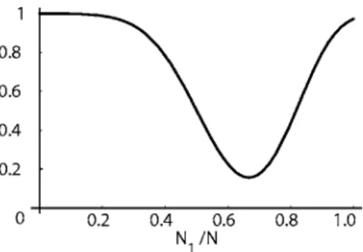
For N₁+N₂=N= 100 and p₁= 0.1 and p₂= 0.2, ⌽potent= 1

−⌽impotentis shown in Fig. 9 as a function of N₁/N.

VII. DERIVATION OF THE DYNAMICAL DISTRIBUTION FUNCTION FROM MAXIMUM CALIBER

We have used the binomial distribution functionW_das the basis for our treatment of stochastic dynamics. The maxi- mum caliber assumption is that if we find the value of W_d that is a maximum with respect to the microscopic trajecto- ries, this value will give the macroscopically observable flux.

We now restate this assumption more generally in terms of the probabilities of the trajectories.

Let P共i兲 be the probability of a microtrajectory i during the interval from timettot+⌬t. A microtrajectory is a spe- cific set of fleas that jump; for example microtrajectory i

= 27 might be the case for which fleas 4, 8, and 23 jump from dog 1 to 2. We take as a constraint the average number of jumps, 具m典, the macroscopic observable. The quantity mi

= 3 in this case indicates that trajectoryiinvolves three fleas jumping. We express the caliberCas

C=

兺

i

P共i兲lnP共i兲−␭

兺

i

miP共i兲−␣

兺

i

P共i兲, 共39兲 where ␭ is the Lagrange multiplier that enforces the con- straint of the average flux and ␣ is the Lagrange multiplier that enforces the normalization condition that theP共i兲’s sum to one. Maximizing the caliber gives the populations of the microtrajectories,

Fig. 9. The fraction of potent trajectories⌽potentas a function ofN₁/Nfor N₁+N₂=N= 100, andp₁= 0.1 and p₂= 0.2. The minimum value of the po- tency does not occur atN₁/N= 0.5, but atN₁/N= 0.66. This value ofN₁/N also corresponds to its equilibrium value given byp₂/共p₁+p₂兲.

P共i兲=e^{−␣−␭mi}. 共40兲 Note that the probability P共i兲 of the ith trajectory depends only on the total number mi of the jumping fleas. Also, all trajectories with the samemihave the same probabilities. In the same way that it is sometimes useful in equilibrium sta- tistical mechanics to switch from microstates to energy lev- els, we now express the populationP共i兲of a given microtra- jectory in terms of ␳共m兲, the fraction of all the microtrajectories that involvemjumps during this time inter- val,

␳共m兲=g共m兲Q共m兲, 共41兲

where g共m兲=N! /关m!共N−m兲!兴 is the density of trajectories with flux m 共in analogy with the density of states for equi- librium systems兲, and Q共m兲 is the probability P共i兲 of mi- crotrajectory i withmi=m. In other words, i denotes a mi- crotrajectory 共a specific set of fleas jumping兲andmdenotes a microprocess 共the number of fleas jumping兲. The total number ofi’s associated with a givenmisg共m兲. It can also be easily seen that

兺

_i ^P共i兲=

兺

m=0 N

g共m兲Q共m兲=

兺

m=0 N

␳共m兲= 1, 共42兲

具m典=

兺

_i ^miP共i兲=

兺

m=0 N

mg共m兲Q共m兲=

兺

m=0 N

m␳共m兲. 共43兲 Thus the distribution of jump-processes written in terms of the jump numbermis

␳共m兲= N!

m!共N−m兲!e^−␣e^−␭m. 共44兲 The Lagrange multiplier ␣ can be eliminated by summing over all trajectories and requiring that⌺m_i=0

N ␳共mi兲= 1, that is,

e^␣=

兺

_m^{N g共m兲e−␭m=}

兺

_m^N _m!共N^N!_−m兲!^{e−␭m=共1 +e−␭兲N. 共45兲}

We combine Eqs.共44兲and共45兲to obtain

␳共m兲= N!

m!共N−m兲! e^−␭

1 +e^−␭. 共46兲

If we now let p= e^−␭

1 +e^−␭, 共47兲

we obtain p^m= e^−␭m

关1 +e^−␭兴^m, 共48兲

and

共1 −p兲^N−m= 1

关1 +e^−␭兴^N−m. 共49兲

If we combine Eqs.共46兲,共48兲, and共49兲, we find the simple form

␳共m兲= N!

m!共N−m兲!p^m共1 −p兲^共N−m兲, 共50兲 which appears in Eq.共11兲and which we have used through- out this paper.

VIII. SUMMARY AND COMMENTS

We have shown how to derive the phenomenological laws of nonequilibrium transport, including Fick’s law of diffu- sion, Fourier’s law of heat conduction, the Newtonian law of viscosity, and the mass-action laws of chemical kinetics from a simple physical foundation that can be taught in under- graduate courses. We used the dog-flea model for describing how particles, energy, or momentum can be transported across a plane. We combined this model with the principle of maximum caliber, a dynamical analog of the principle of maximum entropy for the laws of equilibrium. For dynamics we focus on microtrajectories rather than microstates and maximize a dynamical entropy-like quantity, subject to an average flux constraint. In this way maximizing the caliber is the dynamical equivalent of minimizing a free energy for predicting equilibria. A particular value of this approach is that it also gives us fluctuation information, not just aver- ages. In diffusion, for example, sometimes the flux can be a little higher or lower than the average value expected from Fick’s law. These fluctuations can be important for biology and nanotechnology, where the numbers of particles can be very small, and therefore where there can be significant fluc- tuations in rates, around the average.

ACKNOWLEDGMENTS

It is a pleasure to acknowledge the helpful comments and discussions with Dave Drabold, Mike Geller, Jané Kondev, Stefan Müller, Hong Qian, Darren Segall, Pierre Sens, Jim Sethna, Ron Siegel, Andrew Spakowitz, Zhen-Gang Wang, and Paul Wiggins. We would also like to thank Sarina Bromberg for help with the figures. K.A.D. and M.M.I.

would like to acknowledge support from NIH Grant No. R01 GM034993. R.P. acknowledges support from NSF Grant No.

CMS-0301657, CIMMS, the Keck Foundation, NSF NIRT Grant No. CMS-0404031, and NIH Director’s Pioneer Award Grant No. DP1 OD000217.

a兲Electronic mail: phillips@pboc.caltech.edu

1F. Reif,Fundamentals of Statistical and Thermal Physics共McGraw-Hill, New York, 1965兲.

2K. Dill and S. Bromberg,Molecular Driving Forces: Statistical Thermo- dynamics in Chemistry and Biology共Garland Science, New York, 2003兲.

3J. Kasianowicz, E. Brandin, D. Branton, and D. Deamer, “Characteriza- tion of individual polynucleotide molecules using a membrane channel,”

Proc. Natl. Acad. Sci. U.S.A. 93, 13770–13773共1996兲.

4H. P. Lu, L. Xun, and X. S. Xie, “Single molecule enzymatic dynamics,”

Science 282, 1877–1882共1998兲.

5M. Reif, R. S. Rock, A. D. Mehta, M. S. Mooseker, R. E. Cheney, and J.

A. Spudich, “Myosin-V stepping kinetics: A molecular model for proces- sivity,” Proc. Natl. Acad. Sci. U.S.A. 97, 9482–9486共2000兲.

6A. Meller, L. Nivon, and D. Branton, “Voltage-driven DNA transloca- tions through a nano-pore,” Phys. Rev. Lett. 86, 3435–3438共2001兲.

7D. E. Smith, S. J. Tans, S. B. Smith, S. Grimes, D. L. Anderson, and C.

Bustamante, “The bacteriophage␾29 portal motor can package DNA against a large internal force,” Nature共London兲 413, 748–752共2001兲.

8H. Li, W. A. Linke, A. F. Oberhauser, M. Carrion-Vazquez, J. G. Kerkv- liet, H. Lu, P. Marszalek, and J. M. Fernandez, “Reverse engineering of the giant muscle protein,” Nature共London兲 418, 998–1002共2002兲.