doi: 10.3389/fmars.2020.00321
Edited by:
Christopher Kim Pham, University of the Azores, Portugal Reviewed by:
Alessandro Cau, University of Cagliari, Italy Thomais Vlachogianni, Mediterranean Information Office for Environment, Culture and Sustainable Development, Greece
*Correspondence:
Melanie Bergmann Melanie.Bergmann@awi.de
Specialty section:
This article was submitted to Marine Pollution, a section of the journal Frontiers in Marine Science
Received:16 October 2019 Accepted:21 April 2020 Published:19 May 2020 Citation:
Parga Martínez KB, Tekman MB and Bergmann M (2020) Temporal Trends in Marine Litter at Three Stations of the HAUSGARTEN Observatory in the Arctic Deep Sea.
Front. Mar. Sci. 7:321.
doi: 10.3389/fmars.2020.00321
Temporal Trends in Marine Litter at Three Stations of the HAUSGARTEN Observatory in the Arctic Deep Sea
Karla B. Parga Martínez, Mine B. Tekman and Melanie Bergmann*
HGF-MPG Group for Deep-Sea Ecology and Technology, Alfred-Wegener-Institut Helmholtz-Zentrum für Polar- und Meeresforschung, Bremerhaven, Germany
The deep sea is a major sink for debris; however, temporal changes and underlying mechanisms of litter accumulation on the seafloor remain unclear. Photographic surveys at the long-term ecological research (LTER) observatory HAUSGARTEN, in the eastern Fram Strait, have enabled the assessment of spatial and temporal variability of seafloor litter in the Arctic. Previous studies of time-series data (2002–2014) reported an increase in litter quantities from the northernmost and central stations. Here, we extended the analysis by three years until 2017 and included data from the southernmost station.
A total of 16,157 images covering 60.5 km2were analyzed and combined with previous studies, to determine litter density, type and size compositions. Moreover, the interaction of litter with epibenthic megafauna was evaluated. Indicators of local maritime traffic, fisheries activity and summer sea ice extent were examined as potential drivers. The mean annual litter density ranged between 813 ± 525 (SEM) and 6,717 ± 2,044 (SEM) items km−2. Litter density clearly increased over time, and the northernmost station experienced the strongest increase. Plastics dominated at two of the stations whereas the northern station harbored mainly glass. Small-sized items accounted for 63%. Interaction with epibenthic fauna was frequent, especially with sessile organisms.
Litter densities correlated with fishing and tourism vessel abundance, but no correlation was found with summer sea ice extent. This 15-year record of marine litter shows that even secluded Arctic ecosystems become increasingly subject to plastic pollution and that it will likely continue in the face of growing global plastic production rates and ineffective waste management policies.
Keywords: litter, seafloor, plastic, sea ice, Arctic, marine debris, deep sea, pollution
INTRODUCTION
Marine litter is a global problem whose lasting effects are unlikely to vanish since the leakage of debris into the oceans will likely continue to increase. Plastic accounts for∼73% of marine debris globally (Bergmann et al., 2017b), and it has been estimated that every year ∼8 million tons of plastic waste enter the oceans from land (Jambeck et al., 2015), approximately two of
which come from rivers (Lebreton et al., 2017). The global input from sea-based sources is currently unknown but may be substantial given local estimates of 46 and 99% in the North Pacific and Arctic, respectively (Bergmann et al., 2017a;
Lebreton et al., 2018). Plastic pollution continues to increase (Ostle et al., 2019) along with its production, which reached 359 million tons y−1 in 2018 (PlasticsEurope, 2019) and will continue to grow given industry plans to expand production significantly as a byproduct of the shale gas boom. Plastic debris has spread to all ocean compartments, including coastlines, sea ice, surface waters, the water column, seafloor, and biota (Law, 2017). However, surface waters and coastlines have received most attention (Basurko et al., 2015; Suaria et al., 2016; Arcangeli et al., 2018; Goddijn-Murphy et al., 2018) because of their accessibility and the obviousness of deleterious effects on their fauna. While the main sources of litter have been identified (waste production on land, leakage from landfills, littering behavior, discharges from vessels and offshore platforms, derelict fishing gear) (Ryan, 2015) its ultimate fate in the ocean remains unclear.
The amount of plastic debris entering the oceans does not match the estimates of global budgets by a missing fraction of 99% (van Sebille et al., 2015). Accumulation areas, hidden sinks and retention of debris are driven by hydrography and geomorphology (Schlining et al., 2013) that point to the deep ocean as a sink for marine debris (Watters et al., 2010;Woodall et al., 2014). The lightweight plastic fraction remains at the sea surface for some time before organisms colonize them or particles adhere turning them negatively buoyant such that they sink (Lobelle and Cunliffe, 2011). Over time, the integrity of plastics is compromised by sunlight, wave action, mechanical abrasion (Andrady, 2015), and biotic interaction such that it fragments into smaller pieces including microplastics (<5 mm). Recent studies highlight that plastic litter is taken up by Arctic biota and has invaded all ocean compartments in the Arctic from beaches, sea ice and snow to the sea surface, water column, and the deep ocean floor (Schulz et al., 2010; Nielsen et al., 2014;
Obbard et al., 2014; Woodall et al., 2014; Lusher et al., 2015;
Trevail et al., 2015; Amélineau et al., 2016; Bergmann et al., 2016; Cózar et al., 2017;Kanhai et al., 2018; Kühn et al., 2018;
Morgana et al., 2018; Peeken et al., 2018; Tekman et al., 2020), which hold fragile ecosystems. These ecosystems are threatened by accelerated global warming causing a severe decrease in sea ice coverage (De Lucia, 2017) changing the ecosystem dynamics in turn (Soltwedel et al., 2016). The urge for marine litter related policy requires long-term monitoring programs capable of assessing the effectiveness of implemented measures. Accordingly, the aim of this study is to continue the long-term observations of litter on the deep Arctic seafloor at the HAUSGARTEN observatory (Bergmann and Klages, 2012;
Tekman et al., 2017). In addition to already published data from the northern and central stations, we analyzed footage from the southernmost station to assess if there were latitudinal differences and if litter quantities increased over time at this station, too. Furthermore, we analyzed the spatial and temporal variability in litter material and size composition and quantified for the first time the proportion of epibenthic fauna that interact with litter. We tested possible drivers of temporal trends for
correlations with maritime activities, fishing effort in the region, and summer sea ice extent.
MATERIALS AND METHODS Study Area
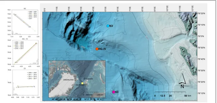
The stations of the HAUSGARTEN observatory are located in the Arctic at ca. 79◦ N along a latitudinal and bathymetric gradient, crossing the Fram Strait at water depths ranging between 250 and 5,500 m (Soltwedel et al., 2016). Previous assessments of litter covered the central station HG-IV (Bergmann and Klages, 2012; Figure 1) and the northern station N3 (Tekman et al., 2017). Here, images from the southernmost station S3 were analyzed to assess latitudinal differences of litter on the seafloor.
In addition, the time series of N3 and HG-IV were extended through the analysis of new footage. The stations N3 and HG- IV are ∼300–400 m deeper than S3, which is at ∼2,300 m depth. While N3 experiences the greatest sea ice coverage as it is located close to the marginal ice zone (MIZ), HG-IV is only subject to temporary ice coverage and S3 is ice-free in most years and characterized primarily by Atlantic water masses (Taylor et al., 2017). Overall, the expeditions to the Arctic have produced data on marine litter through photographic surveys conducted in 2002, 2004, 2007, and almost annually since 2011 (Supplementary Table S1).
Photographic Surveys and OFOS Specifications
All expeditions were undertaken in summer aboard the German research icebreaker RV Polarstern, except for 2013 when RV MS Merian was used, and HG-IV could not be surveyed due to ice conditions.
Marine litter was assessed through photographic surveys of the seafloor using a towed Ocean Floor Observation System (OFOS), which is equipped with a video and still camera. The steel frame currently carries four LED lights, an altimeter, telemetry, and three red laser pointers positioned 50 cm from each other to allow accurate area calculations and scaling of objects. The OFOS has been modified and improved over time.Supplementary Table S1 gives the specifications of all deployments for each expedition.
In 2002 and 2004, camera tracks were established at∼2,500 m water depth at HG-IV, N3, and S3. The OFOS has been towed at each station along the same linear track since the beginning of the time series to assess changes in epifaunal assemblages (Figure 1).
The transects were photographed for 4 h at 0.5–0.7 knots and a target altitude of 1.5 m, varying according to bottom topography and sea state. The images were triggered automatically every 20–
30 s depending on speed and manually when an item of interest occurred in the field of view.
Image Analysis
The images from each year and station were treated as individual samples to allow temporal and spatial comparisons. All images were analyzed using BIIGLE version 2.0 (Bio-Image Indexing and Graphical Labeling Environment), a web-based image annotation
FIGURE 1 |Location of the three stations and the HAUSGARTEN observatory and camera tracks at each site.
tool (Langenkämper et al., 2017). The same computer screen was used to avoid variation from differences in resolution at a zoom of 1× using BIIGLE’s lawnmower mode, which divides an image into 36 sub-sections and scrolls through each one of them to ensure complete analysis of the whole image.
For consistency with previous publications, every litter item observed was labeled and categorized according to a 13-material type classification similar to Mordecai et al. (2011), but rope and food waste were added (Table 1). Unidentifiable litter refers to items of non-mineral nor biological origin whose material could not be determined due to limitations in image resolution, but which was of anthropogenic origin judging by its color, shape, and size. Examples of the items from each category are included in Table 1. All images were screened
TABLE 1 |Categories of material types.
Material Example
Plastic Carrier bags, industrial packaging
Rubber Fragments
Styrofoam Polystyrene foam
Fisheries plastic Nets and fishing gear
Rope Synthetic cord
Glass Pieces of dark glass
Paper Wrapping paper
Metal Scrap
Timber Fragments of construction timbers
Food waste Fish carcass
Fabric Cloth
Pottery Fragments of ceramics
Unidentifiable litter (Unid.) Fragments of sharp and/or bright material
for putative litter items, followed by a second assessment to ensure correct categorization and even out learning effects. In a third run, all remaining objects were reviewed by 1–2 further experts to exclude objects of low certainty of origin and ensure comparability with Tekman et al. (2017) and Bergmann and Klages (2012). Poor-quality images and those that showed overlap with the previous image were excluded to avoid double counts.
The length of each litter item was measured using the BIIGLE rectangle tool. Items were then grouped into three size categories:
small (<10 cm), medium (10–50 cm), and large (>50 cm) (Bergmann and Klages, 2012). Epibenthic fauna interactions with litter were annotated aiming for the highest possible taxonomic resolution. The form of interaction was categorized as entangled, colonized by or “in contact with.” The three laser points in each image were detected automatically through a computer algorithm (Schoening et al., 2015), enabling calculation of the area covered by each image.
Data Processing
Data from Bergmann and Klages (2012) and Tekman et al.
(2017) were incorporated in the analysis to assess temporal and spatial trends in mean annual litter density, material, and size composition among and within years and stations, and at HAUSGARTEN observatory combining all three stations. The size composition of plastic items was analyzed to assess temporal and spatial trends. Litter count was converted to litter density according to:
LD= ni Ai
whereLD, litter density (items km−2);ni, litter count per image;
Ai, area of the image (km2).
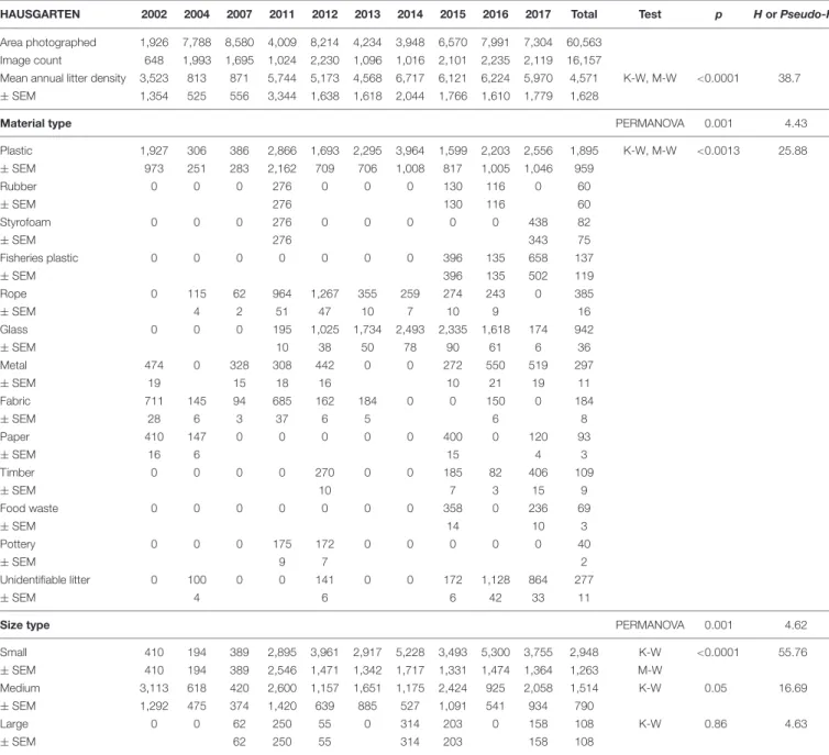
TABLE 2 |Summary of the area covered (m2), mean annual litter densities (items km−2), material and size composition at all HAUSGARTEN stations combined.
HAUSGARTEN 2002 2004 2007 2011 2012 2013 2014 2015 2016 2017 Total Test p HorPseudo-F
Area photographed 1,926 7,788 8,580 4,009 8,214 4,234 3,948 6,570 7,991 7,304 60,563 Image count 648 1,993 1,695 1,024 2,230 1,096 1,016 2,101 2,235 2,119 16,157
Mean annual litter density 3,523 813 871 5,744 5,173 4,568 6,717 6,121 6,224 5,970 4,571 K-W, M-W <0.0001 38.7
±SEM 1,354 525 556 3,344 1,638 1,618 2,044 1,766 1,610 1,779 1,628
Material type PERMANOVA 0.001 4.43
Plastic 1,927 306 386 2,866 1,693 2,295 3,964 1,599 2,203 2,556 1,895 K-W, M-W <0.0013 25.88
±SEM 973 251 283 2,162 709 706 1,008 817 1,005 1,046 959
Rubber 0 0 0 276 0 0 0 130 116 0 60
±SEM 276 130 116 60
Styrofoam 0 0 0 276 0 0 0 0 0 438 82
±SEM 276 343 75
Fisheries plastic 0 0 0 0 0 0 0 396 135 658 137
±SEM 396 135 502 119
Rope 0 115 62 964 1,267 355 259 274 243 0 385
±SEM 4 2 51 47 10 7 10 9 16
Glass 0 0 0 195 1,025 1,734 2,493 2,335 1,618 174 942
±SEM 10 38 50 78 90 61 6 36
Metal 474 0 328 308 442 0 0 272 550 519 297
±SEM 19 15 18 16 10 21 19 11
Fabric 711 145 94 685 162 184 0 0 150 0 184
±SEM 28 6 3 37 6 5 6 8
Paper 410 147 0 0 0 0 0 400 0 120 93
±SEM 16 6 15 4 3
Timber 0 0 0 0 270 0 0 185 82 406 109
±SEM 10 7 3 15 9
Food waste 0 0 0 0 0 0 0 358 0 236 69
±SEM 14 10 3
Pottery 0 0 0 175 172 0 0 0 0 0 40
±SEM 9 7 2
Unidentifiable litter 0 100 0 0 141 0 0 172 1,128 864 277
±SEM 4 6 6 42 33 11
Size type PERMANOVA 0.001 4.62
Small 410 194 389 2,895 3,961 2,917 5,228 3,493 5,300 3,755 2,948 K-W <0.0001 55.76
±SEM 410 194 389 2,546 1,471 1,342 1,717 1,331 1,474 1,364 1,263 M-W
Medium 3,113 618 420 2,600 1,157 1,651 1,175 2,424 925 2,058 1,514 K-W 0.05 16.69
±SEM 1,292 475 374 1,420 639 885 527 1,091 541 934 790
Large 0 0 62 250 55 0 314 203 0 158 108 K-W 0.86 4.63
±SEM 62 250 55 314 203 158 108
The dataset obtained was used to calculate the mean and standard error of the mean (SEM). The mean annual litter density was calculated as the sum of litter densities divided by the total number of images per year per station. The SEM was calculated based on the mean litter density of each transect per year. Out of the 13 material categories differentiated for statistical purposes, a summary of four categories (plastics, glass, other, unidentifiable litter) was used to illustrate the trends. The proportion of litter items that interacted with epibenthic megafauna was calculated and categorized as the percentage of items entangled, colonized or in contact with fauna. In addition, the interaction between megafauna and litter at the community and population level was determined for the most frequently affected species from 2004 to 2015. Epibenthic megafaunal density data obtained from the
same OFOS surveys were used to quantify the proportion of individuals affected by litter in every year at N3 and S3 (2004–
2015) and HG-IV (2002–2011) (Taylor et al., 2017; Bergmann et al., 2011). The number of interactions were presented as percentages of the mean count at the observatory. In the absence of reference data on megafaunal densities litter, data from 2016 to 2017 had to be excluded. The interaction at the population level refers to two species of sponges Cladorhiza gelida and Caulophacus arcticus, whose mean abundance was combined to assess sponge entanglement over time. The calculations were computed per station per year as follows:
(1) Number of individuals for litter study area = species density from literature×litter study area covered
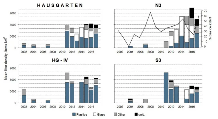
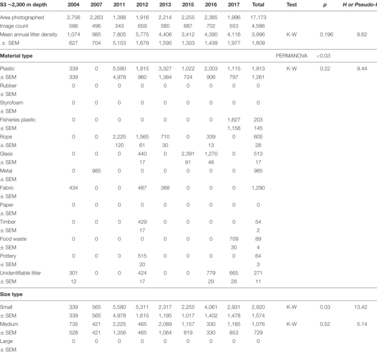
FIGURE 2 |Mean annual litter density and composition at HAUSGARTEN (all stations combined) and individual stations between 2002 and 2017. The percentage of summer sea ice extent is shown only at N3 highlighting the inverse trend during the last 3 years of the time series.
(2) Proportion of individuals affected by litter = Number of litter items
Number of individuals for litter study area
Statistical Analysis
The litter density data were tested for significant differences among years and stations by applying a Kruskal–Wallis test performed in MINITAB (version 14.12.0). When significant overall differences were found, pairwise Mann–Whitney U tests were conducted to assess, which years and stations were different.
A Bonferroni correction was applied to avoid Type-1 errors through multiple comparisons. This was done by dividing the p-value by the number of comparisons among years. For material and size composition, a one-way permutational multivariate analysis of variance (PERMANOVA) was performed in PRIMER (version 6.1.16) and PERMANOVA+(version 1.0.6) on a Bray Curtis similarity matrix. The data were 4th-root transformed to decrease an importance of dominant categories. Station was selected as a fixed factor to assess the differences in litter composition among stations and the effect of depth and ice coverage. Year was treated as a random factor since the surveys could not be conducted every year between 2002 and 2017 due to accessibility of the sampling site, availability of ship time and equipment. When significant differences were detected, a pairwise PERMANOVA was computed to assess, which years and stations were different. We included only those years in statistical comparisons, for which data were available at all stations.
Maritime Data and Summer Sea Ice Extent
Vessel monitoring system (VMS) reports were obtained from the Norwegian Directorate of Fisheries and used as a proxy of fishing activity inside the 12-nm area west of Svalbard. VMS data refer to vessel reports of time, position, course, and speed of EU fishing vessels longer than 24 m and foreign vessels longer than 15 m every 60 min. The number of reports was provided per country of origin (Russia, Norway, and Others) for each year from 2001 to 2017. In addition, the Harbormaster of Longyearbyen provided annual figures for the number of ships calling at the harbor of Longyearbyen. The ship calls were divided in tourism activities (cruises, coastal vessels, day-tour boats, and private yachts) and other-type-of-activities (cargo, research, fishing, governor’s vessels, navy, pilot boats). The number of passengers on tourism vessels were also analyzed for temporal trends. We tested for a correlation between all the maritime data and annual mean litter density at HAUSGARTEN (Spearman’s rank correlation, for all stations combined).
Daily sea-ice concentrations over the three stations were obtained from the Center for Satellite Exploitation and Research (CERSAT) at the Institut Français de Recherche pour l’
Exploitation de la Mer (IFREMER, France) (Ezraty et al., 2007) and ice coverage was calculated based on the ARTIST Sea Ice (ASI) algorithm developed at the University of Bremen, Germany (Spreen et al., 2008) at a 12.5×12.5 km resolution. Mean values for summer months (May–September) during the study period
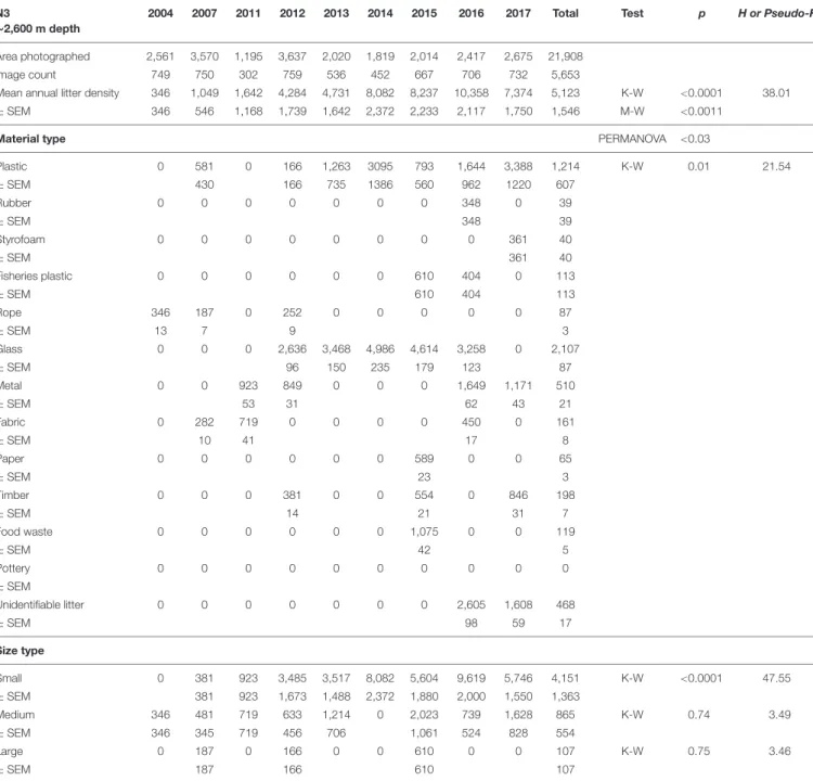
TABLE 3 |Summary of the area covered (m2), mean annual litter densities (items km−2), material and size composition at HAUSGARTEN station N3.
N3
∼2,600 m depth
2004 2007 2011 2012 2013 2014 2015 2016 2017 Total Test p H or Pseudo-F
Area photographed 2,561 3,570 1,195 3,637 2,020 1,819 2,014 2,417 2,675 21,908
Image count 749 750 302 759 536 452 667 706 732 5,653
Mean annual litter density 346 1,049 1,642 4,284 4,731 8,082 8,237 10,358 7,374 5,123 K-W <0.0001 38.01
±SEM 346 546 1,168 1,739 1,642 2,372 2,233 2,117 1,750 1,546 M-W <0.0011
Material type PERMANOVA <0.03
Plastic 0 581 0 166 1,263 3095 793 1,644 3,388 1,214 K-W 0.01 21.54
±SEM 430 166 735 1386 560 962 1220 607
Rubber 0 0 0 0 0 0 0 348 0 39
±SEM 348 39
Styrofoam 0 0 0 0 0 0 0 0 361 40
±SEM 361 40
Fisheries plastic 0 0 0 0 0 0 610 404 0 113
±SEM 610 404 113
Rope 346 187 0 252 0 0 0 0 0 87
±SEM 13 7 9 3
Glass 0 0 0 2,636 3,468 4,986 4,614 3,258 0 2,107
±SEM 96 150 235 179 123 87
Metal 0 0 923 849 0 0 0 1,649 1,171 510
±SEM 53 31 62 43 21
Fabric 0 282 719 0 0 0 0 450 0 161
±SEM 10 41 17 8
Paper 0 0 0 0 0 0 589 0 0 65
±SEM 23 3
Timber 0 0 0 381 0 0 554 0 846 198
±SEM 14 21 31 7
Food waste 0 0 0 0 0 0 1,075 0 0 119
±SEM 42 5
Pottery 0 0 0 0 0 0 0 0 0 0
±SEM
Unidentifiable litter 0 0 0 0 0 0 0 2,605 1,608 468
±SEM 98 59 17
Size type
Small 0 381 923 3,485 3,517 8,082 5,604 9,619 5,746 4,151 K-W <0.0001 47.55
±SEM 381 923 1,673 1,488 2,372 1,880 2,000 1,550 1,363
Medium 346 481 719 633 1,214 0 2,023 739 1,628 865 K-W 0.74 3.49
±SEM 346 345 719 456 706 1,061 524 828 554
Large 0 187 0 166 0 0 610 0 0 107 K-W 0.75 3.46
±SEM 187 166 610 107
were analyzed for Spearman’s rank correlation with mean litter densities at individual stations (Tekman et al., 2017).
RESULTS
Here, we present rare time-series data for litter in the deep Arctic sea and data on interactions with epibenthic megafauna at the population level. A total of 60.5 km2 were covered in 16,157 images for this study. The mean litter densities, at all HAUSGARTEN stations combined, ranged between 813±525 (SEM) and 6,717±2,044 (SEM) items km−2.
Temporal and Spatial Trends in Litter Density
Mean annual litter densities were significantly different over time (K-W: H = 38.7, df = 6,p<0.001) for all HAUSGARTEN stations combined. An initial strong increase in 2011 was followed by elevated levels above 6,000 items km−2from 2014 and thereafter (Table 2 andFigure 2). In terms of latitudinal differences, N3 was the most polluted station with the highest litter density recorded so far in 2016 (10,358 items km−2, Table 3). It was also the only station with a clear, continuous increase over time and significant differences among years (K-W: H = 38.01, df = 6, p<0.001). The year 2004 was significantly different from the
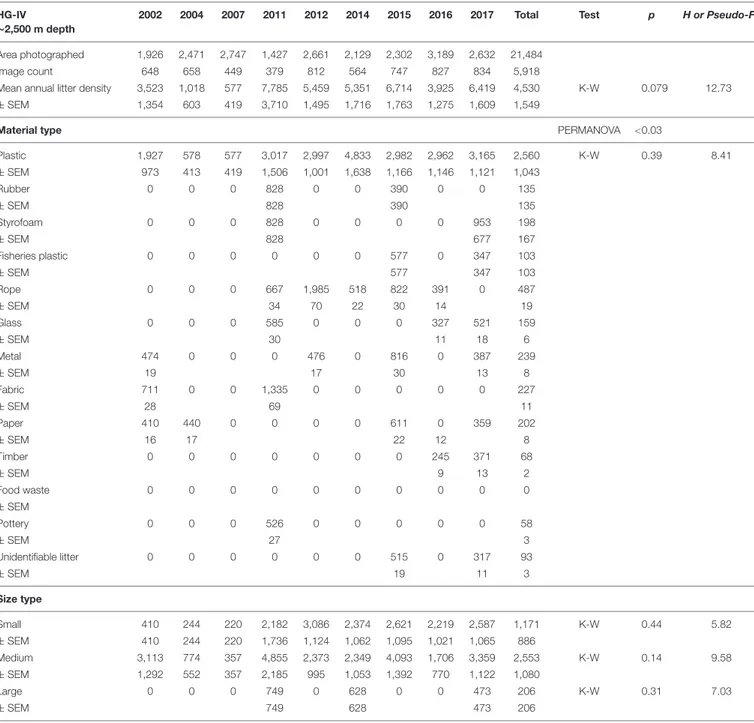
TABLE 4 |Summary of the area covered (m2), mean annual litter densities (items km−2), material and size composition at HAUSGARTEN station HG-IV.
HG-IV
∼2,500 m depth
2002 2004 2007 2011 2012 2014 2015 2016 2017 Total Test p H or Pseudo-F
Area photographed 1,926 2,471 2,747 1,427 2,661 2,129 2,302 3,189 2,632 21,484
Image count 648 658 449 379 812 564 747 827 834 5,918
Mean annual litter density 3,523 1,018 577 7,785 5,459 5,351 6,714 3,925 6,419 4,530 K-W 0.079 12.73
±SEM 1,354 603 419 3,710 1,495 1,716 1,763 1,275 1,609 1,549
Material type PERMANOVA <0.03
Plastic 1,927 578 577 3,017 2,997 4,833 2,982 2,962 3,165 2,560 K-W 0.39 8.41
±SEM 973 413 419 1,506 1,001 1,638 1,166 1,146 1,121 1,043
Rubber 0 0 0 828 0 0 390 0 0 135
±SEM 828 390 135
Styrofoam 0 0 0 828 0 0 0 0 953 198
±SEM 828 677 167
Fisheries plastic 0 0 0 0 0 0 577 0 347 103
±SEM 577 347 103
Rope 0 0 0 667 1,985 518 822 391 0 487
±SEM 34 70 22 30 14 19
Glass 0 0 0 585 0 0 0 327 521 159
±SEM 30 11 18 6
Metal 474 0 0 0 476 0 816 0 387 239
±SEM 19 17 30 13 8
Fabric 711 0 0 1,335 0 0 0 0 0 227
±SEM 28 69 11
Paper 410 440 0 0 0 0 611 0 359 202
±SEM 16 17 22 12 8
Timber 0 0 0 0 0 0 0 245 371 68
±SEM 9 13 2
Food waste 0 0 0 0 0 0 0 0 0 0
±SEM
Pottery 0 0 0 526 0 0 0 0 0 58
±SEM 27 3
Unidentifiable litter 0 0 0 0 0 0 515 0 317 93
±SEM 19 11 3
Size type
Small 410 244 220 2,182 3,086 2,374 2,621 2,219 2,587 1,171 K-W 0.44 5.82
±SEM 410 244 220 1,736 1,124 1,062 1,095 1,021 1,065 886
Medium 3,113 774 357 4,855 2,373 2,349 4,093 1,706 3,359 2,553 K-W 0.14 9.58
±SEM 1,292 552 357 2,185 995 1,053 1,392 770 1,122 1,080
Large 0 0 0 749 0 628 0 0 473 206 K-W 0.31 7.03
±SEM 749 628 473 206
years 2014 and thereafter (M-W:p<0.0011). Litter densities at HG-IV reached 7,785 items km−2in 2011 and remained elevated around 5,000 items km−2(Table 4) with no statistical differences (K-W: H = 12.73, df = 7, p = 0.079). At the southernmost station S3, litter densities peak in 2011 followed by a decrease but remained higher than in the early surveys (Table 5). There were no significant differences among years (K-W: H = 8.62, df = 6,p<0.196).
Trends in Material Composition
The composition of debris observed at HAUSGARTEN was significantly different throughout the years (PERMANOVA: Pseudo-F = 4.43, p = 0.001) with no clear
temporal trend (Figure 2). Plastic bags, packaging material and fishing gear were the most common form of plastic. This material accounted for 41% (Figure 2) at the observatory, with a significant boost after 2014 (K-W: H = 25.88, df = 8, p < 0.001). The second most frequent type were pieces of green glass (21%). Other material types such as metallic scrap, synthetic cord, timber, fragments of ceramics, and a probably discarded fish carcass accounted for less than 10% (Table 2).
There were significant differences in the litter composition of different stations (PERMANOVA:p<0.03). N3 held a distinct composition, where glass was the single most important material type (41%) while plastic accounted only for 24%. In contrast, HG-IV and S3 harbored mainly plastic, 77 and 49%, respectively.
TABLE 5 |Summary of the area covered (m2), mean litter densities (items km−2), material and size composition at HAUSGARTEN station S3.
S3∼2,300 m depth 2004 2007 2011 2012 2013 2015 2016 2017 Total Test p H or Pseudo-F
Area photographed 2,756 2,263 1,388 1,916 2,214 2,255 2,385 1,996 17,173
Image count 586 496 343 659 560 687 702 553 4,586
Mean annual litter density 1,074 985 7,805 5,775 4,406 3,412 4,390 4,116 3,996 K-W 0.196 8.62
± SEM 627 704 5,153 1,679 1,595 1,303 1,439 1,977 1,809
Material type PERMANOVA <0.03
Plastic 339 0 5,580 1,915 3,327 1,022 2,003 1,115 1,913 K-W 0.22 9.44
±SEM 339 4,978 960 1,384 724 906 797 1,261
Rubber 0 0 0 0 0 0 0 0 0
±SEM
Styrofoam 0 0 0 0 0 0 0 0 0
±SEM
Fisheries plastic 0 0 0 0 0 0 0 1,627 203
±SEM 1,158 145
Rope 0 0 2,225 1,565 710 0 339 0 605
±SEM 120 61 30 13 28
Glass 0 0 0 440 0 2,391 1,270 0 513
±SEM 17 91 48 17
Metal 0 985 0 0 0 0 0 0 985
±SEM
Fabric 434 0 0 487 368 0 0 0 1,290
±SEM
Paper 0 0 0 0 0 0 0 0 0
±SEM
Timber 0 0 0 429 0 0 0 0 54
±SEM 17 2
Food waste 0 0 0 0 0 0 0 709 89
±SEM 30 4
Pottery 0 0 0 515 0 0 0 0 64
±SEM 20 3
Unidentifiable litter 301 0 0 424 0 0 779 665 271
±SEM 12 17 29 28 11
Size type
Small 339 565 5,580 5,311 2,317 2,255 4,061 2,931 2,920 K-W 0.03 13.42
±SEM 339 565 4,978 1,615 1,195 1,017 1,402 1,478 1,574
Medium 735 421 2,225 465 2,089 1,157 330 1,185 1,076 K-W 0.52 5.14
±SEM 528 421 1,356 465 1,064 819 330 853 729
Large 0 0 0 0 0 0 0 0 0
±SEM
Temporal Trends in Litter Size Composition
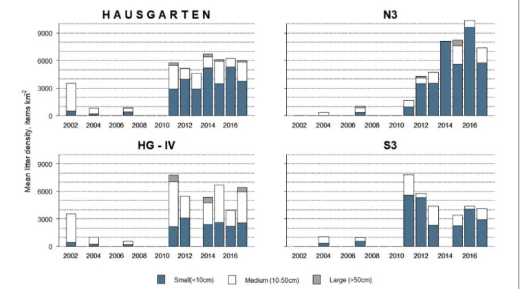
Overall, 63% of the litter was small whereas medium-sized items accounted for 35% and large items were scarce (2%). The size of litter varied significantly over time (PERMANOVA: Pseudo-F = 6.08, p = 0.001) with the quantity of small items increasing after 2011 (K-W, M-W:
H = 55.76,p<0.001). These dominated (>70%) at N3 and S3 (Figure 3) although there were no significant spatial differences (PERMANOVA:p>1.22).
Temporal Trends in Plastics Litter Size
Overall, a similar proportion of small and medium-sized plastics was observed at the observatory, 49 and 47%, respectively. Small plastics came mostly from HG-IV in 2013 and S3 in 2011.
Coincidentally, both stations harbored exclusively plastics in those years (Figure 2). Plastic is the main material type and comes mostly in small size, which raises concern about further fragmentation and microplastic pollution, especially because the quantity of small plastics continued to grow after the 2014 maximum (K-W, M-W: H = 25.88, df = 8, p<0.002).
FIGURE 3 |Size composition of litter observed at the HAUSGARTEN observatory and at each station in terms of mean annual litter density between 2002 and 2017.
FIGURE 4 |Examples of marine litter photographed by OFOS at HAUSGARTEN:(A)Styrofoam lying onCaulophacusdebris,(B)plastic film in contact with two Bythocarisshrimps,(C)Bythocarissp. resting on plastic bag,(D)plastic wrapping material entangled inC. arcticusand colonized byB. margaritacea,(E)fisheries plastics and probably food waste, which attracted scavenging amphipods and eelpout (Lycodes frigidus),(F)piece of rubber colonized by anemones,Verum striolatumand calcareous tube worm, (G) piece of plastic entangled inCladorhiza gelidaand colonized by sea anemones.
Litter Interaction With Epibenthic Megafauna
Overall, 45% of the litter items interacted with epibenthic fauna either by entanglement, colonization or by being “in contact”
(Figure 4). The most common material observed to encounter fauna was plastic (30%), other material types accounted for less than 5% each. The highest proportion of interactions was
recorded at HG-IV (66%) followed by N3 (22%), and S3 (12%).
Litter items interacted with 158 individuals of 12 taxa. Litter was frequently entangled in sponges, especially of the speciesC. gelida (26%).C. arcticus, another species of sponge, was also entangled regularly with litter (11%), its debris even more often (17%) with almost half of those interactions seen at N3. The second most common interaction entailed anemones colonizing litter,
FIGURE 5 |Proportion of the spongesCladorhiza gelidaandCaulophacus arcticusentangled with marine litter at N3 (white circles) and S3 (black triangles) between 2004 and 2015.
particularly of the family Hormathiidae (22%), well over half of these colonizations were observed at HG-IV. This form of interaction occurred with another anemone, Bathyphellia margaritacea(5%) and the sea lilyBathycrinus carpenterii(8%).
Other interactions (<4%) included crustaceans (Bythocarissp., Birsteiniamysis inermis), goose barnacles (Verum striolatum), soft corals (Gersemia fruticosa), other sponges (cf. Pachastrellidae) and sea cucumbers.
For the first time, we present figures on the proportion of epibenthic megafaunal organisms interacting with litter at HAUSGARTEN. The proportion of epibenthic megafaunal
organisms interacting with litter was low ranging between 1 and 31% with no clear temporal trend over time. When looking into populations of species, however, there was an increase in the number of sponges (C. gelida and C. arcticus) entangled with litter at N3, the highest percentage was observed in 2015 (10%) (Figure 5). At S3, the proportion of entangled sponges was even higher and remained elevated after an initial peak in entanglements in 2011 (20%). While a greater proportion of C. gelidasuffered from entanglement at N3 (up to 28%), at S3 most litter got entangled inC. arcticus(up to 31%).
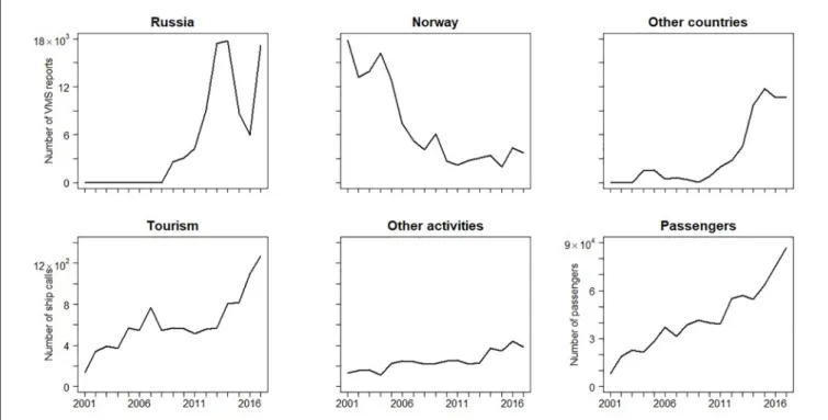
Maritime Traffic
The fishing activity from Russian vessels, inside the 12-nm range of Svalbard, was positively correlated with the overall litter density at HAUSGARTEN (ρ = 0.794,p = 0.006), where the number of VMS reports were particularly high in 2014 and 2017 (Figure 6). Likewise, vessels from other countries were positively correlated with litter densities (ρ = 0.656, p = 0.039) while there was no correlation with Norwegian vessels (ρ=−0.527,p= 0.117), probably because their numbers decreased over time.
The tourist ships calling at the port of Longyearbyen as well as the number of passengers, correlated positively with litter densities at HAUSGARTEN (ρ = 0.69, p = 0.025; ρ = 0.67, p= 0.033, respectively). Tourism and the number of passengers of leisure craft have steadily increased in the time frame of almost two decades. The latter reached 87,000 passengers per year in 2017 (Figure 6). When testing tourism ship categories individually, private yachts were most strongly correlated
FIGURE 6 |Temporal trend in the number of VMS reports from Russia, Norway, and other countries (upper panel, from left to right, source: Norwegian Directorate of Fisheries). Number of ships calling at the port of Longyearbyen (Svalbard) from tourism, other-type activities, and number of passengers of leisure craft (bottom panel, source: Harbormaster of Longyearbyen).
(ρ= 0.74,p= 0.013). However, the strongest correlations were found with other-type-of-activities ships (ρ= 0.85,p= 0.002), despite a low number of calls (<400 y−1).
Summer Sea Ice Extent
There was no correlation between the mean summer sea ice extent and litter density at any station (ρ > 0.08, p> 0.556).
Nonetheless, N3 experienced a reverse trend in sea ice coverage from 2015 to 2017: a decrease in sea ice cover coincided with an increase in litter density (Figure 2). As for the other two stations, HG-IV experienced a low sea ice coverage and S3 was ice-free except for the summers of 2007 and 2013.
DISCUSSION
Temporal Trends in Litter Density
This 15-year record of observations at HAUSGARTEN shows an increase in litter pollution over time with particularly high densities in 2011, 2014, and 2016. The deep seafloor is considered a sink for marine litter (Woodall et al., 2014) and as such, a particularly suitable environment for long-term observations.
However, although litter remained at an elevated level after the initial peak in 2011, there was no continuous increase across all years and stations concurring with results from other time-series studies (Law et al., 2010, 2014;Browne et al., 2015;Schulz et al., 2015; Nelms et al., 2017; Beer et al., 2018; Maes et al., 2018).
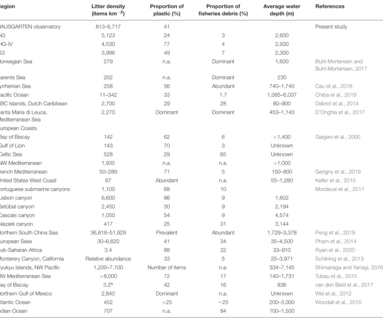
Table 6shows a comparison of litter densities and the proportion of plastics among studies on the deep seafloor. Most of the items recorded were only observed once and may have been eaten or moved by epibenthic organisms or bottom currents (on average 7.8 ± 0.9 cm s−1, Meyer-Kaiser et al., 2019). Fragmentation into smaller sizes including microplastics is another possibility although environmental conditions in the deep sea such as low temperatures, the absence of UV light and weak currents may slow down this process compared with other realms. In addition, litter items may have been hidden by a veneer of sediment over time. This suggests that litter densities at the observatory could be even higher. Assuming no transport and therefore a continuous accumulation of debris over time, cumulative litter densities could exceed our highest litter record tenfold (117,978 items km−2). Such densities have only been reported in the Mediterranean Sea (>100,000 items km−2), which has been considered the most polluted area in the world (CIESM, 2014).
Although sedimentation to the deep sea is a slow processBrandon et al. (2019)reported that (micro-)plastic pollution in sediments doubled every 15 years over a multidecadal time scale, showing an exponential increase over time and clearly indicating the burial of plastics in sediments.
The strong increase in litter in 2011 may be partly due to a switch to a new camera (Canon EOS-1Ds Mark III) fitted to the OFOS. This could potentially have increased object recognition although care was taken to include objects, which could only be identified with low certainty.
Plastic was the most frequent type of litter. This is not surprising given that plastic debris has spread to the abyss in various parts of the World’s Oceans (Debrot et al., 2014;
Pham et al., 2014; Woodall et al., 2014; Chiba et al., 2018;
Gerigny et al., 2019; Pierdomenico et al., 2019) even reaching its deepest parts, the hadal zone (Peng et al., 2018). Some of these locations bear exceptionally high mean densities, e.g., La Fonera (15,057 items km−2) and Cap de Creus canyons (8,090 items km−2) in the Mediterranean (Tubau et al., 2015), which are in a similar range with our highest records from N3 (10,358 items km−2). Unlike those places, however, the observatory is secluded from populated and industrial regions. Although, the largest proportion of litter in the Arctic originates most likely from long-distance transport from industrialized European and Atlantic destinations and drifts to the North via the thermohaline circulation (Cózar et al., 2017) our data show that the region is subject to increasing local shipping activity, especially in terms of tourist cruises and fishing. Shipping in the tourism sector increased to more than 1,000 ships per year in 2016 coinciding with a peak in litter densities recorded in that year. Similarly, the VMS reports of vessels from Russia grew to>17,000 in 2014 and from “other countries” to>10,000 in 2016, which may also have contributed to the peaks observed. These increases in shipping could be a response to the declining sea ice and changes in the ranges of fish stocks. Merchant shipping is likely to increase in the future as the Northern Sea route represents 50% of savings over the Asia to Europe via the Suez Canal route (Aksenov et al., 2017), and sea ice is likely to decrease further given rapidly rising greenhouse gas emissions enhancing global heating. Indeed, the high quantities of glass recorded at N3 point to local emissions.
Given its high density, glass can be assumed to sink to the seafloor directly. It should be noted that the disposal of glass in the Arctic was banned by MARPOL in 2013.
Material and Size Composition
Plastic materials have become a common feature of our oceans and the situation in the secluded Arctic is no exception. It accounted for 41% of the material observed on the seafloor, which is lower compared with the world’s average of ∼62%
on the seafloor (LITTERBASE, 2019). The global increase in plastic production has led to a cumulative plastic production of 8.3 billion MT in 2017 (Geyer et al., 2017). Along with its extensive usage, buoyancy capacity and durability (Andrady, 2015), the inefficient recycling and waste export schemes (Brooks et al., 2018) explain the subsequent mismanaged fraction that enters the ocean (Jambeck et al., 2015).
Positively buoyant items such as polyethylene and polypropylene, are commonly found in the surface layer and shorelines and can drift for extended periods of time. It is striking that some of these (fragments of) plastic items make it to the seafloor. This is often explained with a ballasting effect of fouling organisms (Fazey and Ryan, 2016), which reduces their original buoyancy. Still, the items in our images did not show any sign of the typical rafting biota (e.g., barnacles, mussels, hydroids, algal film). While fouling biota experience changes in temperature, pressure, and food supply during their passage to the seafloor likely leading to mortality, we think it is unlikely that their remains would fall off entirely. If this was the case, the buoyancy of such items may increase such that they could rise back to the sea surface unless they were entrapped by sediments,
TABLE 6 |Litter densities and plastic proportion of studies from the deep seafloor worldwide.
Region Litter density
(items km−2)
Proportion of plastic (%)
Proportion of fisheries debris (%)
Average water depth (m)
References
HAUSGARTEN observatory 813–6,717 41 Present study
N3 5,123 24 3 2,600
HG-IV 4,530 77 4 2,500
S3 3,996 49 7 2,300
Norwegian Sea 279 n.a. Dominant 1,600 Buhl-Mortensen and
Buhl-Mortensen, 2017
Barents Sea 202 n.a. Dominant 230
Tyrrhenian Sea 258 56 Abundant 740–1,740 Cau et al., 2018
Pacific Ocean 11–342 33 1.7 1,085–6,037 Chiba et al., 2018
ABC Islands, Dutch Caribbean 2,700 29 28 80–900 Debrot et al., 2014
Santa Maria di Leuca, Mediterranean Sea
2,270 Dominant Dominant 453–1,143 D’Onghia et al., 2017
European Coasts
Bay of Biscay 142 62 6 >1,400 Galgani et al., 2000
Gulf of Lion 143 70 3 Unknown
Celtic Sea 528 29 65 Unknown
NW Mediterranean 1,935 n.a. n.a. >1,000
French Mediterranean 50–289 71 5 150–800 Gerigny et al., 2019
United States West Coast 67 Abundant n.a. 55–1,280 Keller et al., 2010
Portuguese submarine canyons 1,100 68 10 Mordecai et al., 2011
Lisbon canyon 6,600 86 9 1,602
Setúbal canyon 2,450 30 9 2,194
Cascais canyon 1,050 54 9 4,574
Nazaré canyon 417 25 31 3,144
Northern South China Sea 36,818–51,929 Prevalent Abundant 1,729–3,378 Peng et al., 2019
European Seas 30–6,620 41 34 35–4,500 Pham et al., 2014
Sub-Saharan Africa 3.4 88 22 33–910 Ryan et al., 2020
Monterery Canyon, California Relative abundance 33 5 25–3,971 Schlining et al., 2013
Ryukyu Islands, NW Pacific 1,200–7,100 Number of items n.a. 334–7,145 Shimanaga and Yanagi, 2016
NW Mediterranean Sea >8,000 72 17 140–1,731 Tubau et al., 2015
Bay of Biscay 3.2a 42 16 836 van den Beld et al., 2017
Northern Gulf of Mexico 2,840 Dominant n.a. Unknown Wei et al., 2012
Atlantic Ocean 452 <25 ∼25 200–3,000 Woodall et al., 2015
Indian Ocean 707 n.a. 84 100–1,500
aDensity determined as number of items per 100 images. n.a., which means Not applicable.
stones, emergent fauna, or colonized by sessile benthic fauna.
Indeed, 30% of the plastic items were subject to such interactions.
Not only biofouling, but also hydrographic processes such as deep-water cascading and flash-flood events or eddies may promote downward transport (Lalande et al., 2011;Tubau et al., 2015;Pierdomenico et al., 2019).
As mentioned above, a large portion of glass (41%) was found at our northernmost station and to a lower extent at the other stations. This is important as it is an indicator of disposal from intensifying local maritime activity. Since glass is denser than seawater it immediately sinks. It is perceived as the least harmful material despite being very durable. Being a hard substratum, however, glass can be colonized by sessile biota and thereby alter local community structure and thus biodiversity in soft- sediment habitats.
Items smaller than 10 cm dominated at two out of the three stations (>50%), while the central station was characterized by
medium-sized items (>40%). However, almost a decade ago, medium-sized items were the frequent size at HAUSGARTEN (67%) (Bergmann and Klages, 2012). These temporal changes in size composition suggest fragmentation of plastics, the prime contributor of litter. Known to break down into smaller pieces, pollution from microplastics is also of great concern as these can be taken up by a wider range of biota. Indeed, HAUSGARTEN sediments harbored very high microplastic concentrations, with highest concentrations found at the northern station (6,595 and 13,331 particles kg sediment−1) (Bergmann et al., 2017c;
Tekman et al., 2020). A feedback mechanism with sea ice is suspected not only as a transport vehicle circling the Arctic basin but also as an accelerator of plastics fragmentation rates during subsequent melting and freezing seasons (Peeken et al., 2018; Tekman et al., 2020). Smaller plastics are more likely to sink due to a higher surface-to-volume ratio promoting ballasting through biofouling. In addition, small plastics can