The Arctic-Subarctic sea ice system is entering a seasonal regime: Implications for future Arctic amplification

Supplementary Information for:

The Arctic-Subarctic sea ice system is entering a seasonal regime: Implications for future Arctic amplification

Thomas W. N. Haine

and Torge Martin

1Earth & Planetary Sciences, The Johns Hopkins University, Baltimore, MD USA

2GEOMAR Helmholtz Centre for Ocean Research Kiel, Kiel, Germany

*Thomas.Haine@jhu.edu

+These authors contributed equally to this work.

ABSTRACT

Supplementary information on the seasonality number and supporting figures.

Discussion of Seasonality Number

Definition

Theseasonality number,Se(T), is defined by equation (1) of the main text. We consider a non-negative, time-dependent variablex(t)which is (quasi-)periodic, for example with a period of 12 months. The seasonality number is the ratio of two quantities, the seasonal range∆xin the variable for a given yearT,

∆x=x(t₂)−x(t₁), (SI1)

and the average value over the season,x, x= 1

t₂−t₁ Z t₂

t₁

x(t⁰)dt⁰. (SI2)

Namely,

Se(T) =|∆x|

x . (SI3)

In these formulaet₁andt₂are the times of consecutive extreme values ofx, typically separated by about six months. We take the absolute value in the numerator of (SI3) to suppress the negative sign ofSefor cases of seasonal decrease inx(when x(t₂)<x(t₁), which we apply throughout). The seasonality number is a function ofT because it can vary between successive pairs of extrema inx(t).

Pedagogical Examples

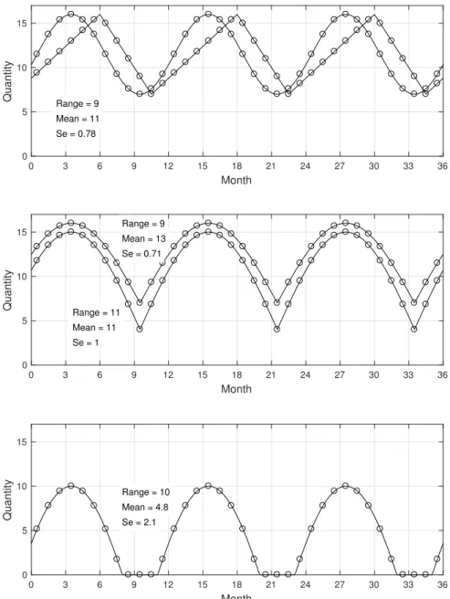
Consider the simple examples in FigureSI1to make the seasonality number concept clear. The upper two panels show annual periodic cycles with maxima and minima ofx(t₁) =16 andx(t₂) =7, and hence∆x=−9. They are inspired by the observed 1980s–1990s winter Arctic sea ice extent (16×10⁶km²) being about twice the summer extent (7×10⁶km²). The upper panel shows sinusoidal and sawtooth periodic functions. Although the times of their maxima and minima differ, they have identical ranges and mean values (x=11), so their seasonality numbers are the same and equal 0.78. These cases demonstrate the point thatSeis independent of the shape of the periodic functionx(t), so long as the range∆xand the meanxare unaffected. The middle panel shows a clipped sinusoidal function, also withx(t₁) =16,x(t₂) =7, and∆x=−9 (upper curve). This function accounts better for the different duration of the winter and summer seasons although still in a simplistic manner. The mean valuex=13 is larger than for the sinusoidal and sawtooth functions because the distribution ofxvalues over the year for the clipped sinusoid is biased towards higher values. Therefore, the seasonality numberSe=0.71 is smaller than for the upper panel. The middle panel also shows a clipped sinusoid function, but withx(t₁) =15,x(t₂) =4, hence∆x=−11, andx=11,

crudely resembling the Arctic sea ice extent cycle in recent years that features a stronger decline in summer than in winter. This case hasSe=1. The bottom panel shows a clipped sinusoid function that might resemble the Arctic sea ice extent cycle in the coming decades. In this case,x(t₁) =10,x(t₂) =0, hence∆x=−10, andx=4.8, yieldingSe=2.1. The distribution ofx values over the year is biased low compared to a sinusoid with the same range. Therefore the mean value is smaller thanx=5, which is the case for a sinusoid with the same range. Hence, the seasonality number is larger than for a sinusoid with the same range.

Properties of the Seasonality Number

These examples show that the seasonality numberSeis mainly controlled by the range∆x, and especially by the minimum value, not the mean valuex. Specifically, the middle panel of Fig.SI1shows an increase of 2 in∆x(lower curve) and ¯x(upper curve), compared to the upper panel. The∆xchange impactsSethree times more than the ¯xchange (a 28% increase versus a 9% decrease). The following arguments make this idea clear.

In many cases, the periodic function is evenly distributed between maxima and minima, meaning that the distribution ofx(t) betweenx(t₁)andx(t₂)is unbiased. Then,x= [x(t₂) +x(t₁)]/2, and the seasonality number for this unbiased seasonal cycle is

Se0(T) =2

|x(t₂)−x(t₁)|

x(t₂) +x(t₁)

=2

|ε−1|

ε+1

, (SI4)

whereε=x(t₂)/x(t₁). For the examples in Figure SI1, ε=7/16=0.438 (upper panel, upper curve on middle panel), 4/15=0.267 (lower curve on middle panel), and 0/10=0 (lower panel). Therefore, an unbiased seasonal cycle gives Se0=0.783, as seen for the sinusoid and sawtooth functions in the upper panel. The upper clipped sinusoid in the middle panel exhibits a bias that drivesxhigh and thereforeSe=0.71 is smaller than the value ofSe0=0.783 for the unbiased cycle, but still quite close. The lower clipped sinusoid in the middle panel is similar withSe₀=1.16 butSe=1. In the lower panel, the unbiased seasonal cycle givesSe₀=2, somewhat less than the actual value ofSe=2.1 because of the low bias inx(t).

This result shows thatSe>2 only occurs when there is a bias in the distribution ofx(t)so that the mean valuexis smaller than[x(t₂) +x(t₁)]/2. In other wordsSe₀≤2, which is seen in (SI4) because|ε−1|/(ε+1)≤1. For this reason, we refer to seasonality numbers greater than two as being in theepisodicregime (such as Fig.SI1lower panel), meaning thatx(t)only intermittently departs from near zero. There is no corresponding restriction on the smallness ofSein the perennial regime Se<1: as the range∆xdecreases for any minimumx(t)value greater than zero,Sealso decreases towards zero without limit.

Now consider that the mean valuexmust lie between the maximum and minimum values ofx(t);x(t₂)≤x≤x(t₁)(for ε<1, otherwise the inequalities are flipped). Therefore,

|1−ε| ≤Se(T)≤ 1 ε−1

(SI5) (forε<1, otherwise the inequalities flip). For the examples in the upper panel and upper curve in the middle panel of Figure SI1,ε=7/16=0.438 and therefore 0.563≤Se≤1.29, which is a moderately tight restriction on the seasonality number, regardless of the shape of the seasonal cyclex(t). For the lower panel, which shows anx(t)with a minimum value of zero, the seasonality number must satisfySe≥1, meaning anyx(t)with a minimum of zero cannot be in the perennial regime, regardless of the shape of its seasonal cycle. This is a reasonable property ofSe.

Notice that other putative definitions of the seasonality number, for example with the minimum value ofxin the denominator, not the average, have less desirable properties. In particular, if the denominator vanishes, as it does for Arctic sea ice in some of the CMIP5 models if the denominator is the minimum value, then the seasonality number diverges to infinity. That is less useful than the seasonality number defined by equation (1) of the main text, which naturally distinguishes between perennial, seasonal, and episodic regimes.

Relation between Sea Ice ExtentSeand Multi-Year Ice Extent

FigureSI2plots multi-year sea ice extentMY Iagainst seasonality numberSefor the data shown in Fig.1. Multi-year sea ice extent is defined as the minimum extent for a given year. As expected from the discussion above, there is a compact relationship betweenMY IandSe. The linear correlation coefficient for the northern hemisphere NSIDC data is -0.97, which shows that over the observational recordSeis strongly controlled byMY I(the line on Fig.SI2is the best-fit to these data). The southern hemisphere NSIDC data are offset to higherMY Ivalues (above the line). The same is true for the southern hemisphere HadISST data, although the scatter to largeMY IatSe≈1.25 is presumably due to data uncertainty before the satellite era. The CMIP5 models depart from the linear correlation atSe&1.3,MY I.2×10⁶km². At large seasonality number (Se&1.7 , MY I.1×10⁶km²), the multi-year ice extent no longer varies withSebecause it then depends mainly on the average extent (the denominator in equationSI3). Therefore,MY Iis a good proxy forSefor the Arctic over the observational record, and until the summer minimum sea ice extent drops below about 2×10⁶km².

Practical Considerations

A few practical issues should be considered when computing the seasonality number from a periodic time series. First, a clear idea of the period of interestt₂−t₁is required in order to avoid spurious extrema inxat shorter periods. For annually-repeating variables, we expectt₂−t₁to be close to six months, for example. Second, using the extreme values to define the range∆xof x(t)can be problematic when the time series contains significant random noise. Then, the extrema may be sensitive to the noise in undesirable ways. Although, this problem is unlikely to severely impact the computation of the seasonality number, it may be preferable to define∆xas the difference between (for example) the 95th and 5th percentiles of the distribution ofx(t)values between successive extrema. Third, for an annually-repeating variable one has the choice of defining the seasonality number each year based on the increase inx(t)(ε>1) or on the decrease inx(t)(ε<1). These two seasonality numbers may differ somewhat ifx(t)is biased differently for the increasing phase of its cycle compared to the decreasing phase.

Application to other Variables

The seasonality number is particularly useful for sea ice and can be applied to other Earth system quantities, such as insolation, ice mass, or heat content of the upper ocean. These are extensive (additive) quantities, which are non-negative by definition.

The seasonality number can be applied to intensive quantities too, but care is required. Specifically, it is not applicable to variables with an arbitrary offset. Temperature is a good example: it makes sense to talk of the seasonality number of absolute temperature measured in Kelvin (which is non-negative with a non-arbitrary zero), but not of temperature measured using an empirical scale such as Celsius or Fahrenheit.

0 3 6 9 12 15 18 21 24 27 30 33 36 Month

0 5 10 15

Quantity _{Range = 9}

Mean = 11 Se = 0.78 Range = 9 Mean = 11 Se = 0.78

0 3 6 9 12 15 18 21 24 27 30 33 36

Month 0

5 10 15

Quantity

Range = 9 Mean = 13 Se = 0.71

Range = 11 Mean = 11 Se = 1

0 3 6 9 12 15 18 21 24 27 30 33 36

Month 0

5 10 15

Quantity

Range = 10 Mean = 4.8 Se = 2.1

Figure SI1. Example annual periodic functionsx(t)and their seasonality numbersSeto illustrate the seasonality of Arctic sea ice extent. The range and mean are defined by equations (SI1) and (SI2), respectively, andSeis computed using (SI3).

0 0.5 1 1.5 2 2.5 Seasonality number, Se

0 2 4 6 8 10

Multi-year sea ice extent (x10 6 km 2 )

NSIDC Walsh et al.

HadISST PIOMAS CMIP5

Figure SI2. Multi-year sea ice extent plotted against seasonality number for the datasets shown in Fig.1. The large black dots are the pedagogical examples from Fig.SI1. The line is the best fit to the northern hemisphere NSIDC data.

5 10 15 20 25 30

Average sea ice volume (x10

km

)

5 10 15 20 25 30

Sea ice volume range (x10

km

)

5 10 15 20 25 30

Average sea ice extent (x10

km

) 5

10 15 20 25 30

Sea ice extent range (x10

km

)

0.3 0.6

1.0 1.4 1.8 2.2 3.0 4.0 Episodic

Seasonal

P e r e n n i a l

extent

volume

NSIDC PIOMAS

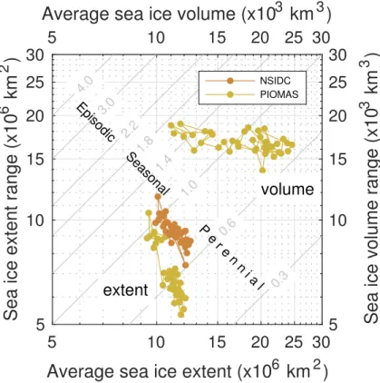
Figure SI3. Northern hemisphere seasonal sea ice extent (from NSIDC and PIOMAS) and volume (from PIOMAS) ranges plotted against the corresponding seasonal averages. The seasonality numbers are shown with contours. The sea ice extent and volume seasonality numbers increase with time (Figs.1b and2b), mainly because the ranges increase and the averages decrease, respectively.

1900 1950 2000 2050 2100 Year

0 10 20

Extent

ACCESS1-0

1900 1950 2000 2050 2100 Year

0 10 20

Extent

ACCESS1-3

1900 1950 2000 2050 2100 Year

0 10 20

Extent

BNU-ESM

1900 1950 2000 2050 2100 Year

0 10 20

Extent

CCSM4

1900 1950 2000 2050 2100 Year

0 10 20

Extent

CESM1-BGC

1900 1950 2000 2050 2100 Year

0 10 20

Extent

CESM1-CAM5

1900 1950 2000 2050 2100 Year

0 10 20

Extent

EC-EARTH

1900 1950 2000 2050 2100 Year

0 10 20

Extent

HadGEM2-AO

1900 1950 2000 2050 2100 Year

0 10 20

Extent

HadGEM2-CC

1900 1950 2000 2050 2100 Year

0 10 20

Extent

HadGEM2-ES

1900 1950 2000 2050 2100 Year

0 10 20

Extent

MIROC-ESM-CHEM

1900 1950 2000 2050 2100 Year

0 10 20

Extent

MIROC5

1900 1950 2000 2050 2100 Year

0 10 20

Extent

MIROC-ESM

1900 1950 2000 2050 2100 Year

0 10 20

Extent

MPI-ESM-LR

1900 1950 2000 2050 2100 Year

0 10 20

Extent

MPI-ESM-MR

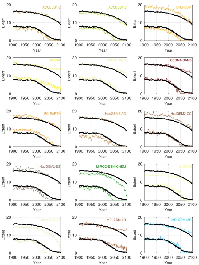
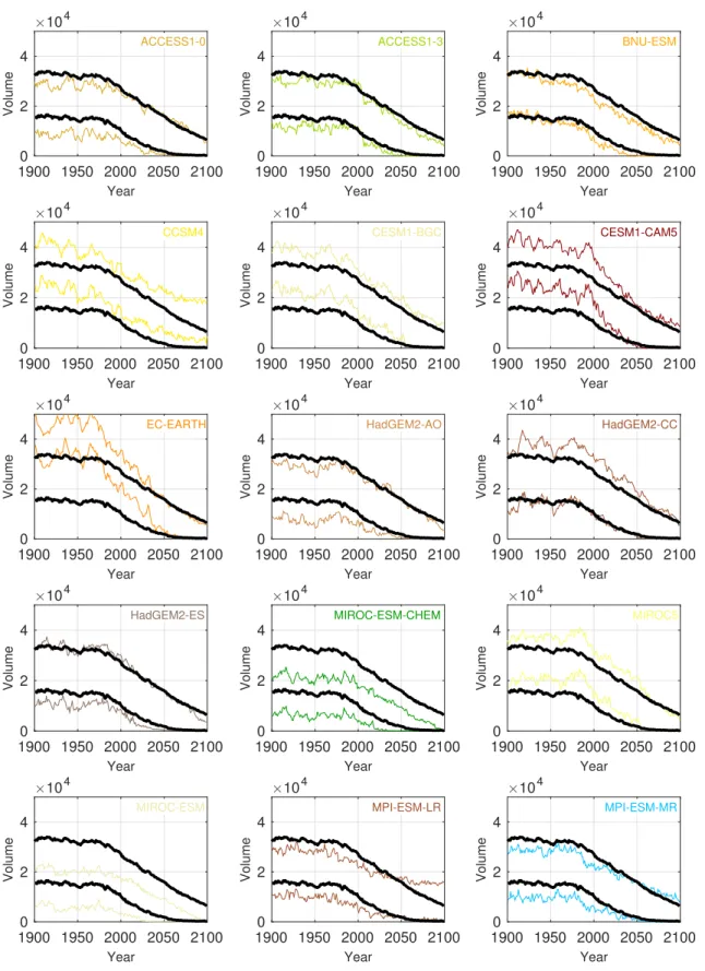
Figure SI4. Annual maxima and minima of sea ice extent for the CMIP5 models. The historical and RCP8.5 projections are shown. Black lines indicate the multi-model means.

1900 1950 2000 2050 2100 Year

0 2 4

Volume

10⁴

ACCESS1-0

1900 1950 2000 2050 2100 Year

0 2 4

Volume

10⁴

ACCESS1-3

1900 1950 2000 2050 2100 Year

0 2 4

Volume

10⁴

BNU-ESM

1900 1950 2000 2050 2100 Year

0 2 4

Volume

10⁴

CCSM4

1900 1950 2000 2050 2100 Year

0 2 4

Volume

10⁴

CESM1-BGC

1900 1950 2000 2050 2100 Year

0 2 4

Volume

10⁴

CESM1-CAM5

1900 1950 2000 2050 2100 Year

0 2 4

Volume

10⁴

EC-EARTH

1900 1950 2000 2050 2100 Year

0 2 4

Volume

10⁴

HadGEM2-AO

1900 1950 2000 2050 2100 Year

0 2 4

Volume

10⁴

HadGEM2-CC

1900 1950 2000 2050 2100 Year

0 2 4

Volume

10⁴

HadGEM2-ES

1900 1950 2000 2050 2100 Year

0 2 4

Volume

10⁴

MIROC-ESM-CHEM

1900 1950 2000 2050 2100 Year

0 2 4

Volume

10⁴

MIROC5

1900 1950 2000 2050 2100 Year

0 2 4

Volume

10⁴

MIROC-ESM

1900 1950 2000 2050 2100 Year

0 2 4

Volume

10⁴

MPI-ESM-LR

1900 1950 2000 2050 2100 Year

0 2 4

Volume

10⁴

MPI-ESM-MR

Figure SI5. As Fig.SI4except for sea ice volume.

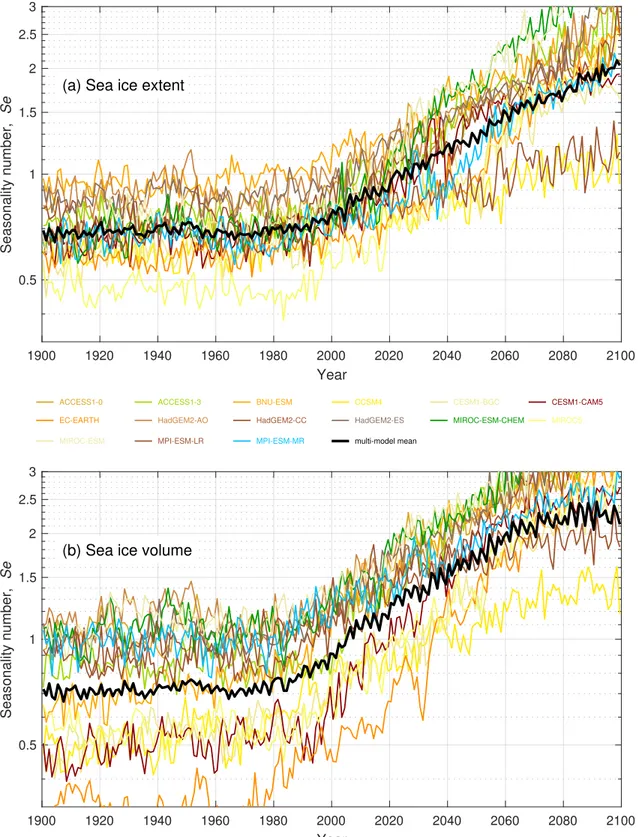
1900 1920 1940 1960 1980 2000 2020 2040 2060 2080 2100 Year

0.5 1 1.5 2 2.5 3

Seasonality number, Se

(a) Sea ice extent

1900 1920 1940 1960 1980 2000 2020 2040 2060 2080 2100

Year 0.5

1 1.5 2 2.5 3

Seasonality number, Se

(b) Sea ice volume

ACCESS1-0 ACCESS1-3 BNU-ESM CCSM4 CESM1-BGC CESM1-CAM5

EC-EARTH HadGEM2-AO HadGEM2-CC HadGEM2-ES MIROC-ESM-CHEM MIROC5

MIROC-ESM MPI-ESM-LR MPI-ESM-MR multi-model mean

Figure SI6. Seasonality of Arctic sea ice extent (upper) and volume (lower) for the CMIP5 models. The black line marks the multi-model mean.

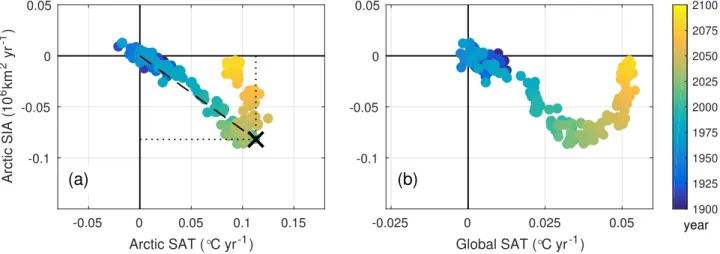
-0.05 0 0.05 0.1 0.15 Arctic SAT (°C yr^-1)

-0.1 -0.05 0 0.05

Arctic SIA (106 km2 yr-1 )

(a)

-0.025 0 0.025 0.05

Global SAT (°C yr^-1) -0.1

-0.05 0 0.05

year

(b)

1900 1925 1950 1975 2000 2025 2050 2075 2100

Figure SI7. Calculation of the peak in coincident sea-ice retreat and surface air temperature (SAT) warming. (a) Annual rate of change in Arctic (>70^oN) sea ice area (SIA) minimum as a function of the Arctic autumn (September to November) mean SAT annual rate of change (see Fig.4c). The black×marks the year with the largest normalized distance from the origin, namely, the largest change in both SIA and SAT, which we define as the peak in the sea ice feedback (see equation (2)). The SIA and SAT data are from the multi-model mean of the CMIP5 models. (b) Same as (a) but for global autumn mean SAT (notice the different abscissa scale).