Global and Planetary Change

(1)

Contents lists available atScienceDirect

Global and Planetary Change

journal homepage:www.elsevier.com/locate/gloplacha

Research article

Air-sea interactive forcing on phytoplankton productivity and community structure changes in the East China Sea during the Holocene

Zicheng Wang

^a,b

, Xiaotong Xiao

^a,b,⁎

, Zineng Yuan

^a

, Fei Wang

^a

, Lei Xing

^a

, Xun Gong

^c

, Yoshimi Kubota

^d

, Masao Uchida

^e

, Meixun Zhao

^a,b,⁎

aKey Laboratory of Marine Chemistry Theory and Technology, Ministry of Education, Institute for Advanced Ocean Study, Ocean University of China, Qingdao 266100, China

bLaboratory for Marine Ecology and Environmental Science, Qingdao National Laboratory for Marine Science and Technology, Qingdao 266237, China

cAlfred Wegener Institute, Helmholtz Centre for Polar and Marine Research, Am Alten Hafen 26, 27568 Bremerhaven, Germany

dNational Museum of Nature and Science, 4–1–1 Amakubo, Tsukuba City, Ibaraki 305–0005, Japan

eNational Institute for Environmental Studies, 16–2 Onogawa, Tsukuba, Ibaraki 305–8506, Japan

A R T I C L E I N F O

Keywords:

Biomarkers

Phytoplankton productivity and structure Kuroshio

East Asia Winter Monsoon Yellow Sea Warm Current

A B S T R A C T

Phytoplankton productivity and community structure in the East China Sea (ECS) play an important role in marine ecology and carbon cycle, but both have been changing rapidly in response to recent oceanic and at- mospheric circulation changes. However, the lack of long-term records of phytoplankton productivity and community structure variability in the region hinders our understanding of natural forcing mechanisms. Here, we use the phytoplankton biomarker (brassicasterol, dinosterol and alkenones) contents as well as the ratios between these biomarkers in three sediment cores from the ECS shelf to reconstruct the spatiotemporal variations of productivity and community of diatoms, dinoﬂagellates and coccolithophores during the Holocene, respectively. During 9–7 ka, the ECS shelf was characterized by low phytoplankton productivity with low coccolithophore contribution, caused by the oligotrophic condition mainly owing to the restricted Kuroshio Current (KC) intrusion under low sea-level conditions, thus the lack of nutrient input. Phytoplankton productivity generally increased during 7–4.6 ka, in response to the initial intrusion of the Yellow Sea Warm Current (YSWC, a branch of the KC), bringing nutrient from the subsurface KC to the upper layer of the ECS for phytoplankton growth. Phytoplankton productivity continuously increased during 4.6–1 ka, due to an enhanced circulation system (YSWC and Yellow Sea Coastal Current (YSCC)) driven by strong East Asia Winter Monsoon (EAWM).

Significantly, high alkenone contents and coccolithophore contribution in the eastern core F11A was associated with its location closer to the warm and saline YSWC, which was suitable for coccolithophore growth. Beyond diagenetic processes which could partly account for higher biomarker contents near core tops, elevated phytoplankton productivity during the last 1 ka might be induced by more nutrient supply from the intensified circulation system driven by enhanced KC and anthropogenic activities. The latter also resulted in high dinoflagellate proportions in all three cores. These temporal and spatial changes of phytoplankton productivity and community structure in the ECS during the Holocene corresponded to different mechanisms by the air-sea interaction, providing insights into distinguishing natural forcing and anthropogenic influences on marine ecology.

1. Introduction

Phytoplankton productivity and community structure play an important role in the global carbon cycle, regulating climate by controlling CO2level in the atmosphere (Chisholm, 2000;Rost and Riebesell, 2004;Schneider et al., 2008). As the basis of food web in the oceans, changes in phytoplankton productivity and community structure could

also influence the marine ecosystem (Cloern and Dufford, 2005). Phy- toplankton productivity is significantly related to sea surface nutrient concentration (cf. Chen, 2000). Since the industrial revolution, anthropogenic activities have led to increasing nutrient input, thus resulting in widespread coastal and marginal sea phytoplankton blooms, such as those during the 1980s and 1990s in the Aegean Sea and Black Sea (Moncheva et al., 2001), frequent red tides/harmful algal blooms

https://doi.org/10.1016/j.gloplacha.2019.05.008

Received 18 October 2018; Received in revised form 15 April 2019; Accepted 18 May 2019

⁎Corresponding authors at: Key Laboratory of Marine Chemistry Theory and Technology, Ministry of Education, Institute for Advanced Ocean Study, Ocean University of China, Qingdao 266100, China.

E-mail addresses:xtxiao@ouc.edu.cn(X. Xiao),maxzhao@ouc.edu.cn(M. Zhao).

Available online 23 May 2019

T

(2)

from 2002 to 2005 in the East China Sea (ECS) (Zhou et al., 2008) and the world's largest green tides in the summer of 2008 in the Yellow Sea (Liu et al., 2010a). Especially some toxic dinoflagellates are becoming dominant in the coastal habits of many countries, causing hypoxia in water column, significant fish kill and harming human health (Kirkpatrick et al., 2004;Walsh et al., 2006). However, recent studies reported that increased diatom productivity was a result of the increased natural forcing of upwelling in Zhejiang coastal area (Duan et al., 2014). Similarly, Florida red tides were also a natural phenom- enon caused by dense aggregations of unicellular organisms (Kirkpatrick et al., 2004). In order to understand mechanisms controlling phytoplankton blooms, it is essential to determine the spatial and temporal changes in phytoplankton productivity and community structure and their natural variability in the past.

Phytoplankton species such as diatoms and dinoflagellate/dinocysts in water column and surface sediments have been used to indicate the abundance of phytoplankton (cf. Chiang et al., 2004; Cho and Matsuoka, 2001). However, the use of diatom and dinoflagellate cyst for paleo-environment reconstruction was limited due to their poor preservation in marine sediments, e.g., dissolution of siliceous and carbonate frustule (Mudie et al., 2001). Biomarkers, fossil molecules, could be relatively well preserved in marine sediments and have been used to reconstruct long-term natural climate and ecological changes (Schubert et al., 1998;Werne et al., 2000;Zhao et al., 2006). Previous studies pointed out that lipid biomarkers in surface suspended particles can reflect relative phytoplankton biomass, as revealed by similar distribution patterns between lipid biomarkers and Chl a and/or phytoplankton cell counting (Sicre et al., 1994;Dong et al., 2012;Wu et al., 2016a). A recent study in the ECS also validated the applicability of brassicasterol, dinosterol, and C37alkenones as proxies of productivity and community structure of the three phytoplankton taxa: diatoms, dinoflagellates, and coccolithophores (Wu et al., 2016a). Therefore, community structures with relative contributions of diatoms, dinoflagellates and coccolithophores to phytoplankton productivity can be represented by brassicasterol/Sum (B/Sum, Sum =∑brassicasterol

+dinosterol+alkenones), dinosterol/Sum (D/Sum) and alkenones/

Sum (A/Sum), respectively (Schubert et al., 1998;Xing et al., 2016).

Brassicasterol/dinosterol ratio (B/D) is used to indicate the relative contribution of diatoms compared to dinoﬂagellates (Duan et al., 2014;

Xing et al., 2016). In the ECS, water mass properties (temperature, salinity, and inorganic nutrient) were important factors controlling phytoplankton biomass and community structure spatial variations (Wang and Cheng, 1988;Bi et al., 2018).

Today, primary productivity in the ECS is high with an average of 390–529 (mg C m²)/d (Ning et al., 1995;Gong et al., 2003), which has become an ideal area for environment and ecosystem change studies recently. When the Yellow Sea Warm Current (YSWC) intrudes on the ECS shelf as a branch of the Kuroshio Current (KC), the upwelling of the KC subsurface waters brings nutrients (especially phosphate and sili- cate) to the euphotic zone for phytoplankton growth (Chen, 2000;

Zhang et al., 2007). Thus, primary productivity of upwelling zones on the ECS continental slope is even higher than that of the terrestrial- nutrient-prevailing coastal areas (Chen, 2000). In addition, East Asia Winter Monsoon (EAWM) was reported as an essential driver of ecosystem changes in the ECS by driving the circulation system. In winter, the northerly EAWM drives the Yellow Sea Coastal Current (YSCC) and causes the pressure gradient along the Yellow Sea Trough, which forces the deeper northwestward intrusion of the YSWC as a compensating current of the YSCC (Yang, 2007; Xu et al., 2009; Yuan and Hsueh, 2010). Thus the intensiﬁed circulation system of the YSWC and the YSCC can induce the upwelling of nutrients to surface layer (Li et al., 2014and references therein), although the enhanced EAWM somehow might weaken the strength of the KC (Jian et al., 2000). Biomarker records reveal that the ecosystem change has been driven by both natural (Paciﬁc Decadal Oscillation) and anthropogenic forcing (terrestrial nutrient) over the last 100 years in the coastal areas of the ECS (Xing et al., 2016). However, lack of long-term and spatially-resolved records of phytoplankton productivity and community structure in the region hinders the understanding of ecosystem variation and its forcing mechanisms.

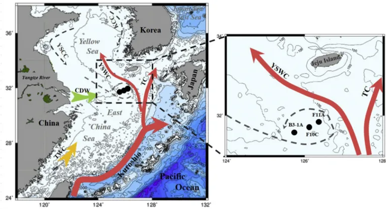
Fig. 1.A schematic map showing core sites (●) of B3-1A, F10C and F11A and regional circulation system in the ECS during winter. YSWC: Yellow Sea Warm Current;

TC: Tsushima Current; TWC: Taiwan Warm Current; YSCC: Yellow Sea Coastal Current; CDW: Changjiang Diluted Water; KCC: Korea Coastal Current.

Z. Wang, et al. Global and Planetary Change 179 (2019) 80–91

(3)

In this study, three sediment cores from the mud area on the ECS shelf with high sedimentation rate (Fig. 2) and relatively high organic carbon contents (average 0.7%) in surface sediments (Zhu et al., 2011), were used to reconstruct variations of phytoplankton productivity and community structure by multiple biomarker analyses. We compared the spatiotemporal variations of biomarker contents and their ratios to reveal the mechanisms controlling the phytoplankton productivity and community structure changes in the ECS during the Holocene, with the main focus on the air-sea interactive forcing.

2. Regional setting

The ECS, one of the largest shelf seas in the world, is located between the West Pacific and the East Asia Continent (Fig. 1). This region is influenced by both high-latitude climate forcing through the East Asian Monsoon and tropic-subtropical ocean circulation through the KC (Chen, 2009;Lie and Cho, 2016;Li et al., 2017). The East Asian Mon- soon results from the different potential heating between the West Pacific Warm Pool and the Asian continent, which is fundamental to climate dynamics over seasonal to millennial timescales (Webster et al., 1998;An, 2000). The Kuroshio is a western boundary current, serving as the returnflow for the wind-driven circulation of the North Pacific Subtropical Gyre. It transports large amounts of water, heat and materials, and has a significant influence on the climate and marine ecosystems in the vicinity of its path, including the ECS (Andres et al., 2008). The Kuroshio subsurface waters with enriched nutrients, at the depth of 70–220 m, upwell onto the slope and intrude on the ECS from the outer shelf to the inner area (Che and Zhang, 2018), contributing a large amount of nutrients to the ECS including our study sties. This contribution is many times more than the inputs from the Yangtze River and the Yellow River (Chen, 1996;Zhang et al., 2007). The YSWC is one of the most important dynamical phenomena in the ECS, and itflows northward along the Yellow Sea Trough. However, the formation process and forcing mechanisms of the YSWC are still controversial.Uda (1934) first described the YSWC as a branch of the Tsushima Warm Current originating from the KC, but later studies suggested that the YSWC was primarily forced by the pressure gradient induced by the northerly monsoonal winds (Yang, 2007;Yuan and Hsueh, 2010).Xu et al. (2009)used a 3-D Princeton Ocean Model to examine both the KC and monsoonal forcing on the variability of the YSWC and found the KC was responsible for most of the annual mean YSWC variations, while the local wind stress played an important but secondary role. Further- more, one upwelling center in the outer shelf of ECS associated with the cold eddy/front system was established around 6 ka (Xiang et al., 2008;

Xing et al., 2012;Yuan et al., 2018), caused by the anti-clock cyclone current due to the interaction between the YSWC and the YSCC (Hu

et al., 1980;Shen et al., 1993). Based on previous studies, the multi- year existence of the cold eddy/front system has been identiﬁed with thermal structure and current measurements (Mao et al., 1986) and its center is located around 31°30′N, 125°30′E with an inﬂuencing dia- meter of 100–200 km. The center could migrate due to the interaction between the YSWC and the YSCC (Fig. S3) (Shen et al., 1993;Wang et al., 2010).

3. Materials and methods 3.1. Sediment cores and age model

The three cores for this study were recovered from the ECS (Fig. 1), using a gravity sampler on R/V Dongfanghong 2 in 2011, F11A (31°53′

N, 126°21′E, water depth: 93 m, core length: 206 cm), F10C (31°45′N, 126°07′E, water depth: 65 m, core length: 205 cm) and B3-1A (31°37′ N, 125°45′E, water depth: 79 m, core length: 289 cm). All sediment samples were taken at 1 cm intervals and preserved frozen at−20 °C.

Benthic foraminifers from 7 depths of core B3-1A and from 5 depths of core F11A were picked for AMS¹⁴C dating at Peking University (Liu et al., 2007). For core F10C, three¹⁴C data points were acquired at AMS facility (NIES-TERRA), National Institute for Environmental Studies, Tsukuba, Japan (Uchida et al., 2004, 2008). All the measured AMS¹⁴C ages were calibrated to calendar ages using the CALIB 7.1.1 program and were corrected for a regional marine reservoir age (△R=−93 ± 69 yr.;Table 1).

3.2. Biomarker analysis

About 5 g freeze-dried sediment samples were ultrasonically extracted four times with 10 ml organic solvent (dichloromethane/MeOH 3:1, v/v) every time, after adding an internal standard (IS) mixture containing C19n-alcohol and C24deuterium-substitutedn-alkane. The extract was concentrated by gentle N2 stream, hydrolyzed with 6%

KOH-MeOH solution, and then extracted four times with 4 ml hexane on a vortex mixer. These extracts were further separated on silica gel chromatography being eluted by organic solvent. The hydrocarbon fraction (containingn-alkane) wasfirstly eluted with 8 ml hexane and the other fraction (containing alkenones and sterols) eluted with 12 ml dichloromethane/methanol (95:5,v/v). The fraction of alkenones and sterols was then dried under a gentle N2stream and derivatized using 0.04 mlN,O-bis(trimethylsilyl)-trifluoroacetamide (BSTFA) at 70 °C for 1 h before instrumental analysis. The identification of alkenones, brassicasterol and dinosterol was performed on a Thermo gas chro- matograph-mass spectrometer (GCMS), by comparing their mass spec- trum with those of their authentic standards, respectively, but the quantification of the biomarkers was performed on an Agilent 6890 N GC with an FID detector, using an HP-1 capillary column (50 m × 0.32 mm × 0.17μm) with hydrogen as a carrier gas at aflow rate of 1.3 ml/min. Oven temperature was kept initially at 80 °C for 1 min and then programmed to 200 °C at 25 °C/min, followed by 4 °C/

min to 250 °C, 1.7 °C/min to 300 °C (keeping for 10 min), andﬁnally 5 °C/min to 310 °C (keeping for 8 min). The content of each biomarker was calculated from ration of its GC peak integration to that of the IS.

The biomarker concentrations are reported as ng/g of bulk dry weight sediment.

Brassicasterol (B), dinosterol (D) and alkenone (A) are the cell membrane components of phytoplankton with diatom, dinoﬂagellate and coccolithophore being the main producers, respectively (Volkman, 1986), and to some extent their contents in marine sediments can re- ﬂect the corresponding phytoplankton biomass in the euphotic layer (Schubert et al., 1998;Werne et al., 2000;Zhao et al., 2006).

U37K'

values in core F10C were calculated based on the relative abundance of C37alkenones (Eq.(1)) (Prahl and Wakeham, 1987) and were converted into sea surface temperature (SST) using the global calibration (Eq.(2)) (Müller et al., 1998).

Table 1

Foraminifera¹⁴C data of cores B3-1A, F10C and F11A. All the measured AMS

14C ages were calibrated to calendar ages using the CALIB 7.1.1 program and were corrected for a regional marine reservoir age (△R=−93 ± 69 yr.).

Core Depth (cm) ¹⁴C age (¹⁴C yr. BP) SD ( ± yr.) Calendar age (yr. BP)

B3-1A 3 450 25 208

53 1675 30 1345

101 1975 25 1683

151 2380 25 2181

198 3015 20 2927

232 3485 20 3509

270 6660 25 7318

F10C 39 3750 30 3798

79 8440 40 9168

119 11,030 50 12,640

F11A 35 1065 25 734

81 1980 25 1690

124 2340 25 2121

164 3255 25 3258

204 4290 30 4584

(4)

⎜ ⎟

= ⎛

⎝ +

⎞

⎠

U ′ C

C C

37

K 37:2

37:2 37:3 (1)

= + = =

′ n

U₃₇^K 0.033SST 0.044, r 2 0.958, 370 (2)

where C37:2and C37:3indicated the C37alkenones with 2 and 3 double bonds, respectively.

U37K'

values of cores B3-1A and F11A were obtained fromYuan et al. (2018) and reconstructed SST data were recalculated by global equation (Müller et al., 1998).

4. Results 4.1. Chronology

The¹⁴C-dated core depths for B3-1A covered a time span of the last 9 ka. Linear interpolation between radiocarbon dates yielded sedimentation rates between 10 and 149.1 cm/kyr (Fig. 2A). The dated core interval for F11A spanned the Mid- and Late Holocene (4.6 ka) with sedimentation rates between 29.8 and 100.5 cm/kyr (Fig. 2C). For core F10C, the¹⁴C-dated covered a time span of the last 12.6 ka (Fig. 2B).

Linear interpolation between radiocarbon dates yielded sedimentation rates between 7.4 and 11.5 cm/kyr. The 2σerror bars for¹⁴C calendar ages are typically smaller than 300 years.

4.2. Biomarker contents

Brassicasterol contents in the three sediment cores had similar temporal trends, with a range of 25–390 ng/g in B3-1A, 8–237 ng/g in F10C and 103–627 ng/g in F11A. The contents in B3-1A and F10C were generally low during the Early Holocene and then increased in all the three sediment cores since 4.6 ka, with sharp increase from 1 ka to the top (Fig. 3).

The temporal trend of dinosterol was similar with that of brassicasterol in all three cores. Dinosterol contents were in a range of 36–818, 11–446 and 117–855 ng/g in B3-1A, F10C and F11A, respectively (Fig. 3).

Contents of alkenones here represent the sum of C37:2alkenone and C37:3alkenone. The temporal trends of alkenone contents were similar in B3-1A (10–203 ng/g) and F10C (0–151 ng/g), showing low values in B3-1A and zero values in F10C during the Early Holocene and increasing since about 4.6 ka (Fig. 3). The alkenone contents in F11A ﬂuctuated strongly in the whole record (19–414 ng/g) and were generally higher than those in B3-1A and F10C (Fig. 3).

The total biomarker contents showed an increasing trend in all three cores, in a range of 75–1398, 26–823 and 294–1563 ng/g in B3-1A, F10C and F11A, respectively (Fig. 3).

4.3. Biomarker ratios

B/Sum values in B3-1A (0.25–0.45) and F10C (0.28–0.47) generally increased during the Early Holocene and were relatively stable during 7–1 ka, and decreased during the last 1 ka (Fig. 4A, B, D and E).

However, B/Sum stronglyﬂuctuated in F11A, in the range of 0.26–0.46 (Fig. 4C and F).

D/Sum values were relatively stable in B3-1A (0.36–0.61) of the whole record, while decreased during the Early Holocene and increased since about 6 ka in F10C (0.40–0.68) (Fig. 4A, B, D and E). This ratio showed strongﬂuctuation in F11A, in the range of 0.27–0.56 (Fig. 4C and F).

A/Sum showed low values in B3-1A and F10C of the whole record, with the range of 0.07–0.35 and 0–0.23, respectively (Fig. 4A, B, D and E). However, A/Sum values were obvious higher in F11A (average 0.30 ± 0.11) than B3-1A (average 0.17 ± 0.05) and F10C (average 0.10 ± 0.07) (Fig. 4C and F; Table S1).

B/D values in B3-1A (0.39–1.05) and F10C (0.48–1.01) increased during the Early Holocene, were high during 7–1 ka and decreased since 1 ka (Fig. 4A, B, D and E). B/D values in F11A (0.57–1.39) were generally stable from 4.6 to 1 ka and decreased since 1 ka (Fig. 4C).

5. Discussion

5.1. Factors inﬂuencing sedimentary lipid biomarker contents

When using the lipid biomarkers for reconstruction of phytoplankton productivity and community structure, information of the source of phytoplankton biomarker is needed. According toVolkman et al. (1998), brassicasterol is not specifically derived from diatoms and is also abundant in some coccolithophores. In the ECS, diatoms and dinoflagellates are the dominant phytoplankton (Guo et al., 2014;Xiao et al., 2017), suggesting that the contribution of brassicasterol from coccolithophores could be minor. In addition, brassicasterol was found in a few species of dinoflagellates (Volkman, 2016), while a minor constituent of dinosterol was identified in a laboratory culture of a marine diatom Navicula sp. (Volkman et al., 1993). Surface water particulate sample studies suggest that, in diatom-dominated ecosystem such as upwelling regions and shelf seas, brassicasterol and dinosterol Fig. 2.Age-depth plots for cores B3-1A, F10C and F11A. Sedimentation rates were calculated using the calibrated ages of the dated horizons.

(5)

were likely mainly produced by diatoms and dinoﬂagellates respectively (Wu et al., 2016a). Thus, sedimentary biomarkers brassicasterol, dinosterol and alkenones in the ECS mainly originate from diatom, dinoﬂagellate and coccolithophore, respectively.

Beyond their production, the use of sedimentary lipids to reconstruct paleo-ecosystem must consider lipid diagenesis and lateral transportation that can inﬂuence lipid accumulation in sediments. First, diagenesis could cause rapid degradation of the organic compounds in the uppermost few centimeters of sediment cores (Canuel and Martens, 1996). Thus, the resultant rapid decrease of biomarker concentrations from the coretop to a few centimeters downcore was observed in all three cores in this study (Fig. 3). However, in the biomarker records of the long sediment cores from the ECS (Yuan et al., 2013; Wu et al., 2018), distinct high amplitude downcore variabilities were determined in the biomarker concentrations. Similarly, much higher amplitude of alkenones in core F11A than those in the other cores was observed in the current study, as alkenones in this site was more inﬂuenced by the variations of the YSWC. Our results indicate that changes in climate and marine environment were more likely to control the variability of biomarker contents rather than diagenetic processes in these sites.

Furthermore, proxies based on biomarker ratios such as B/Sum, D/Sum, A/Sum and B/D are less aﬀected by the diagenesis process in the ECS (Xing et al., 2016), although the degradation rates of these biomarkers are diﬀerent (Versteegh and Zonneveld, 2002;Wakeham et al., 2002).

Lateral advection by currents may alter sedimentary lipid biomarker contents at the sea floor (see Zonneveld et al., 2010and references therein). In this study, both individual and total biomarker contents in the middle core F10C were lower than those in the western and eastern cores during all time intervals (Figs. 3and S1), as the deposition of the sedimentary biomarkers in the three cores were influenced by the submarine topography (illustrated inFig. 6). The biomarkers produced in sea surface sink to seafloor at core site of F10C, and then might be laterally transported to neighboring locations of core B3-1A and core F11A because the water depth of core F10C was lower than the two neighboring cores (Fig. 6), resulting in obviously lower accumulation at F10C than those at B3-1A and F11A (Fig. 2).

5.2. Phytoplankton productivity and community structure during the Holocene

Several factors, such as nutrient, temperature and salinity, control the phytoplankton productivity and community structure in marine environment. Previous studies indicated that diatoms beneﬁted from high nutrient and dominated where chlorophyllawas high (Matsumoto et al., 2004; Takeda et al., 2007). For example, high abundance of diatoms was observed in the regions with high primary productivity in the ECS (Furuya et al., 2003). Dinoﬂagellate growth is also sensitive to phosphate concentrations and could also dominate under eutrophic conditions (Winder and Sommer, 2012; Ding et al., 2019), whereas coccolithophores could thrive under high-salinity, lower nutrient and warm water environments (Werne et al., 2000;Falkowski and Oliver, 2007). As the major coccolithophorid species in open ocean and marginal seas,E. huxleyihas not been reported in seawater with salinities below 11 psu (van der Meer et al., 2008), and coccolithophorid fossils were rarely found in sediments beneath lower salinity waters from the coast to the 50 m bathymetric line of the ECS, but they were common in deeper and higher salinity water sediments (Wang and Cheng, 1988).

Nevertheless, phytoplankton productivity is mainly controlled by the nutrient concentrations in the surface water from the temperate region (Chen, 2000; Xiao et al., 2017), but coccolithophore growth is ad- ditionally inﬂuenced by salinity changes (Saruwatari et al., 2016).

In this study, the time span of the three cores is different. The records of B3-1A and F10C covered the past 9 kyr while those for F11A covered only 4.6 kyr. A collective assessment of the three-core records would reveal that phytoplankton productivity was low during 9–7 ka, increased during 7–1 ka and reached high phases during 1–0 ka, respectively. The phytoplankton productivity changes during the interval 7–1 ka were likely caused by two different mechanisms before and after 4.6 ka (Fig. 6). Within the chronological uncertainties of cores, the 4.6 ka boundary may be related to the onset of Meghalaya (4.2–0 ka) as a new time period of Holocene (Walker et al., 2012). In the following sections, we described the temporal variability and spatial differences of the phytoplankton productivity and community structure in the ECS during the Holocene, and further discussed the possible climatic and Fig. 3.Variations of the biomarkers contents of B3-1A, F10C and F11A, respectively. B refers to brassicasterol, D refers to dinosterol and A refers to alkenones. Sum means the total contents of brassicasterol, dinosterol and alkenones.

(6)

oceanic forcing for each interval.

5.2.1. Low phytoplankton productivity and low coccolithophore contribution during the Early Holocene (9–7 ka)

Phytoplankton productivity was low in the ECS during the Early Holocene revealed by low biomarker contents in sediment cores B3-1A and F10C (Fig. 3), caused by oligotrophic conditions associated with the sea level changes (Fig. 6A). Sea level began to rise since the last deglacial as a result of warming and ice sheet melting (Xiang et al., 2007;Li et al., 2009;Shi et al., 2014, 2016). However, sea level was still about 17 m lower at 9 ka and gradually reached the present position at about 7 ka (Liu, 2001; Chough et al., 2004; Liu et al., 2004). This shallower marine environment could constrain the geographical space and pathways for the intrusion of the KC to the ECS shelf during the Early Holocene (Li et al., 2000), although the strength of the KC evi- dently reinforced, synchronous with a rapid sea level rise (Liu et al., 2004;Xiang et al., 2007). Therefore, this scenario limited the nutrient supply from the KC to the ECS shelf (Li et al., 2009), and consequently resulting in low phytoplankton productivity. Although the terrestrial organic matters to the ECS shelf were high due to the low sea level (Yuan et al., 2013), these terrestrial matters were most likely sourced from the reworked and re-suspended sediments of the ECS shelf but not from the riverine supply, inferred from the grain size and rare earth

elements study (Hu et al., 2014). Thus, nutrient from the terrestrial sources might have minor inﬂuence on phytoplankton growth during this time interval. Similarly, the biomarker records in the adjacent Yellow Sea also indicated low phytoplankton productivity during the Early Holocene due to low nutrient supply (Fig. 5;Wu et al., 2016b).

Although both diatom and dinoﬂagellate productivities were low (Fig. 3), their contributions during 9–7 ka were above the average values of the record (Table. S1). The relative contribution of dino- ﬂagellates was at maximum at such oligotrophic conditions, revealed by D/Sum and B/D values (Figs. 4 and 6; Table S1;Xing et al., 2012).

Notably, alkenone contents were below detection limit in core F10C during most of the Early Holocene (Fig. 3). Although coccolithophores with smaller cells are more competitive and thus can usually out- compete diatoms in oligotrophic environments (Kinkel et al., 2000;

Furuya et al., 2003; Baumann et al., 2005), their growth could be limited by salinity as the ECS was characterized by shallow marine environment with low salinity during this time interval because the YSWC had not formed yet (Kim and Kucera, 2000;Liu et al., 2010b;Mei et al., 2016). Similarly, the lower salinity stage during the Early Ho- locene has also been recognized in the adjacent southern Yellow Sea (Xiang et al., 2008) and in the middle Okinawa (Yu et al., 2009) based on benthic foraminiferal and stable isotope evidence. The formation of calcium carbonate shells of coccolithophores is closely related to the Fig. 4.Variations of the biomarker ratios and SST of B3-1A, F10C and F11A. B/Sum refers to the ratio between brassicasterol content and total biomarker content, D/

Sum refers to the ratio between dinosterol content and total biomarker content, and A/Sum refers to the ratio between alkenone content and total biomarker content.

SST records from cores B3-1A and F11A were modiﬁed fromYuan et al. (2018).

(7)

concentration of HCO3–in the seawater, thus low salinity is unfavorable for the its growth (Wang and Cheng, 1988;Saruwatari et al., 2016).

These interpretations of the Early Holocene records are supported by biomarker data in surface sediments and suspended particles from the continental shelf region of the ECS, which also reported that coccolithophores rarely contributed to the phytoplankton productivity in the shallower water environments (Ding et al., 2007). Furthermore, the changes in the content of C37 alkenones have been recently used to reﬂect the change in seawater salinity of the south Yellow Sea and to further track the formation and evolution of the YSWC on a long time scale (Mei et al., 2016).

5.2.2. Increased phytoplankton productivity and spatial variations of community structure during 7–1 ka

During 7–1 ka, phytoplankton productivity gradually increased on the ECS shelf, inferred by increased individual and total biomarker contents in the three cores, except the high andﬂuctuating alkenone contents in the eastern core F11A (Fig. 3). In the adjacent Yellow Sea, phytoplankton productivity was also enhanced since the Mid-Holocene, corresponding to increased nutrient supply (Kong et al., 2006; Zhao

et al., 2013;Wu et al., 2016b). However, diﬀerent mechanisms were applied to interpret the temporal variability and spatial diﬀerence of phytoplankton productivity and community structure on the ECS shelf during this time interval.

At the onset of this interval of 7–4.6 ka, phytoplankton productivity and community structure were mainly inﬂuenced by the initial formation of circulation system in the ECS. There is a consensus that the YSWC was formed around 6–7 ka, a period of high sea level that was close to the modern sea level (Kim and Kucera, 2000;Liu et al., 2008, 2010b). Sea level was 2–3 m higher than that of the present day during 7–6 ka, the KC reached its highest stage and the YSWC started to appear as a branch of the KC (Jian and Chang, 1999;Li et al., 2007, 2009), bringing nutrients from the subsurface KC water to the ECS surface for phytoplankton growth. Finally, modern pattern of the YSWC was established at about 5.5 ka inferred by the SST and salinity records in the adjacent Yellow Sea (Nan et al., 2017), triggering the formation of circulation system (YSWC and YSCC), consequently generating a cold eddy which upwelled nutrient to the eutrophic zone (Xiang et al., 2008;

Yuan et al., 2018). Therefore, the intrusion of the KC water to the ECS and the formation of the YSWC gradually strengthened from 7 to 4.6 ka Fig. 5.Comparison of phytoplankton productivity (Sum, ZY3 data obtained fromWu et al., 2016b), A/Sum and SST reconstructed in B3-1A, F10C and F11A, and KC index (Jian et al., 2000), EAWM index (Yancheva et al., 2007), ENSO index (Moy et al., 2002), sea level (Liu, 2001;Chough et al., 2004;Liu et al., 2004).

(8)

(Fig. 6B).

Phytoplankton community structure patterns were quite similar in core B3-1A and F10C during 7–4.6 ka, with increased contribution of coccolithophores (Fig. 4), although the alkenones concentrations were still low (Fig. 3). Salinity of the ECS increased signiﬁcantly after the formation of the Holocene YSWC (Liu et al., 2004). At the onset of the circulation system formation, intrusion of the saline and warm KC water could favor the coccolithophore growth (Kinkel et al., 2000;

Furuya et al., 2003;Baumann et al., 2005), although the circulation was still weak and the salinity was lower than modern (Xiang et al., 2008;

Xing et al., 2012; Fig. 6b). Relative contributions of diatoms and dinoflagellates were similar in western and middle cores (Fig. 4), although the spatial productivity is different (Fig. 3). This could be interpreted that both SSTs (23-25 °C) and nutrients were suitable for diatom and dinoflagellates growth (Anderson, 2000;Wang et al., 2006;

Chen, 2015;Xiao et al., 2017), although coccolithophores were also not limited at this temperature range.

Enhanced EAWM was likely the main factor for the continuously increasing phytoplankton productivity during 4.6–1 ka as the influences of the KC were reduced. Strong EAWM since around 4 ka was consistent Fig. 6.The schematic illustration of the variations of the phytoplankton productivity and community structure in the ECS during the Holocene. In the left-hand maps, black dots represent core sites as shown inFig. 1, red dotted circle represent for the expansion of cold eddy and the red solid circle represented for the cold eddy center. The black lines in (A) and (B) mean coastlines. In the right-hand maps, the circle size represents the relative contribution of phytoplankton productivity and the different colours represent the community structure. Red shade represents diatoms contribution, green shade represents dinoflagellates contribution and black shade represents coccolithophores contribution. (For interpretation of the references to colour in thisfigure legend, the reader is referred to the web version of this article.)

(9)

with the newly defined 4.2 ka event (onset of Meghalayan; Walker et al., 2012), marked by climate changes of cooling and aridity which caused cultural collapse in many places around world. This was also in agreement with decreased SSTs for several decades in our records (Fig. 4). The weakening of the KC during 4.6–2.7 ka was indicated by an abrupt decrease of the KC-associated foraminiferaP. obliquiloculatain the sediment cores on the pathway of the KC and its branches, caused by intensified EAWM (Fig. 6C) (Jian et al., 2000;Liu et al., 2013;Li et al., 2015). On the other hand, intensified EAWM enhanced the influence of coastal water with rich nutrient to the ECS shelf (Jian et al., 2000;Li et al., 2009). Contemporaneously, the circulation system was also further strengthened as intensified EAWM could drive the YSCC.

Similarly, previous studies confirmed the stable and continuous influence of the YSWC during the Mid-Holocene in both the Yellow Sea and the ECS (Liu et al., 2010a, 2010b;Nan et al., 2017). The steady circulation maintained the upwelling area, which supplied nutrient to the upper layer for phytoplankton growth. Notably, both individual and total phytoplankton productivities were higher in the eastern core F11A than those in the other two cores, especially the alkenone contents were significantly higher (Fig. 3). This could be interpreted that core F11A was much closer to the pathway of YSWC, benefiting from the nutrient brought by upwelling from the subsurface of the KC (Chen, 1996). Si- milarly, a modern study in the mud area of the ECS found that C37

alkenone concentrations in suspended materials were high in the east and very low in the west of the study area, with an obvious chlorophyll- a boundary along about 126°E (close to the middle core position of this study) (Ko et al., 2018). In addition, high salinity of YSWC water fa- vored coccolithophore growth in core F11A (Xing et al., 2011; Mei et al., 2016), thus resulting in very high alkenone contents (Fig. 3).

Spatial variation of individual phytoplankton productivity among the three cores indicated that coccolithophore growth is more sensitive to salinity changes than diatom and dinoﬂagellates (Xing et al., 2011).

Phytoplankton community structure in core B3-1A and F10C during 4.6–1 ka was similar with that during the previous stage 7–4.6 ka (Fig. 4). In contrast, coccolithophore contribution was significantly higher in F11A than those in western and middle cores during 4.6–1 ka (Fig. 4; Table S1), in agreement with a previous study from the Yellow Sea that the phytoplankton community structure had been characterized with increased coccolithophore contributions since the Mid-Holo- cene in response to the influence of YSWC (Xing et al., 2012). This spatial variation of community structure can be interpreted as more influence of high-temperature and saline YSWC on core site F11A than B3-1A and F10C as described above. The alkenone contents as well as the coccolithophore contributions in F11A during 4.6–1 ka were dis- tinctly higher than those in the other two cores although there were some low contents intervals (Figs. 3 and 4).

5.2.3. High phytoplankton productivity and community structure change between diatom and dinoﬂagellate (1–0 ka)

After 1 ka, phytoplankton productivity reached the highest level indicated by sharply elevated individual and total biomarker contents (Fig. 3). As discussed Section 5.1 above, the rapid increasing trend of biomarker contents near the core-top might be created by the diagenesis process, but we propose that productivity increases were the main cause, by considering both biomarker content and temperature records.

Biomarker records in the adjacent Yellow Sea also revealed a signiﬁcant increase in phytoplankton productivity during the Late Holocene, which was linked to the enhanced YSWC (Zhao et al., 2013). During this time interval, the KC was further enhanced, associated with decreased frequency of El Nino-South Oscillation (ENSO) events during the shift to La Nina mode (Fig. 5;Zheng et al., 2016). Low frequency of ENSO events could lead to the bifurcation of the North Equatorial Current occurring at a lower latitude and then resulting in a stronger KC (Hu et al., 2015 and references therein). Therefore, the YSWC was strengthened as a branch of the KC, in agreement with records in the ECS and Yellow Sea (Li et al., 2009). Consequently, the cold eddy was

strengthened in the ECS during the past 1 ka (Yuan et al., 2018), in agreement with modern observation that the ECS cold eddy was strengthened when the YSWC was strong (Chen et al., 2004;Hao et al., 2017), which could drive the upwelling nutrient to favor phytoplankton productivity and cool the SST (Figs. 4 and 6D). The elevated productivity in anticyclonic eddies has also been reported due to eddy- Ekman pumping in recent studies (He et al., 2016, 2017). Coincidently, the SST records in all three cores showed decreasing trend in response to the strengthened cold eddy (Fig. 5;Yuan et al., 2018). At core site F11A closer to the cold-eddy center, influence of the cold eddy might compensate the benefit to coccolithophores induced by the intensified YSWC, resulting in comparable alkenone contents during the Late Ho- locene to those during the previous stage (Fig. 4). In addition, the increased phytoplankton productivity during this interval was also pos- sibly linked to the gradually increasing anthropogenic influences.

Previous studies indicated that human activities in the upper and middle Changjiang have eﬀectively increased the Changjiang sediment load from about 240 to about 480 Mt./yr after 1 ka (Hori et al., 2001;

Wang et al., 2011).

Phytoplankton community structure change represented by biomarker ratios was generally similar in cores B3-1A and F10C during 1–0 ka (Fig. 4). The relative contribution of coccolithophores decreased in all three cores, however, it was still higher in core F11A than that in cores B3-1A and F10C (Fig. 5) because core site F11A was closer to the YSWC, which resulted in higher coccolithophore productivity and higher contribution to total phytoplankton productivity as discussed in section 5.2 above. After 1 ka, the community structure changed significantly characterized by the sharp decrease of B/D values (Fig. 4), indicating decreased diatom contribution and increased dinoflagellate contribution. One possible reason for this change is the eutrophication with increased N/P and N/Si from human activity, resulting in higher dinoflagellate contribution to total productivity (Paerl, 2006; Zhou et al., 2008;Zhao et al., 2012). Similarly, decreased B/D values were also observed at modern Changjiang estuary influenced by the anthropogenic nutrient input (Duan et al., 2014；Xing et al., 2016).

However, our records are of low resolution, and hence higher resolution records are needed in future studies to further evaluate the inﬂuences of anthropogenic activities on both productivities and community structure on decadal and centennial timescales.

5.3. Implication for future study

In recent decades, marine phytoplankton blooms have attracted major interest of the entire community and the study of phytoplankton boom has been supported by many International Projects (e.g.

GEOHAB, HARRNESS, IMBER and Future Earth). Anthropogenic activities certainly have contributed to the rapid increases in phytoplankton blooms (Moncheva et al., 2001;Zhou et al., 2008;Liu et al., 2010a, 2010b), however, natural forcing by climatic and oceanic changes on marine ecology was also imporant. Based on our biomarker records, phytoplankton productivity continuously increased in the ECS during the Holocene (Fig. 3), mostly in response to natural forcing, including global sea level change, strength of the KC and EAWM (as discussed inSections 5.1 and 5.2). Rapid increases in phytoplankton productivity during the past few centuries could be partially attributed to anthropogenic nutrient input with increased N/P and N/Si, which induced more dinoﬂagellates blooms over diatoms (Fig. 4;Paerl, 2006;

Zhou et al., 2008;Zhao et al., 2012).

Community structure changes, even the increased dinogflagellates contrtibution, might be also linked to natural changes. For example, dinoflagellate contribution was the highest at core site F10C during 9–7 ka, inferred by high D/Sum and low B/D values (Fig. 4). These values were obtained from zero values of coccolithophore contribution and generally very low contents of both brassicasterol and dinosterol (Fig. 3), thus a minor difference in biomarker contents could lead to a large disparity between their ratios. High dinoflagellates proportion

(10)

during 9–7 ka was far different from the dinoflagellate blooms induced by the increased nutrient input with increased N/P and N/Si during the last centuries (Duan et al., 2014；Xing et al., 2016). Therefore, natural variability of phytoplankton productivity and community structure in the past could provide insights for understanding the rapid changes in marine ecology in recent decades. In addition, the various strengths of air forcing EAWM has strong influence on ocean forcing KC. For example, intensified EAWM could reduce the strength of the KC during low P. obliquiloculataevent of 4.6–2.7 ka (Fig. 5), while dive the circulation system (YSWC and YSCC) and upwelling in ECS.

6. Conclusions

Based on the contents and ratios of phytoplankton biomarkers of brassicasterol, dinosterol and alkenone, the records of phytoplankton productivity and community structure during the Holocene have been reconstructed in the ECS. Our results from three cores provided high spatiotemporal resolution evidence for air-sea interactive forcing on the variations of marine ecology in the study area. A comparison with the Holocene records of the KC strength, EAWM variability and ENSO frequency is presented to discuss the controlling mechanism of variations of phytoplankton productivity and community structure. The main conclusions are:

1. During 9–7 ka, phytoplankton productivity in this shallow marine environment was generally low caused by the oligotrophic condition mainly owing to the limitation of KC intrusion in the low sea-level scenario, thus the lack of nutrient input. Relative diatom and di- noﬂagellate contributions were high due to the low salinity condition inhibiting coccolithophore growth, because the YSWC had not been formed yet.

2. During 7–4.6 ka, phytoplankton productivity generally increased, in response to the formation of circulation system caused by the KC intrusion and the upwelling of nutrients to the upper layer. Relative contributions of diatoms and dinoﬂagellates were similar in western and middle cores, because the SSTs and nutrients were suitable for both diatoms and dinoﬂagellates growth. Coccolithophore contributions increased, owing to the intrusion of the saline KC water at the onset of the circulation system formation, although the salinity was still lower than modern value.

3. During 4.6–1 ka, phytoplankton productivity continuously increased, inﬂuenced by enhanced circulation system driven by the EAWM, although the KC was weakened related to a cooling event.

Signiﬁcantly high alkenone contents in the eastern core F11A were associated with its location closer to the warm and saline YSWC, which was more suitable for coccolithophore growth. Consequently, the relative contribution of coccolithophores in core F11A was higher than those in the western and middle cores.

4. During the last 1 ka, phytoplankton biomarker contents sharply elevated, partly a result of the diagenetic effects at the upper layers of sediment cores. However, increased phytoplankton productivity has been proposed that is consistent with more upwelling caused by the intensified circulation system/cold eddy driven by the enhanced KC related to decreased ENSO activities. In addition, anthropogenic activities also caused high nutrient input, resulting in high primary productivity and changes in community structure with high dinoflagellate in all three cores.

Acknowledgments

We thank Rong Xiang and Liping Zhou for help with core chronology, Hailong Zhang and Li Li for technical assistance of the organic geochemical analyses. This work was supported by the National Natural Science Foundation of China (Grant No. U1606404, 4130966, 41520104009) and the “111” Project (No. B13030). This is MCTL contribution #163.

Appendix A. Supplementary data

Supplementary data to this article can be found online athttps://

doi.org/10.1016/j.gloplacha.2019.05.008.

References

An, Z., 2000. The history and variability of the East Asian paleomonsoon climate. Quat.

Sci. Rev. 19 (1), 171–187.

Anderson, N.J., 2000. Diatoms, temperature and climatic change. Eur. J. Phycol. 35 (4), 307–314.

Andres, M., Wimbush, M., Park, J.H., Chang, K.I., Lim, B.H., Watts, D.R., Ichikawa, H., Teague, W.J., 2008. Observations of Kuroshioﬂow variations in the East China Sea. J.

Geophys. Res. Oceans (C05013), 113.

Baumann, K.H., Andruleit, H., Böckel, B., Geisen, M., Kinkel, H., 2005. The signiﬁcance of extant coccolithophores as indicators of ocean water masses, surface water temperature, and palaeoproductivity: a review. Paläontol. Z. 79 (1), 93–112.https://doi.

org/10.1007/BF03021756.

Bi, R., Chen, X., Zhang, J., Ishizaka, J., Zhuang, Y., Jin, H., Zhang, H., Zhao, M., 2018.

Water mass control on phytoplankton spatiotemporal variations in the northeastern East China Sea and the western Tsushima Strait revealed by lipid biomarkers. J.

Geophys. Res. 123, 1318–1332.

Canuel, E.A., Martens, C.S., 1996. Reactivity of recently deposited organic matter:

Degradation of lipid compounds near the sediment-water interface. Geochim.

Cosmochim. Acta 60 (10), 1793–1806.

Che, H., Zhang, J., 2018. Water mass analysis and end–member mixing contribution using coupled radiogenic Nd isotopes and Nd concentrations: Interaction between marginal seas and the northwestern paciﬁc. Geophys. Res. Lett. 45, 2388–2395.

Chen, C.T.R., 1996. The Kuroshio intermediate water is the major source of nutrients on the East China Sea continental shelf. Oceanol. Acta 19, 523–527.

Chen, Y.L.L., 2000. Comparisons of primary productivity and phytoplankton size structure in the marginal regions of southern East China Sea. Cont. Shelf Res. 20 (4–5), 437–458.

Chen, C.T.A., 2009. Chemical and physical fronts in the Bohai, Yellow and East China Seas. J. Mar. Syst. 78 (3), 394–410.

Chen, B., 2015. Patterns of thermal limits of phytoplankton. J. Plankton Res. 37 (2), 285–292.

Chen, Y.L., Hu, D.X., Wang, F., 2004. Long-term variabilities of thermodynamic structure of the East China Sea Cold Eddy in summer. Chin. J. Oceanol. Limnol. 22 (3), 224–230.

Chiang, K.P., Chou, Y.H., Chang, J., Gong, G.C., 2004. Winter distribution of diatom assemblages in the East China Sea. J. Oceanogr. 60 (6), 1053–1062.

Chisholm, S.W., 2000. Stirring times in the Southern Ocean. Nature 407 (6805), 685–687.

Cho, H.J., Matsuoka, K., 2001. Distribution of dinoﬂagellate cysts in surface sediments from the Yellow Sea and East China Sea. Mar. Micropaleontol. 42 (3), 103–123.

Chough, S.K., Lee, H.J., Chun, S.S., Shinn, Y.J., 2004. Depositional processes of late Quaternary sediments in the Yellow Sea: a review. Geosci. J. 8, 211–264.

Cloern, J.E., Duﬀord, R., 2005. Phytoplankton community ecology: principles applied in San Francisco bay. Marine Ecol. Progress 285 (1), 11–28.

Ding, L., Xing, L., Zhao, M., Jin, H., Chen, J., 2007. Phytoplankton biomarker ratios in suspended particles from the continental shelf of the East China Sea and their implications in community structure reconstruction. J. Ocean Univ. China 37 (sup. 2), 143–148 (in Chinese with English abstract).

Ding, Y., Bi, R., Sachs, J., Chen, X., Zhang, H., Li, L., Zhao, M., 2019. Lipid biomarker production by marine phytoplankton under diﬀerent nutrient and temperature re- gimes. Org. Geochem. 131, 34–49.

Dong, L., Li, L., Wang, H., Hu, J., Wei, Y., 2012. Phytoplankton distribution in surface water of Western Paciﬁc during winter, 2008: A study of molecular organic geo- chemistry. Mar. Geol. Quat. Geol. 32 (1), 51–59 in Chinese with English abstract.

Duan, S., Xing, L., Zhang, H., Feng, X., Yang, H., Zhao, M., 2014. Upwelling and anthropogenic forcing on phytoplankton productivity and community structure changes in the Zhejiang coastal area over the last 100 years. Acta Oceanol. Sin. 33 (10), 1–9.

Falkowski, P.G., Oliver, M.J., 2007. Mix and match: how climate selects phytoplankton.

Nat. Rev. Microbiol. 5 (10), 813–819.

Furuya, K., Hayashi, M., Yabushita, Y., Ishikawa, A., 2003. Phytoplankton dynamics in the East China Sea in spring and summer as revealed by HPLC-derived pigment signatures. Deep Sea Research Part II Topical Studies in Oceanography 50 (2), 367–387.https://doi.org/10.1016/S0967–0645(02)00460–5.

Gong, G.C., Wen, Y.H., Wang, B.W., Liu, G.J., 2003. Seasonal variation of chlorophyll a, concentration, primary production and environmental conditions in the subtropical East China Sea. Deep-Sea Res. II 50 (6), 1219–1236.

Guo, S., Feng, Y., Wang, L., Dai, M., Liu, Z., Bai, Y., Sun, J., 2014. Seasonal variation in the phytoplankton community of a continental-shelf sea: the East China Sea. Mar.

Ecol. Prog. Ser. 516, 103–126.

Hao, T., Liu, X., Ogg, J., Liang, Z., Xiang, R., Zhang, X., Zhang, D., Zhang, C., Liu, Q., Li, X., 2017. Intensiﬁed episodes of East Asian Winter Monsoon during the middle through late Holocene driven by north atlantic cooling events: high-resolution lignin records from the south Yellow Sea, China. Earth Planet. Sci. Lett. 479, 144–155.

He, Q., Zhan, H., Cai, S., Zha, G., 2016. On the asymmetry of eddy-induced surface chlorophyll anomalies in the southeastern paciﬁc: the role of eddy-Ekman pumping.

Prog. Oceanogr. 141, 202–211.

He, Q., Zhan, H., Shuai, Y., Cai, S., Li, Q.P., Huang, G., Li, J., 2017. Phytoplankton bloom triggered by an anticyclonic eddy: the combined eﬀect of eddy-Ekman pumping and winter mixing. J. Geophys. Res. Oceans 122 (6), 4886–4901.

(11)

Hori, K., Saito, Y., Zhao, Q., Cheng, X., Wang, P., Sato, Y., Li, C., 2001. Sedimentary facies and Holocene progradation rates of the Changjiang (Yangtze) delta, China.

Geomorphology 41 (2–3), 233–248 (10.1016/S0169–555X(01)00119–2).

Hu, D.X., Ding, Z.X., Xiong, Q.C., 1980. A preliminary investigation of cyclonic eddy in north East China Sea in summer. Sci. Bull. 25 (1), 57.

Hu, B.Q., Yang, Z.S., Qiao, S.Q., Zhao, M.X., Fan, D.J., Wang, H.J., Bi, N.S., Li, J., 2014.

Holocene shifts in riverineﬁne-grained sediment supply to the East China Sea Distal Mud in response to climate change. The Holocene 24 (10), 1253–1268.

Hu, D., Wu, L., Cai, W., Gupta, A.S., Ganachaud, A., Qiu, B., Gordon, A.L., Lin, X., Chen, Z., Hu, S., Wang, G., Wang, Q., Sprintall, J., Qu, T., Kashino, Y., Wang, F., Kessler, W.S., 2015. Paciﬁc western boundary currents and their roles in climate. Nature 522 (7556), 299–308.

Jian, L., Chang, J.H., 1999. Sea level changes of the Yellow Sea and formation of the Yellow Sea Warm Current since the last deglaciation. Mar. Geol. Quat. Geol. 19 (1), 13–24.

Jian, Z., Wang, P., Saito, Y., Wang, J., Pﬂaumann, U., Oba, T., Cheng, X., 2000. Holocene variability of the Kuroshio Current in the Okinawa Trough, northwestern Paciﬁc Ocean. Earth Planet. Sci. Lett. 184 (1), 305–319.

Kim, J.M., Kucera, M., 2000. Benthic foraminifer record of environmental changes in the Yellow Sea (Hwanghae) during the last 15,000 years. Quat. Sci. Rev. 19 (11), 1067–1085.

Kinkel, H., Baumann, K., Cepek, M., 2000. Coccolithophores in the equatorial Atlantic Ocean: Response to seasonal and Late Quaternary surface water variability. Mar.

Micropaleontol. 39 (1), 87–112.https://doi.org/10.1016/S0377–8398(00)00016–5.

Kirkpatrick, B., Fleming, L.E., Squicciarini, D., Backer, L.C., Clark, R., Abraham, W., Benson, J., Cheng, Y.S., Johnson, D., Pierce, R., Zaias, J., Bossart, G.D., Baden, D.G., 2004. Literature review ofﬂorida red tide: implications for human health eﬀects.

Harmful Algae 3 (2), 99–115.

Ko, T.W., Lee, K.E., Bae, S.W., Lee, S., 2018. Spatial and temporal distribution of C37

alkenones in suspended materials in the northern East China Sea. Palaeogeogr.

Palaeoclimatol. Palaeoecol. 493, 102–110.

Kong, G.S., Park, S.C., Han, H.C., Chang, J.H., Mackensen, A., 2006. Late Quaternary paleoenvironmental changes in the southeastern Yellow Sea, Korea. Quat. Int. 144 (1), 38–52.

Li, T.G., Li, S.Q., Cang, S.X., Liu, J., Jeong, H.C., 2000. Paleo-Hydrological reconstruction of the southern Yellow Sea inferred from foraminiferal fauna in core YSDP102.

Oceanologia Et Limnlolgia Sinica 31 (6), 588–595.

Li, T.G., Sun, R.T., Zhang, D.Y., Liu, Z.X., Li, Q., Jiang, B., 2007. Evolution and variation of the tsushima warm current during the late quaternary: evidence from planktonic foraminifera, oxygen and carbon isotopes. Sci. China Earth Sci. 50 (5), 725–735.

https://doi.org/10.1007/s11430–007–0003–2.

Li, T.G., Nan, Q.Y., Jiang, B., Sun, R., Zhang, D., Li, Q., 2009. Formation and evolution of the modern warm current system in the East China Sea and the Yellow Sea since the last deglaciation. Chin. J. Oceanol. Limnol. 27 (2), 237–249.

Li, H., Shi, X., Wang, H., Han, X., 2014. An estimation of nutrientﬂuxes to the East China Sea continental shelf from the Taiwan strait and Kuroshio subsurface waters in summer. Acta Oceanol. Sin. 33 (11), 1–10.

Li, D., Jiang, H., Knudsen, K.L., Björck, S., Olsen, J., Zhao, M., Li, J., 2015. A diatom record of mid- to late Holocene palaeoenvironmental changes in the southern Okinawa Trough. J. Quat. Sci. 30 (1), 32–43.

Li, D., Zhao, M., Tian, J., 2017. Low-high latitude interaction forcing on the evolution of the 400 kyr cycle in East Asian winter monsoon records during the last 2.8 Myr. Quat.

Sci. Rev. 172, 72–82.

Lie, H.J., Cho, C.H., 2016. Seasonal circulation patterns of the Yellow and East China Seas derived from satellite-tracked drifter trajectories and hydrographic observations.

Prog. Oceanogr. 146, 121–141.

Liu, J.P., 2001. Post-Glacial sedimentation in a river-domniated epicontinental shelf: the Yellow Sea example. College of William & Mary, Virginia, USA.

Liu, J.P., Milliman, J.D., Gao, S., Cheng, P., 2004. Holocene development of the Yellow River's subaqueous delta, north Yellow Sea. Mar. Geol. 209, 45–67.

Liu, K., Ding, X., Fu, D., Pan, Y., Wu, X., Guo, Z., Zhou, L., 2007. A new compact AMS system at Peking University. Nucl. Inst. Methods Phys. Res. B 259 (1), 23–26.

Liu, J.G., Li, A., Chen, M., Xiao, S., Wan, S., 2008. Sedimentary changes during the Holocene in the Bohai Sea and its paleoenvironmental implication. Cont. Shelf Res.

28 (10−11), 1333–1339.

Liu, D.Y., John, K., Dong, Z.J., Zhen, Y., Di, B., Shi, Y., Fearns, P., Shi, P., 2010a.

Recurrence of the word's largest green-tide in 2009 in Yellow Sea, China: Porphyra yezoensis aquaculture rafts conﬁrmed as nursery for macroalgal blooms. Mar. Pollut.

Bull. 60 (9), 1423–1432.

Liu, J.G., Li, A., Chen, M., 2010b. Environmental evolution and impact of the Yellow River sediments on deposition in the Bohai Sea during the last deglaciation. J. Asian Earth Sci. 38, 26–33.

Liu, J., Li, T., Xiang, R., Chen, M., Yan, W., Chen, Z., Liu, F., 2013. Inﬂuence of the Kuroshio Current intrusion on Holocene environmental transformation in the South China Sea. The Holocene 23 (6), 850–859.https://doi.org/10.1177/

0959683612474481.

Mao, H., Hu, D., Zhao, B., 1986. A cyclonic eddy in the northern East China Sea. Studia Marina Sinica 27, 23–31 In Chinese with English abstract.

Matsumoto, K., Furuya, K., Kawano, T., 2004. Association of picophytoplankton distribution with ENSO events in the equatorial Paciﬁc between 145°E and 160°W.

Deep-Sea Res. I 51, 1851–1871.

Mei, X., Li, R., Zhang, X., Liu, Q., Liu, J., Wang, Z., Lan, X., Liu, J., Sun, R., 2016.

Evolution of the yellow sea warm current and the yellow sea cold water mass since the middle pleistocene. Palaeogeogr. Palaeoclimatol. Palaeoecol. 442, 48–60.

Moncheva, S., Gotsis-Skretas, O., Pagou, K., Krastev, A., 2001. Phytoplankton blooms in Black Sea and Mediterranean coastal ecosystems subjected to anthropogenic

eutrophication: similarities and diﬀerences. Estuar. Coast. Shelf Sci. 53 (3), 281–295.

Moy, C.M., Seltzer, G.O., Rodbell, D.T., Anderson, D.M., 2002. Variability of El Nino/

Southern Oscillation activity at millennial timescales during the Holocene epoch.

Nature 420 (6912), 162–165.

Mudie, P.J., Harland, R., Matthiessen, J., Vernal, A., 2001. Marine dinoﬂagellate cysts and high latitude Quaternary paleoenvironmental reconstructions: an introduction. J.

Quat. Sci. 16 (7), 595–602.

Müller, P.J., Kirst, G., Ruhland, G., Storch, I.V., Rosell-Melé, A., 1998. Calibration of the alkenone paleotemperature index U37K'based on core-tops from the eastern South Atlantic and the global ocean (60°N-60°S). Geochim. Cosmochim. Acta 62 (10), 1757–1772.

Nan, Q., Li, T., Chen, J., Chang, F., Yu, X., Xu, Z., Pi, Z., 2017. Holocene paleoenviron- ment changes in the northern Yellow Sea: evidence from alkenone-derived sea surface temperature. Palaeogeogr. Palaeoclimatol. Palaeoecol. 483, 83–93.https://doi.

org/10.1016/j.palaeo.2017.01.031.

Ning, X.R., Liu, Z.L., Shi, J.X., 1995. Evaluation of primary productivity and potential ﬁshery production in the Bohai Sea, Yellow Sea and East China Sea. Acta Oceanol.

Sin. 17 (3), 72–84.

Paerl, H.W., 2006. Assessing and managing nutrient-enhanced eutrophication in estuarine and coastal waters: Interactive eﬀects of human and climatic perturbations. Ecol.

Eng. 26 (1), 40–54.

Prahl, F.G., Wakeham, S.G., 1987. Calibration of unsaturation patterns in long-chain ketone compositions for paleotemperature assessment. Nature 330, 367–369.

Rost, B., Riebesell, U., 2004. Coccolithophores and the biological pump: responses to environmental changes. In: Coccolithophores. 35(5). Springer, Berlin Heidelberg, pp.

368–369.

Saruwatari, K., Satoh, M., Harada, N., Suzuki, I., Shiraiwa, Y., 2016. Change in coccolith size and morphology due to response to temperature and, salinity in coccolithophore Emiliania huxleyi(haptophyta) isolated from the bering and chukchi seas.

Biogeosciences 13 (9), 2743–2755.

Schneider, B., Bopp, L., Gehlen, M., 2008. Assessing the sensitivity of modeled air-sea CO2

exchange to the remineralization depth of particulate organic and inorganic carbon.

Glob. Biogeochem. Cycles 22 (3), 3057–3064.

Schubert, C.J., Villanueva, J., Calvert, S.E., Cowie, G.L., Rad, U.V., Schulz, H., Erlenkeuser, H., 1998. Stable phytoplankton community structure in the Arabian Sea over the past 200,000 years. Nature 394 (6693), 563–566.

Shen, S., Chen, L., Liang, G., Li, A., 1993. Discovery of holocene cyclonic eddy sediment and pathway sediment in the southern Yellow Sea. Oceanologia Et Limnologia Sinica 24, 463–570.

Shi, X., Wu, Y., Zou, J., Liu, Y., Ge, S., Zhao, M., Liu, J., Zhu, A., Meng, X., Yao, Z., Han, Y., 2014. Multiproxy reconstruction for Kuroshio responses to northern hemispheric oceanic climate and the Asian monsoon since marine isotope stage 5.1 (∼88 ka).

Clim. Past Discuss. 10 (2), 1735–1750.

Shi, X., Yao, Z., Liu, Q., Larrasoaña, J.C., Bai, Y., Liu, Y., Liu, J., Cao, P., Li, X., Qiao, S., Wang, K., Fang, X., Xu, T., 2016. Sedimentary architecture of the Bohai Ssea China over the last 1 Ma and implications for sea-level changes. Earth Planet. Sci. Lett. 451, 10–21.

Sicre, M.A., Tian, R.C., Saliot, A., 1994. Distribution of sterols in the suspended particles of the Chang Jiang Estuary and adjacent East China Sea. Org. Geochem. 21 (1), 1–10.

Takeda, S., Ramaiah, N., Miki, M., Kondo, Y., Yamaguchi, Y., Arii, Y., Gomez, F., Furuya, K., Takahashi, W., 2007. Biological and chemical characteristics of high-chlorophyll, low-temperature water observed near the sulu archipelago. Deep-Sea Res. II Top.

Stud. Oceanogr. 54 (1–2), 81–102.

Uchida, M., Shibata, Y., Yoneda, M., Kobayashi, T., Morita, M., 2004. Technical progress in AMS microscale radiocarbon analysis. Nucl. Instru. Meth. Phys. Res. B 223–224, 313–317.

Uchida, M., Ohkushi, K., Kimoto, K., Inagaki, F., Ishimura, T., Tsunogai, U., TuZino, T., Shibata, Y., 2008. Radiocarbon-based carbon source quantiﬁcation of anomalous isotopic foraminifera in last glacial sediments in the western North Paciﬁc. Geochem.

Geophys. Geosyst. 9, Q04N14.

Uda, M., 1934. The results of simultaneous oceanographical investigations in the Japan Sea and its adjacent waters in May and June, 1932. J. Imperial Fishery Exper. Station 5, 57–190 (in Japanese).

van der Meer, M.T.J., Sangiorgi, F., Baas, M., Brinkhuis, H., Sinninghe Damste, J.S., Schouten, S., 2008. Molecular isotopic and dinoﬂagellate evidence for late Holocene freshening of the Black Sea. Earth Planet. Sci. Lett. 267 (3–4), 426–434.

Versteegh, G.J.M., Zonneveld, K.A.F., 2002. Use of selective degradation to separate preservation from productivity. Geology 30 (7), 615–618.

Volkman, J.K., 1986. A review of sterol markers for marine and terrigenous organic matter. Org. Geochem. 9 (2), 83–99.

Volkman, J.K., 2016. Sterols in Microalgae. The Physiology of Microalgae. Springer International Publishing, pp. 485–505.

Volkman, J.K., Barrett, S.M., Dunstan, G.A., Jeﬀrey, S.W., 1993. Geochemical signiﬁcance of the occurrence of dinosterol and other 4-methyl sterols in a marine diatom. Org.

Geochem. 20 (1), 7–15.

Volkman, J.K., Barrett, S.M., Blackburn, S.I., Mansour, M.P., Sikes, E.L., Gelin, F., 1998.

Microalgal biomarkers: A review of recent research developments. Org. Geochem. 29 (5–7), 1163–1179.

Wakeham, S.G., Peterson, M.L., Hedges, J.I., Lee, C., 2002. Lipid biomarkerﬂuxes in the Arabian Sea, with a comparison to the equatorial Paciﬁc Oocean. Deep-Sea Res. II Top. Stud. Oceanogr. 49 (12), 2265–2301.

Walker, M.J.C., Berkelhammer, M., Bjorck, S., Cwynar, L.C., Fisher, D.A., Long, A.J., Lowe, J.J., Newnham, R.M., Rasmussen, S.O., Weiss, H., 2012. Formal subdivision of the Holocene series/epoch: a discussion paper by a working group of intimate (Integration of ice-core, marine and terrestrial records) and the subcommission on quaternary stratigraphy (international commission on stratigraphy). J. Quat. Sci. 27