Release and Remineralization of Ancient Carbon from Svalbard Glaciers Master’s Thesis

(1)

Svalbard Glaciers

Master’s Thesis

Master’s programme Marine Geoscience at the University Bremen in cooperation with:

Alfred-Wegener-Institute, Bremerhaven MARUM, Bremen

Of

Manuel J. Ruben

Supervisors

Professor Dr. Gesine Mollenhauer Dr. Florence Schubotz

Bremen, January 2020

(2)

Manuel J. Ruben Page 1 of 77

Abstract

Within the last two decades several studies have focused on the conundrum of the bioavailability of ancient carbon. In high latitudes this is particularly important, as 40 to 50 % of organic matter (OM) in arctic sediments is estimated to be of petrogenic origin. Arctic Amplification will impact these regions severely in the coming decades. Arctic fjords act as hotspots of carbon burial on a global scale, especially for petrogenic carbon, which makes them an ideal location to study climatically induced changes in OM input to sediments and the related biodegradability of ancient petrogenic carbon. To assess these issues, sediment core HH14-897-MF-GC from Hornsund Fjord on Svalbard was analyzed for changes in OM input using biomarker abundances from 1961 to 2014. Further, the incorporation of ancient carbon by sedimentary bacterial communities was investigated using compound specific radiocarbon dating (CSRD) on intact polar lipid (ILP) derived fatty acids (FA), as indicators for viable microbiota in the sediments. Biomarker abundances indicate only minor changes in sedimentary OM, mainly related to tidewater glacier retreat and subsequent changes in the diagenetic setting caused by lower sedimentation rates. Further, petrogenic and marine OM appear to be the two primary OM sources, with predominantly ancient petrogenic material (>90 %) resulting in bulk sediment ages ranging from 17,327 ± 48 years B.P. at the core top to ages consistently over 24,000 years B.P. below 50 cm sediment depth. Using a two-endmember model, radiocarbon signatures of analyzed IPL-FA suggest incorporation of substantial amounts of ancient petrogenic OM into viable sedimentary bacteria, ranging from 4 to 52 %. Increasing sediment depth and time of sedimentary storage seem to have the most impact on ancient carbon utilization, potentially due to priming.

(3)

Abbreviations

AGE Automated graphitization equipment

AMS Accelerator mass spectrometry

APCI Atmospheric pressure chemical ionization

BL Betaine lipids

CIC Constant input concentration

DCM Dichlormethane

(lyso-) DPG (lyso-) Diphosphatidylglycerol

CIS Cold injection system

CSRD Compound specific radiocarbon dating

EA Element analyser

FA Fatty acid

FAME Fatty acid methyl ester

F¹⁴C Fraction of modern carbon

GC Gas chromatography

GDGT Glycerol dialkyl glycerol tetraether

GL Glycolipid

GLFA Phospholipid fatty acid

HEX Hexane

HPLC High performance liquid chromatography

IPL Intact polar lipids

MAR Mass accumulation rate

MeOH Methanol

MS Mass spectrometry

NL Neutral lipids

OM Organic matter

PC Phosphatidylcholine

PE Phosphatidylethanolamine

PFC Preparative fraction collector

PG Phosphatidylglycerol

PME Phosphatidyl-(N)-methylethanolamine

PL Polarlipid

PO4B Phosphate buffer

PLFA Phospholipid fatty acid

SAR Sediment accumulation rate

TAG Triacylglycerol

TAFA Terrestrial aquatic ratio (fatty acids) (N-) TLE (neutral-) Total lipid extract

(6)

1. Introduction

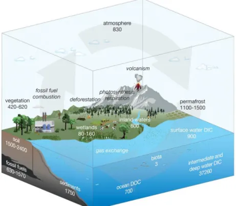
The effects of climate change are predicted to have a tremendous impact on human societies, some estimates reach economic damages of up to 20 % of GDP (Stern, 2006), with associated changes in water security (Haddeland et al., 2014), agriculture (Adams et al., 1998), and fisheries (Brander, 2010) leading to food and water shortages on local and regional scales (Haddeland et al., 2014; Wheeler and von Braun, 2013). These changes are likely to cause sociopolitical alterations (da Silva, 2004) and consequently severe adaptations of societies on local (Hunt and Watkiss, 2011) and global scales (Burrows and Kinney, 2016; Reuveny, 2007). These climatic changes are strongly influenced by atmospheric greenhouse gas concentrations and thus are coupled to the release and storage of carbon (Change, 2007; Figure 1, Mollenhauer et al., 2019). Sedimentation and burial of organic matter (OM) in marine sediments present an efficient natural way of removing carbon from the atmosphere (Bauer et al., 2013). The degradation of OM in benthic marine environments also plays an essential role as it determines the quantity of carbon ultimately sequestered in deep sediments (Arndt et al., 2013). The input of OM from different sources and its respective molecular composition is of particular interest, as the chemical characteristics of the OM constituents, the so-called “quality of OM”, govern the degree of biochemical processing in benthic microbial communities (Schmidt et al., 2014). However,

Figure 1: Major global reservoir sizes (bold) in Pg carbon and associated exchange flux mechanisms (italics). From Mollenhauer et al. (2019).

(7)

Manuel J. Ruben Page 6 of 77 the composition and quantity of OM buried in sediments changes substantially over space and time (Arndt et al., 2013).

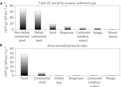
The immense size of the marine realm limits investigation into interactions of different sedimentary processes. Fjords, however, can be regarded as miniature oceans, offering a unique possibility to study processes in a defined space with accelerated rates (Skei, 1983). Despite the early recognition of the potential of fjord based studies, their role in marine carbon burial has only recently been highlighted by Smith et al. (2015) based on an extensive database study. These authors estimated that as much as 18 Mt of carbon are buried in fjords annually, which is equivalent to 11% of total annual carbon buried in marine sediments (Figure 2; Smith et al., 2015). Thus, normalized to their area fjords have by far the highest OM burial rates of any marine environment and can, therefore, be considered as “hot-sports”

for OM burial (Smith et al., 2015). A major reason for this is that in comparison to low-land costal systems, OM mobilized from terrestrial and petrogenic sources in fjords, has very low residence times in the mobilized state, leading to quick deposition and low mineralization during transport. OM residence time in fjords is generally highly influenced by climatic parameters like precipitation and temperature as well as local topography (Cui et al., 2017).

Even though Smith et al. (2015) entailed a wide variety of studies on OM burial in fjords (Cui et al., 2016c, 2017), only a few focused on arctic fjords (Cui et al., 2016a; Koziorowska et al., 2016). Nevertheless, Arctic fjords are of particular interest due to their high sedimentation rates, the associated poor sorting, and thus high rates of conservation and burial of OM (Bianchi et al., 2018). Furthermore,

arctic ecosystems are estimated to be most affected by climate change, a phenomenon known as

“Arctic Amplification” (Change, 2007), which results in increased heat uptake in the polar regions, due to shrinking snow and ice surface areas and a subsequent increase in polar albedo. This positive feedback will, cause strong alterations in the near future at high northern latitudes (Change, 2007).

Figure 2: Carbon burial of different oceanic sediment types in total (a) and area-normalized (b). From Smith et al. (2015)

(8)

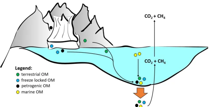
Manuel J. Ruben Page 7 of 77 Due to their sensitivity to climate changes, arctic fjords are an important focus for OM studies and have been underrepresented in past research (Bianchi et al., 2018). Arctic fjords can show high values of both biogenic and petrogenic OM leading to a complex mixture (Figure 3) of the total organic carbon (TOC) in the accumulated sediments (Walinsky et al., 2009). For the majority of arctic fjords, soils underlain by permafrost (Tarnocai et al., 2009) and/or glaciers are the primary sources of terrigenous organic matter accumulating in fjord sediments (Cottier et al., 2010). In today’s state of transitioning climate, both permafrost soils and glaciers have been found to be sources of pre-aged but labile OM being released from previously (freeze-) locked states into downstream aquatic systems, ultimately leading to an additional flux of carbon to the atmosphere, causing a positive feedback of climate warming (Hood et al., 2015, 2009; Winterfeld et al., 2018). Petrogenic organic matter represents ~90

% of organic carbon on earth, is the largest reservoir, and is primarily stored in shales and sedimentary rocks (Galy et al., 2008). Erosion related input due to transition from cold- to warm-based glaciers and runoff increase was estimated to release about 78 Tg of ancient particulate organic carbon and ancient dissolved organic carbon from glaciers into their adjacent aquatic systems by 2050 (Hood et al., 2015).

However, Hood et al. (2015) also stated that the reactivity of this ancient material has not been quantified and it is unclear to what extent the ancient OM can be re-mineralized in the downstream environments. Nevertheless, their incubation experiments suggested potentially high bioavailability of the investigated ancient material.

Figure 3: Scheme of possible organic matter sources, their transport and sedimentation to the ocean/fjord floor and subsequently into the sediment (brown arrow). Release of the greenhouse gases CO2 and CH4 into the water column and atmosphere,due to remineralization of organic matter in the marine sediments.

(9)

Manuel J. Ruben Page 8 of 77 Bio-availability and hence the potential for remineralization of this ancient OM is still highly debated.

The current understanding of OM utilization and thus remineralization expects “young”, “fresh”, and therefore “labile” OM to be preferentially utilized by organisms (higher energy yields) rather than

“old”, “ancient”, and therefore “recalcitrant” OM. This leads to the widely accepted concept of preservation and sequestration of ancient OM as opposed to reworking and remineralization processes (Guillemette et al., 2017). In contrast to this concept, recent research shows increasing evidence of utilization of ancient OM in settings where fluxes of ancient carbon are increased by both anthropogenic and natural sources (Cui et al., 2016a; Guillemette et al., 2017; Hood et al., 2015; Petsch et al., 2001; Wakeham et al., 2006). In arctic fjord systems, ancient POM often originates from the release of petrogenic sources excavated by glaciers (Cui et al., 2016a) and is subsequently being categorized as remnant and non-bioavailable. Anthropogenic aerosol particles derived from fossil fuel burning have been reported as another source of ancient carbon in glaciers, supplying the majority of fossil DOM to glacial environments (Stubbins et al., 2012). In turn, “young” and labile OM is also produced within the fjord’s water column, local soils (Cui et al., 2017) and glaciers (Hood et al., 2015).

Hence, a complex assemblage of OM from diverse sources and ages comes into play (Figure 2), which may change the overall dynamics of the refractory fraction (Guillemette et al., 2017). The input of fresh and labile material has been noticed to enhance the bio-availability and lability of OM over all in soils.

This complex and not yet fully understood process of “priming” (Bianchi, 2011; Fontaine et al., 2003;

Guillemette et al., 2017) has also been described to enhance refractory OM degradation in marine sediments, especially at high OM concentrations in sediments (Gontikaki et al., 2013). Hence, it may be essential for remineralization of ancient OM in arctic fjord sediments studied in this thesis (Guillemette et al., 2017), but also in a wider picture as 40 % to 50% of the organic carbon buried in arctic sediments derive from supposedly recalcitrant petrogenic OM (Drenzek et al., 2007). With remineralization and preservation of OM playing a key role in regulating atmospheric greenhouse gas levels in the long run (Bauer et al., 2013), the estimation of the changing OM composition and resulting remineralization of the distributed OM is essential for future predictions and models (Arndt et al., 2013; Guillemette et al., 2017).

(10)

Manuel J. Ruben Page 9 of 77 Organism specific biomolecules, so-called biomarkers can be used to assess different sources of organic matter in an ecosystem.

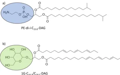
For this purpose, solvent extractable lipid biomarkers offer great potential in sedimentary studies. Different compound classes like n-alkanes, n-alkanoic acids (fatty acids; FA), glycerol dialkyl glycerol tetraethers (GDGTs), and homohopanoids (Figure 5) in combination with their respective number of carbon atoms, isomeric structure, and isotopic signature are indicative for different precursor organisms, environmental, or depositional conditions. These biomarkers are classically used due to their high resilience to degradation (Bianchi and Canuel, 2011). In contrast, IPLs (Figure 4) are widely seen as indicators of living biomass, as these lipids are prone to a quick loss of their head groups within days to weeks after cell death through natural breakdown mechanisms. This class includes glycol-, phosphor-,

and amino-lipids, which in turn are diagnostic for precursor organisms in combination with their respective side chains (Sturt et al., 2004). These compound classes can be separated by wet chemical preparation to obtain fractions of compounds indicative of viable and non-viable microbiota (Akondi et al., 2017; Ringelberg et al., 1997;

Wakeham et al., 2006).

In order to trace different OM-pool inputs to marine sediments on a decadal to millennial time scale, a combined approach of biomarker analysis with bulk and compound CSRD has been proven to be an effective tool to identify (residence) ages of OM accumulated in sediments (Feng et al., 2013;

Mollenhauer and Rethemeyer, 2009; Vonk et al., 2017, 2012; Winterfeld et al., 2018). Additionally,

Figure 5: Examples for (remnant) biomarker classes used in this study

Figure 4: Phospho-(a) and glycolipid (b) examples for labile intact polar lipids and associated fatty acid side chains. Ovals indicate head groups lost quickly after cell lysis from core lipids.

(11)

Manuel J. Ruben Page 10 of 77 CSRD of IPLs can be used to identify metabolic pathways of modern versus ancient organic compounds in sediments, using ¹⁴C as an inverse-tracer. ¹⁴C is an ideal tracer signal as it can be carried over from the substrate to the utilizing microorganisms, allowing for the biological assimilation of degrading microbiota to be identified through their respective radiocarbon age (Petsch et al., 2001; Slater et al., 2006a; White et al., 2005). In turn, this approach determines if and to what extent, local benthic microbial communities are able to utilize ancient OM. If the ancient OM would entirely consist of non- bioavailable and therefore remnant biomass, extracted FA of IPLs would show modern ¹⁴C activity levels as they would exclusively metabolize recently assimilated biomass, in accordance to the principle

“you are what you eat”. On the contrary, ¹⁴C signatures below the modern endmember indicate the possibility of the microbial community to utilize ancient OM as a carbon or energy source for their metabolism. The latter case would suggest ancient carbon utilization by microbes, which would have to be accounted for in future climate models and predictions.

1.1 Goals and Hypotheses

This study investigates changes in sedimentary OM composition, their rates of deposition, and remineralization in Hornsund Fjord, Svalbard, over the course of the last 60 years using lipid biomarkers, bulk OM parameters and CSRD. It addresses the hypothesis that changing environmental conditions influence OM production and mobilization. The strong warming of recent decades is expected to result in an overall increase in carbon exported from glaciers and adjacent soils to local fjord sediments.

More specifically, the working hypothesis (1) suggests that increasing atmospheric temperatures lead to higher glacial runoff and higher amounts of petrogenic carbon being exported to downstream aquatic environments. However, with shifting glacial fronts petrogenic OM input may decrease at a given core location over time. Simultaneously, increased runoff leads to higher turbidity in downstream aquatic systems, causing a decrease in marine primary production, due to less sunlight penetration into the photic zone. However, with retreating glaciers this effect may lose its significance as the inflow of turbid waters will follow the glacial front while the ice-free sea surface area will simultaneously increase, in turn leading to a larger area of sunlight penetrating into the sea surface layer. Furthermore, increasing temperatures and decreasing salinity may exert a strong influence on local aquatic primary productivity. Both parameters have to be considered as they are directly or indirectly influenced by atmospheric temperatures and glacial runoff.

(12)

Manuel J. Ruben Page 11 of 77 Secondly, the uptake of ancient carbon by benthic microbial communities is investigated. It is hypothesized that the mobilization of ancient terrigenous organic matter to arctic fjords will contribute to greenhouse gas emissions due to the microbial degradation of ancient carbon in the marine realm.

Specific working hypothesis (2) is that due to the long ongoing, continuous input of ancient OM, local microbial communities have adapted to utilize ancient OM for anabolic and catabolic purposes. Taking into account the principle of “you are what you eat” of the isotopic signature, ancient OM utilizing microbiota are expected to show ¹⁴C-depleted radiocarbon signatures. Nevertheless, if – despite short residence times – remineralization of ancient OM is occurring in the water column already, these microbiota may be exported to the sediment where they could further utilize ancient OM when buried.

Downcore profiles will show different stages of OM utilization from freshly deposited sediment (core top) to more mature stages (down core). Allowing a temporal view of the remineralization dynamics.

Information about sedimentary OM input (derived from working hypothesis 1) will allow in-depth analysis of the utilized substrate by heterotrophic microbiota using a ¹⁴C endmember model.

Additionally, it is hypothesized (3) that OM degradation by benthic microbial communities is initiated/primed by supply of highly bioavailable organic matter, i.e., from phytoplankton, and will extend to less bioavailable petrogenic organic matter, due to the continuing presence of previously released exoenzymes or other metabolites. This is expected to result in a temporal shift in the radiocarbon signature of the biomarkers (fatty acids) originating from degrading microorganisms. In early stages of degradation (core top), the indicative biomarkers are expected to have a relatively young signature. With increasing time/depth these radiocarbon signatures are expected to shift to older values. However, the possibility of changes in the primary input of modern and ancient OM has to be taken into consideration while assessing this hypothesis, as this is expected to have a strong impact on the radiocarbon signature of the indicative biomarkers. Ideally, two (or more) samples taken from the same sediment depth, at the same location, but retrieved considerable time apart from one another, would be needed to assess this hypothesis. Nevertheless, by assessing both the OM input to the sediment and the compound specific radiocarbon signatures, a reliable estimation of the importance of priming for the utilization of ancient carbon in arctic fjord sediments will be determined.

(13)

2. Methodology

2.1 Study Area and sampling

The Svalbard archipelago is located between the Arctic Ocean in the north, the North Atlantic in the south and the Barents Sea to the east. On Svalbard’s western flank, the Fram Strait is strongly influenced by the West Spitsbergen Current bringing warm and saline Atlantic water to the north, being the primary salt and heat source to the Arctic ocean (Mangerud et al., 2006; Muckenhuber et al., 2016).

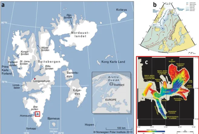
This results in the relatively mild climate on Svalbard and an overall low ice cover of the eastern Fram Strait (Onarheim et al., 2014). Hornsund Fjord is located at the far south-west of Svalbard (Figure 6).

Its location causes a strong influence by cold and low saline Arctic-type waters of the Sørkapp (Costal) Current originating in the Barents Sea, which separates the local microclimate from the other fjords on Svalbard’s western coast (Koziorowska et al., 2018). This is of particular importance as local conditions are dominant factors for seasonal sea ice formation rather than large-scale atmospheric and oceanic conditions (Muckenhuber et al., 2016), and therefore are highly susceptible to climatological and hydrological fluctuations (Majewski et al., 2009). Seasonal ice cover is important factor for glacial runoff (Kohler et al., 2007), water column stratification and overturning (Cottier et al., 2010), primary production (Smoła et al., 2017), benthic meiofaunal assemblage (Grzelak and Kotwicki, 2012), and burial and sequestration of carbon (Koziorowska et al., 2018). South-West Svalbard’s location right on the outer edge of the arctic front makes it highly influenced by global climate change, especially due to Arctic Amplification (Change, 2007), which will in turn also influence local climatic conditions. Thus, current regional processes may be indicative for future regional changes.

Hornsund Fjord comprises of a main basin, connecting multiple smaller side bays to a system of about

~ 32 km length and ~ 10 km width. The glaciers’ proximal basins are separated by sills in depths of ~ 100 m from the main fjord basin which is > 250 m deep (Pawłowska et al., 2017). Its complex catchment spans over about 1200 km² with 73 % glaciated area (Szczuciński et al., 2006) of which 97 % constitutes thirteen tidewater glaciers. Five of the most active glaciers are located in the innermost basin, Brepollen. With changing climatic conditions these local tidewater glaciers retreated with rates of several tens to 120 m yr^-1 (Błaszczyk et al., 2013), creating expanding bays (Ziaja, 2001) while simultaneously forming “sediment traps” in the inner bays like Brepollen. In these bays, fast ice formation during winter is common, whereas in the central basin sea ice formation varies from one year to the next (Błaszczyk et al., 2013). Local tidewater glaciers supply vast amounts of sediment, reaching sediment accumulation rates of up to 0.7 cm yr^-1 (Szczuciński et al., 2006). During summer,

(14)

Manuel J. Ruben Page 13 of 77 meltwater runoff increases drastically leading to strong stratification at Brepollen bay. Associated high loads of suspended inorganic material limits the euphotic zone and consequently primary production (Grzelak and Kotwicki, 2012). However, local primary production rates are still relatively high with rates up to 120 to 220 g C m^-2 yr^-1(Piwosz et al., 2009; Smoła et al., 2017). Leading to high sedimentary organic carbon concentrations ranging from 1.38 % to 1.98 % (Koziorowska et al., 2016). Most contributing primary producers are diatoms, with increasing dominance towards the fjord mouth, and nanoflagellates (Piwosz et al., 2009). Due to extensive glaciation, the exposed terrestrial terrain in the catchment area of Brepollen is extremely small and its time of exposure is limited to the recent decades of fast glacial retreat (Błaszczyk et al., 2013). Hence, biomarker concentrations of recently produced terrestrial OM and soils are expected to be negligible for the investigated sediment core and sedimentary OM input can be assessed by using two-endmember models of marine and petrogenic biomarkers.

The location of Hornsund Fjord at the arctic frontal region and the associated strong climatic changes (Saloranta and Svendsen, 2001) make it a key study area to investigate changes in OM cycling as part of the global carbon cycle. For this study, sediment samples were taken from gravity core HH14-897-

Figure 6: a) Map of Svalbards’ fjords, glaciers (indicated in white), and non-glaciated areas. b) North Atlantic currents indicating Svalbards location on the Arctic front (Mangerud et al., 2006). c) Bathymetric map of the Brepollen bay, location in a) indicated by red rectangle (personal correspondence Forwick, 2019) and marking coring location of HH14- 897-MF-GC (magenta star).

(15)

Manuel J. Ruben Page 14 of 77 GC-MF. It was obtained on board of the RV Helmer Hanssen in October 2014 in the most proximal bay of Hornsund Fjord, Brepollen, in a water depth of 140 m (Figure 1).

2.2 Age model

The age model was created by Szczuciński (2019, personal communication, AMU) on the basis of a ²¹⁰Pbxs constant initial concentration (CIC) model after Robbins and Edgington (1975), verified with ¹³⁷Cs peaks for 1963 and 1986. Measurements were performed every 2 cm downcore, allowing the construction of a high- resolution age model. The ²¹⁰Pbxs and ¹³⁷Cs data were obtained at the Department of Mineralogy and Petrology at Adam Mickiewicz University, Poland using gamma spectrometry. The age model was cross-checked by comparison to reconstructed glacial forefronts (Błaszczyk et al., 2013), coring date, laminations visible in X-ray scans, and sediment thickness.

2.3 Sampling and sample preparation

Organic compounds for biomarker analysis were extracted from 22 sediment samples throughout the core. Sampling depths were chosen on the basis of the age model provided by Szczuciński (2019, personal communication, AMU). The age model indicates the earliest sample age for the biomarker analysis at 1961 AD and the youngest at the core top at 2014 AD, leading to a biogeochemical archive of 53 years (Table 1).

Further, five large volume samples were taken for CSRD (Table 2). In order to obtain lipids in sufficient quantities to allow compound specific radiocarbon dating (CSRD) the sample size chosen was larger than for the classic biomarker abundances samples. In total 5 samples were taken of the archive half of gravity core HH14-897-GC-MF. Each sample was taken over a depth interval of 3 cm. To obtain as much sample volume as possible the whole core section was used. However, the outer edges of the sediment-cake were removed to prevent contamination from the liner and from carry-over. All samples were stored in pre-combusted glass containers at -20°C, freeze-dried, and then homogenized in an agate mortar.

Depth [cm]

Year of Deposition,

A.D.

Dry weight

[g]

1.5 2011 3.01

4.5 2005 3.01

8 2000 3.05

13 1993 3.00

16.5 1990 2.99

19 1989 3.01

22 1987 3.03

25 1986 3.10

28 1986 3.01

31 1985 3.04

34 1983 3.02

43.5 1982 3.03

53.5 1980 3.07

60 1978 3.09

73.5 1975 3.00

83.5 1973 3.07

96 1971 2.99

103 1969 3.01

113 1967 3.01

123 1965 3.07

133 1962 3.09

137.5 1961 3.03

Table 1: Depth, age, and weight of the samples used for biomarker abundances. Ages: dated by Szczuciński (green) and interpolated (blue)

Depth interval

[cm]

Year(s) of Deposition,

A.D.

Dry weight

[g]

0-3 2014-2008 60.67 5-8 2004-2000 77.20 10-13 1997-1993 76.56

86-89 1972 81.83

133-136 1962 82.29

Table 2: CSRD samples, time of sedimentation and dry weight of sediment extracted off.

(16)

2.4 Sample processing

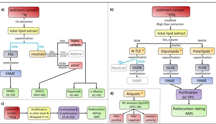
The general workflow of laboratory procedures used for this thesis is shown in Figure 7. Different procedural steps are displayed and linked to their respective analytical methods (green boxes). As displayed, the working methods were split into four procedures. In the following chapter, the individual methods are described. All used glass-ware were pre-combusted overnight at 450°C.

2.5 Bulk OM radiocarbon dating

Sample sizes were determined by the sample’s respective TOC content. Sediment samples for this thesis were consistently ~2 wt% TOC. In order to get target carbon concentrations of 1 mg C for accelerator mass spectroscopy (AMS), 50 - 60 mg of sediment were separated in small silver boats (Figure 7c). For each sample, two aliquots were weighed successively into silver boats, the second one being considerably smaller (~10 %) as it would later function as a pre-sample to clean the system. The sediment in the silver boats was acidified with super-pure 6 M HCl to remove inorganic carbon and subsequently dried on a hotplate at 60°C, three consecutive times. After the third acidification samples were dried overnight at 60°C. Subsequently, silver boats were folded tightly and wrapped into tin foil.

Figure 7: General lab work workflow for a) biomarker abundances, b) CSRD, c) bulk radiocarbon, and d) IPL analysis (performed for all three fractions) – Box color codes are as followed, dark red: sediments; yellow: total lipid extracts; orange: unsaponified lipids; red *: link between workflow b) and d); dark blue: fatty acid fractions; bright blue: fatty acid methyl ester; bright red:

fractions of neutral lipids; purple: technical preperative procedures; green: analytical methods used; pink: QqTOP modes used for samples; grey: extracted and stored fractions, but not used in this study. Black lines, arrows and text modulars: used and discribed methods inluding solvents; Blue arrows: indicate liquid-liquid extraction inluding solvents; Dashed black arrows: no procedual advancment, but different analytical mode.

(17)

Manuel J. Ruben Page 16 of 77 At first, one pre-sample was run to clean the system from any contaminants, the actual sample was run thereafter. Prepared samples were combusted in an Element Analyzer (EA) at 950°C in a constant flow of helium with the addition of oxygen. Emitted combustion gases were completely oxidized by excess oxygen and copper oxide in the combustion tube. The sample packages were made of tin foil which functioned as a catalyst. The resulting gas-mixture was composed of CO2, N2, and H2O.

Subsequently, the three gases were separated by chromatography. The purified CO2 gas was transferred to an Automated Graphitization Equipment (AGE), where the transferred CO2 gas from EA combustion was absorbed and concentrated on a zeolite trap and the other gases were vented. After the complete transfer, the zeolite trap was heated to a temperature of 450 °C. Due to thermal desorption and associated thermal expansion of the trapped CO2 gas, it was released and transferred into a pre-evacuated quartz glass vial attached to the reactor chamber, and heated up to 580°C after gas injection. A local hydrogen atmosphere in the presence of an iron catalyst completely reduced the inflowing CO2 gas from the zeolite trap within the vial, and caused graphite to precipitate on the surface of the iron powder the vial. The resulting graphite was pressed into targets and later measured using AMS. Recovered graphite pellets were further pressed into targets before determining their respective F¹⁴C using AMS at the MICADAS lab in Bremerhaven (AWI, compare section 2.7.7).

2.6 Biomarker Analyses

2.6.1 Lipid extraction

Lipid biomarkers were extracted in a multistep (Figure 7a) procedure from ~ 3 g of the dry, ground and homogenous sediment by

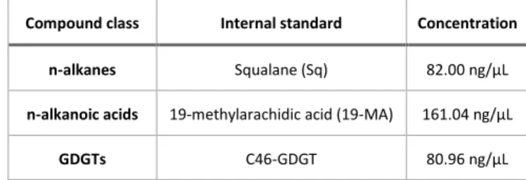
ultrasonic extraction (3 x 15 min, at room temperature) with three times 25 mL of a mixture of dichloromethane (DCM) and methanol (MeOH) in a volumetric ratio of 9:1. For quantification of the different lipid classes, 10 µL of an internal standard mixture (Table 3) was added to the weighed sediment (Table 1) prior to extraction.

2.6.2 Saponification and separation of fatty acids

After extraction, the total lipid extracts (TLE) were saponified in 1.5 mL (CSRD: 15 mL) of a solution of 0.5 M KOH in MeOH:H2O 9:1 (v:v) for 2 hours at 80°C, cleaving off FAs from their respective precursor molecules forming more polar, dissolved FA potassium salts. From this mixture, the remaining neutral lipids were separated three times using 1.0 mL (CSRD: 10 mL) n-hexane (HEX) in liquid-liquid phase separation. Subsequently, the residual solution of the TLE containing the organic salts was re-acidified

Compound class Internal standard Concentration

n-alkanes Squalane (Sq) 82.00 ng/µL

n-alkanoic acids 19-methylarachidic acid (19-MA) 161.04 ng/µL

GDGTs C46-GDGT 80.96 ng/µL

Table 3: Internal standards used for biomarker quantification

(18)

Manuel J. Ruben Page 17 of 77 to FAs using hydrochloric acid until reaching a pH-value of 1. FAs were further purified by three times liquid-liquid phase separation using 1.0 mL (CSRD: 10 mL) DCM. This procedure resulted in one fraction each for neutral lipids and FAs.

2.6.3 Silica gel column chromatography

In the following sections, different wet chemical procedures are described.

Within these protocols liquid chromatography is used for compound separation and purification. Different compound classes were eluted from the stationary phase (column) by selected mobile phases (solvents), due to their individual polarities and the compounds’ respective interactions between stationary and mobile phase(s). Although the mobile phase changed due to different procedural requirements, the stationary phase was consistent.

As stationary phase, a silica column was set up for each individual separation (Figure 8: Silica column setupFigure 8). For this purpose, 1 g of pre-combusted

silica gel (SiO2, deactivated with 1 % H2O) suspended in HEX was loaded into a 4 mL pre-combusted glass pipette, resulting in a silica column length of 4 cm. In order to prevent silica gel from discharging off the pipette and entering the purified fractions, the bottom of the pipette was filled with pre- combusted glass wool prior to loading. Additionally, an ~5 mm thick layer of Na2SO4 was added on top of the silica gel to prevent any H2O from entering the column and interfering with its polarity properties. Subsequently, compounds were loaded onto the column by three times 100 µL of the eluting solvents described in 2.6.4,2.6.5, and 2.7.3 before the mobile phase was added.

2.6.4 Methylation and purification of fatty acids

FA fractions were methylated overnight in a MeOH:HCl37% 95:5 (v:v) solution at 50°C, forming less polar fatty acid methyl ester (FAME). The isotopic signature of the used MeOH was determined prior to methylation. Obtained FAMEs were further purified by column chromatography to remove remaining polar components. Silica gel was used as a stationary phase (compare section 2.6.3) with two different mobile phases. First FAMEs were eluted using 4 mL DCM:HEX 2:1 (v:v) followed by the second phase, eluting polar compounds with 4 mL DCM:MeOH 1:1 (v:v). The purified FAMEs were quantified by gas chromatography (GC) – flame ionization detector (FID).

Figure 8: Silica column setup. Glass pipette, filled with glass-wool (dark gray), silica gel (light gray), and Na2SO4

(white).

(19)

Manuel J. Ruben Page 18 of 77 2.6.5 Neutral lipid separation

Neutral lipids were separated into three fractions over a pre-combusted silica column (compare section 2.6.3). Fraction one was eluted first with 4 mL HEX, containing non-polar components, primarily n-alkanes. Secondly, ketones were eluted with 4 ml of DCM:HEX 2:1 (v:v) into fraction two. At last, fraction three was eluted with 4 ml of DCM:MeOH 1:1 (v:v), containing the most polar compounds of the neutral lipids like alcohols and GDGTs. After separation n-alkanes and ketones were quantified by GC-FID. Whereas, polar components of alcohols and GDGTs were dissolved in HEX:2-propanol 99:1 (v:v) and filtered through a 0.45 μm syringe filter to remove any particles before quantification by high performance liquid chromatography (HPLC) – mass spectroscopy (MS), homohopanes were quantified in the n-alkane fraction using GC-MS and an external hopane standard.

2.6.6 Gas Chromatography – Flame ionization detector

Extracted n-alkanoic acids (measured as FAME) and n-alkanes were identified and quantified on a GC- FID, using internal, external, and reference standards and their respective retention times. A 7890A gas chromatograph (Agilent Technologies) equipped with a DB-5MS fused silica capillary column (60 m, ID 250 µm, 0.25 µm film coupled to a 5 m, ID 530 µm deactivated fused silica precolumn) and a FID was used (Figure 9).

Extracted samples were dissolved in 100 µL HEX for injection with the cold on-column injection system.

Injection volume was 1µL of the sample solution. The GC was heated using the following temperature program: 60 °C for 1 min., 20 °C/min. to 150 °C, 6 °C/min. to 320 °C and a final hold time of 35min.

Compounds were carried by a constant flow of helium of 1.5 µL min^-1. In the FID the compounds were combusted with a fuel gas mixture of hydrogen and synthetic air.

In order to minimize contamination, the system was cleaned with two runs of HEX before each sample batch. Additionally, the syringe of the injection system was automatically cleaned with DCM and HEX before and after each injection.

(20)

Manuel J. Ruben Page 19 of 77 2.6.7 Gas Chromatography – Mass spectrometry

For identifying compounds in very low concentrations, i.e. hopanes, or without a specific reference standard, a GC-MS system was used. The setup consisted of an Agilent 6850 GC coupled to an Agilent 5975C MSD operating in electron impact mode with an ionization energy of 70 eV. The GC was equipped with a fused silica capillary column (Restek Rxi-1ms, length 30 m; 250 µm ID, film thickness 0.25 µm). Compounds dissolved in HEX were injected in split-less mode in the injector held at 280 °C, with an injection volume of 1 µL. Helium was used as the carrier gas at a constant flow rate of 1.2 mL/min. The GC temperature program was as follows: 60 °C start temperature, held for 3 min, increased to 150 °C with a rate of 20 °C min⁻¹, increased further to 320 °C with a rate of 4 °C min⁻¹and finally held at 320 °C for 15 min. The source temperature of the MS was set to 230 °C and the quadrupole to 150 °C. After GC separation, compounds were fragmented into ions, accelerated, deflected and finally their mass to charge ratio (m/z) was determined in full-scan mode.

In order to minimize contamination, before every batch, a cleansing run with pure HEX was performed.

In addition, the syringe for sample injection was automatically cleaned with DCM and hexane before and after each injection.

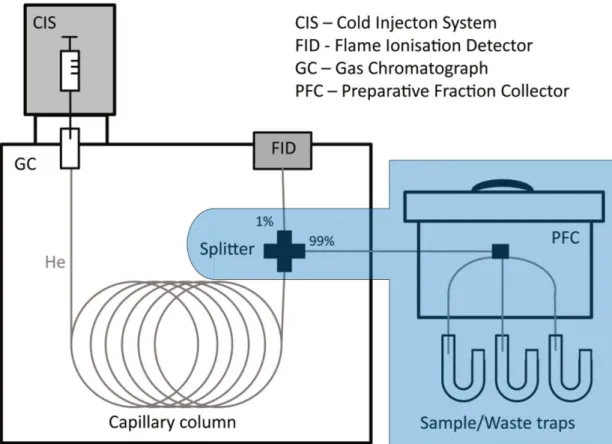
Figure 9: Building blocks of GC-FID (without blue box) and GC-PFC (with blue box) modified after Höfle (2015)

(21)

Manuel J. Ruben Page 20 of 77 2.6.8 High-performance liquid chromatography – Mass spectrometry of GDGTs

GDGT were analyzed after a slightly modified protocol from Hopmans et al. (2016), using an Agilent 1200 series HPLC system with two consecutively linked UPLC silica columns in series (Waters Acquity BEH HILIC, 2.1 x 150 mm, 1.7 µm) and a 2.1 x 5 mm pre-column of the same material, maintained at 30 °C. The HPLC setup was connected to an Agilent 6120 MSD, allowing an atmospheric pressure chemical ionization (APCI) interface linkage to a single quadrupole MS. Two mobile phases were used, mobile phase A (HEX/2-propanol; 99:1, v/v) was used 5 minutes into each sample run and for 15 min prior to the next sample to re-qeuilibate with 18 % of mobile phase B (HEX/2-propanol/chloroform;

89:10:1, v/v/v). After sample injection (20 µL) and 25 min isocratic elution with 18 % mobile phase B the proportion of B was linearly increased to 50 % within 25 min, and thereafter to 100 % for the next 30 min. Flow rate was 0.22 ml/min and a maximum back pressure of 220 bar was obtained. Total run time was 100 min.

At the APCI-MS a positive-ion mode was used with a selective ion monitoring for their (M+H)+ ions or ion-source fragmentation products to identify GDGTs (Schouten et al., 2007) and OH-GDGTs (Liu et al., 2012). APCI spray-chamber conditions were as follows: nebulizer pressure 50 psi, vaporizer temperature 350 °C, N2 drying gas flow 5 l/min and 350 °C, capillary voltage (ion transfer tube) -4 kV and corona current +5 µA.

GDGT concentrations were determined using the response factor form a C46 GDGT standard, by integrating respective peak areas. Due to a lack of appropriate standards, individual relative response factors between the different GDGTs and the C46 were not determined. The obtained concentrations should therefore be regarded as being only semi-quantitative.

2.7 Compound specific radiocarbon dating of fatty acids

2.7.1 Pre-extraction sample preparation

FAs were extracted, separated, and purified using a sequence of wet chemical techniques and chromatographic methods (Figure 7b).

2.7.2 Lipid extraction

Organic compounds were extracted and separated using a modified Bligh and Dyer approach in combination with liquid chromatography over a silica column (Akondi et al., 2017; Bligh and Dyer, 1959; Slater et al., 2006b; Wakeham et al., 2006).

(22)

Manuel J. Ruben Page 21 of 77 To maximize lipid yields, the entire sediment samples (Table 2) were used for extraction. Extraction was carried out overnight (~18 hours), at room temperature with a single-phase solution of DCM:MeOH:PO4B in a volumetric ratio of 1:2:0.8. The phosphate buffer (PO4B) was prepared by dissolving 4.35 g of dibasic potassium phosphate in 500 mL of nano-pure water. The buffer was then set to a pH-value of ~7.4 using HCl. After the initial extraction, the remaining sediment was rinsed twice with 100 mL of the extraction solution and ultrasonicated. The resulting solvent lipid extract was filtered and collected in a separatory funnel. DCM and purified H2O were added to the separatory funnel until a ratio of DCM:MeOH:[PO4B+H2O] in 1:1:0.9 (v:v:v) was reached. Additionally, KCl was added to enhance the separation process of the resulting two-phase system. Subsequently, the solvent lipid extract contained in the DCM phase was drained, and the aqueous phase was re-extracted twice with DCM, before the combined DCM extracts were evaporated by a rotary evaporator.

2.7.3 IPL separation through liquid chromatography Depending on their visual appearance the TLEs were separated into 2 to 5 aliquots, to minimize the risk of column overloading in the following separation procedure. The separation of the lipids into three different fractions was achieved according to their

polarity reflected in their interaction with the silica column during column chromatography (Table 4).

For the column, the setup is described in the section 2.6.3. Compounds were eluted with three different solvents starting from low to high polarity. First, non-polar compounds and triacyclglycerols (TAG) were eluted with 4 ml DCM, followed by free FA and glycolipids (GL) with 4 ml Acetone and by polar lipids (PL) such as phospho- and amino lipids with 4 ml MeOH. To simplify the following working process the aliquots of the different polarity fractions were re-combined.

2.7.4 Derivatization of fatty acids

Ester bonds between core-lipids and the FA side-chains were broken by mild alkaline saponification with 0.5 M KOH in MeOH:H2O 9:1 (v:v) for 2 hours at 80°C (compare: section 2.6.2), in all three fractions. Neutral lipids of the non-polar fraction were extracted after saponification with HEX, this fraction was dried and stored. The residual of the non-polar-, GL-, and PL-fraction were re-acidified and FA were extracted with DCM. Subsequently, the FAs were methylated into FAMEs and cleaned via silica column. The procedures used were equivalent to the ones used for determination of biomarker abundances.

Solvent Fraction

DCM neutral lipids (NL) Acetone glycolipids (GL) MeOH polar lipids (PL)

Table 4: During IPL separation used solvents and related fractions.

(23)

Manuel J. Ruben Page 22 of 77 2.7.5 Gas Chromatography – Preparative fraction collector

Purified FAME fractions extracted from large samples for CSRD contained a multitude of different compounds varying in chain lengths, degrees of unsaturation, and isomers. In order to obtain pure single compound FA fractions, samples were purified using a gas chromatograph coupled to a preparative fraction collector (GC-PFC; Eglinton et al., 1996).

The schematic setup is shown in Figure 9. A traditional GC-FID unit is coupled with an additional PFC.

GC, and FID working principles and temperature program were as described in section 2.6.6. In the GC- PFC setup, a Gerstel Cooled Injection System (CIS) connected to an Agilent HP6890N GC equipped with a Restek Rtx-XLB fused silica capillary column (30 m, 0.53 mm diameter, 1.5 μm film thickness) was used. In this setup, a splitter separates the gas flow from the capillary column, causing a distribution of the flow to 1 % to the FID and 99 % to a Gerstel PFC. The FID unit determines retention times of target compounds. The PFC was equipped with six pre-combusted glass sample traps and one waste trap. Every outlet of a trap is connected to an individual magnetic valve, of which only one can be opened at a given time. All traps were kept at room temperature, allowing the compounds to condense in the traps while entering. The PFC top unit was constantly kept at 340 °C (maximum temperature reached at the GC) to prevent any compound precipitation before the eluent entered the glass traps.

Purified compounds were later transferred with DCM from the glass traps to pre-combusted glass vials.

For purification, the fatty acid fractions were dissolved in HEX. Depending on the concentration in the solution, it was injected up to 100 times (100 GC runs) with 5µL each time. The degree of dilution was chosen according to target compound concentrations, aiming for maximum compound concentrations while staying below 5 µg for a single compound to prevent column overloading and coelution. The purity of the isolated single compounds was evaluated by GC-FID and GC-MS.

In order to minimize contamination, the syringe of the CIS was automatically cleaned with DCM and hexane before and after each injection. In addition, before every new sample the deactivated glass liner in the CIS was exchanged and a cleansing run with pure hexane was performed.

2.7.6 Radiocarbon measurements

Purified compounds were measured as CO2 gas at the MICADAS-facility of the Alfred-Wegener- Institute in Bremerhaven, Germany. The purified compounds were washed into tin capsules for liquids (25 µl volume, 2.88x6x0.1 mm, Elementar) three times using DCM. Volumes were chosen appropriately to generate sample sizes between 10 and 100 µg C. After the solvent was completely evaporated, tin

(24)

Manuel J. Ruben Page 23 of 77 capsules were folded and combusted using a vario isotope select elemental analyzer. Resulting CO2

gas was directly injected into the MICADAS ion source under constant flow and pressure. Samples were corrected for both machine blank against ¹⁴C free CO2 gas using BATS software (Wacker et al., 2010) and procedural blanks (compare: below).

2.7.7 Accelerator mass spectrometry

Radiocarbon dating was performed on an accelerator mass spectrometer using the Mini Carbon Dating System (MICADAS 15; Wacker et al., 2010), produced by Iongplus AG. Both graphitized sediment (compare: section 2.5) samples as well as the purified FAME were measured on this system. The system uses an optimized cesium ion source, allowing sample sizes as small as 10 µg C. Graphitized bulk OM samples were loaded as pressed targets directly into the AMS. Whereas, prepared samples for CSRD were combusted in an EA (compare: section 2.5). Generated CO2 gas was trapped on a zeolite trap in the Gas Ion Source Interface. After completed combustion, the CO2 gas was released from the trap by heating the trap to 450°C. Emitting CO2 gas was quantified manometrically after desorption from the trap and subsequently diluted to 5 % in He. The resulting gas mixture was directly injected into the AMS ion source under constant flow and pressure.

In the AMS, both sample types were ionized by an accelerated ion beam (Cs⁺) causing negatively charged carbon ions to shutter of the samples, allowing a discrimination of ¹⁴C against ¹⁴N.

Subsequently, all ions are accelerated into the focusing device and deflected by an injector magnet to split off non-carbon-ions. Remaining carbon ions are accelerated in a tandem accelerator unit and bypass an electron stripper, scattering remaining molecules. Subsequent carbon atoms are further accelerated and deflected by their mass due to a second magnet to remove remaining molecule fragments. Emerging carbon ion beams are quantified by their amperage using a Faradey cup.

All radiocarbon data were normalized relative to the reference standard oxalic acid II (NIST 4990c) and expressed in fraction of modern carbon (F¹⁴C) for post-bomb samples to avoid confusion with different terms (Reimer et al., 2004):

𝐹¹⁴𝐶 = (¹⁴𝐶/¹²𝐶_{𝑠𝑎𝑚𝑝𝑙𝑒})

(¹⁴𝐶/¹²𝐶_{𝑠𝑡𝑎𝑛𝑑𝑎𝑟𝑑}) (1)

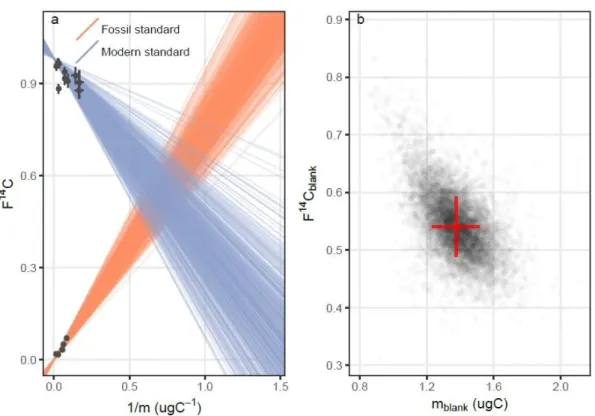
2.7.8 Blank correction

Due to the extremely small sample size and extensive wet chemical processing, the obtained ¹⁴C data is potentially influenced by carbon contamination and procedural blanks. In order to obtain correct

(25)

Manuel J. Ruben Page 24 of 77 radiocarbon data for the investigated samples, a blank correction was performed. The carbon contamination from sample processing is too low to be determined directly (< 10 µg C). Influence of the blank carbon on the mass and F¹⁴C of samples increases with decreasing sample size. Therefore, it is necessary to perform a secondary blank correction. Sample processing blanks (b), including wet chemical processing, sample combustion and measurement, were determined by processing standards (std) of known ¹⁴C composition. FAMEs extracted from Messel Shale (F¹⁴C = 0; immature Eocene oil Shale from western Germany) and Apple Peel (F¹⁴C = 1.031 ± 0.004) were processed similarly to the investigated samples. Assuming constant contamination it is possible to indirectly determine the processing blank by analyzing FAMEs of different masses (m) and known ¹⁴C composition, using a standard mass balance (Hwang and Druffel, 2005):

𝐹¹⁴𝐶𝑠𝑡𝑑+𝑏∗ 𝑚𝑠𝑡𝑑+𝑏 = 𝐹¹⁴𝐶𝑠𝑡𝑑∗ 𝑚𝑠𝑡𝑑+ 𝐹¹⁴𝐶𝑏∗ 𝑚𝑏

= 𝐹¹⁴𝐶_𝑏∗ 𝑚_𝑏+ 𝐹¹⁴𝐶_𝑏∗ (𝑚_{𝑠𝑡𝑑+ 𝑏}− 𝑚_𝑏) (2) Assuming a constant procedural blank equation (2) can be expressed as a linear equation, with 1/mstd + b representing the x-variable and F¹⁴Cstd + b the y-variable. The resulting y-intercept of the linear equation being the true F¹⁴Cstd value of the used standard and relating in (F¹⁴Cb-F¹⁴Cstd) as the slope of the linear regression (Hwang and Druffel, 2005):

𝐹¹⁴𝐶_{𝑠𝑡𝑑+ 𝑏}= (𝐹¹⁴𝐶_𝑏− 𝐹¹⁴𝐶_𝑠𝑡𝑑) ∗ 𝑚_𝑏∗ 1

𝑚_{𝑠𝑡𝑑+𝑏}+ 𝐹¹⁴𝐶_𝑠𝑡𝑑 (3) Therefore, linear regression lines for multiple fossil and modern standards were fitted to determine the blank (Hwang and Druffel, 2005). A Baysiean regression model was employed to account for measurement uncertainties and to calculate the intercepts (x0;y0) of the two regression lines, to determine 1/mb and F¹⁴Cb. The calculated carbon contamination accounted for a mass of 1.3 ± 0.1 µg C with a F¹⁴C of 0.54 ± 0.05 (Figure 10). The obtained blank signature (F¹⁴Cblank; mblank) was later used to correct for the measured data (F¹⁴Csample; msample) of the samples to obtain true F¹⁴C-values (F¹⁴Ctrue; mtrue) of the compounds (Hwang and Druffel, 2005; Sun et al., 2019; Wacker and Christl, 2011) using the equations provided by Sun et al. (2019):

𝐹¹⁴𝐶_{𝑠𝑎𝑚𝑝𝑙𝑒}= 𝐹¹⁴𝐶_{𝑡𝑟𝑢𝑒}∗ 𝑚_{𝑡𝑟𝑢𝑒}

𝑚_{𝑠𝑎𝑚𝑝𝑙𝑒}+ 𝐹¹⁴𝐶_{𝑏𝑙𝑎𝑛𝑘}∗ 𝑚_{𝑏𝑙𝑎𝑛𝑘}

𝑚_{𝑠𝑎𝑚𝑝𝑙𝑒} (4)

Furthermore, F¹⁴C-values of the FAMEs (F¹⁴Ctrue) were corrected for the methyl group added during methylation to the FAs (F¹⁴CFA). The used MeOH had a F¹⁴C-value of 0.0028 ± 0.0001 (F¹⁴CMeOH). The

(26)

Manuel J. Ruben Page 25 of 77 added methyl group was accounted for by the ratio of the total number of carbon atoms after methylation (n) in relation to the individual carbon atoms of the FAs (n-1), leading to the methyl corrected F¹⁴CFA of the FAs:

𝐹¹⁴𝐶_𝐹𝐴= 𝐹¹⁴𝐶_{𝑀𝑒𝑂𝐻}∗1

𝑛+ 𝐹¹⁴𝐶_{𝑡𝑟𝑢𝑒}∗𝑛 − 1

𝑛 (5)

In order to estimate combined uncertainties for these multistep correction procedures, an error propagation was conducted after Wacker and Christl (2011).

2.7.9 Correction for known contaminations

Compound purification with GC-PFC was very successful. However, at 86-89 cm for the FAME C16:0 some contamination from 86-89 cm FAME C16:1 occurred due to a broadening of the 86-89 cm C16:1 peak retention time, leading to co-elution with 86-89 cm FAME C16:0. As F¹⁴C of 86-89 cm C16:1 was determined independently and the degree of contamination (respective masses: m) was known, F¹⁴C values for 86-89 cm C16:0 were corrected using the following formula:

𝑚_{𝑚𝑒𝑎𝑠𝑠𝑢𝑟𝑒𝑑}∗ 𝐹¹⁴𝐶_{𝑚𝑒𝑎𝑠𝑠𝑢𝑟𝑒𝑑} = 𝑚_C16:0∗ 𝐹¹⁴𝐶_C16:0+ 𝑚_C16:1∗ 𝐹¹⁴𝐶_C16:1 (6)

Figure 10: Blank determination for this study of 1.3 ± 0.1 µg C with a F¹⁴C of 0.54 ± 0.05. a) Plot of all intersections of the two possible regression lines for modern (blue) and carbon free (orange) standards. The intersections are the paired estimates of F¹⁴C and m. b) Highest probability of blank F¹⁴Cblank and mblank, indicated by red cross.

(27)

2.8 Intact polar lipid analysis

Intact polar lipid (IPL) analysis was performed to confirm the separation of the different compound classes and to determine precursor lipids of the ¹⁴C dated FAs. Aliquots were taken from each fraction after silica-column separation subsequently to the performed modified Bligh and Dyer extraction for CSRD (Figure 7d). For sample depths 0-3 cm and 133-136 cm 1 % splits of the TLE were taken and for sample depths 8 cm, 13 cm and 83.5 cm separate extractions were performed following the protocol described above and 100 % of the TLE was taken for IPL analysis. This way, injection volumes could be normalized to similar sample sizes (respective 0.12 to 0.18 g sediment per injection), to allow comparable results.

2.8.1 IPL – Analysis with Q-TOF

IPL analysis was carried out using the previously described protocol of Sturt et al. (2004) with improved detection and chromatographic separation techniques after Wörmer et al., 2013 on a Bruker maXis Plus ultra- high-resolution quadrupole time-of-flight mass spectrometer (Q-TOF) with an electrospray ionization source coupled to Dionex Ultimate 3000RS ultra-high-pressure liquid chromatography.

Aliquots of the individual fractions were dissolved in DCM:MeOH in a ratio of 9:1 (v:v) and measured by hydrophilic interaction chromatography (Hilic) mode to check the separation of phospholipids, glycolipids, and aminolipids. Hilic separation was achieved with an Waters Acquity UPLC BEH amide column (1.7 μm, 2.1 x 150 mm) at 40 ̊C with the following solvent gradient: 99 % A and 1 % B for 2.5 min at a flow of 0.4 mL min-1 (A: acidonitrile:DCM, 75:25, 0.01 % formic acid, 0.01 % ammonium hydroxide; B: MeOH:H2O, 50:50, 0.4% formic acid, 0.4 % ammonium hydroxide), ramping to 5 % B at 4 min, 25 % B at 22.5 min and 40 % B at 26.5, held for 1 min and equilibrated to initial conditions for 8 min. Additionally, samples were analyzed by reverse phase chromatography to also check the separation of more apolar compounds such as diacyl and triacyl glycerol lipids after.

Reverse phase separation was achieved on a Waters Acquity UPLC BEH C18 column (1.7 μm, 2.1 x 150 mm) at 65 ̊C with the following solvent gradient: 2 % B for 2 min at a flow of 0.4 mL min-1 (A:

MeOH:H2O, 85:15, 0.04 % formic acid, 0.1 % ammonium hydroxide; B: 2-propanol:MeOH, 50:50, 0.04 % formic acid, 0.1 % ammonium hydroxide), ramping to 15 % B at 2.1 min, 85 % B at 20 min and 100 % B at 20.5, held for 7.5 min and equilibrated to initial conditions for 8 min.

Compounds were identified based on their retention-time and mass spectral information including specific fragmentation patterns in positive and negative ion mode using Brucker Compass DataAnalysis. Absolute concentrations of phospholipids, amnio-lipids, and GL were determined in

(28)

Manuel J. Ruben Page 27 of 77 positive ionization mode. Notably, the individual compounds were not response factor corrected, hence, obtained values are only semi-quantitative. Identification of side chain FA variations for GL and amnio-lipids was achieved in positive ionization mode whereas for PL side chains were identified in negative ionization mode. Relative TAG abundances were assessed using reversed phase chromatography. Corresponding FA of the five most abundant IPLs were identified by characteristic mass fragments and retention-times of precursor IPLs (Schubotz et al., 2009; Sturt et al., 2004).

2.9 Biomarker Indices

Measured biomarker abundances were displayed as ratios of different compounds within one sample rather than absolute values in order to minimize uncertainties. All measured compound quantities can be found in the appendix.

2.9.1 Homohopanes

Homophones were analyzed in order to estimate fractions of freshly produced biomass versus OM from a petrogenic origin in the local sediment. Thus, the abundance of hopanes from biological sources, typically exhibiting the stereochemical configuration 17β,21β (H), 22R (Rohmer et al., 1992) was compared to that of the “geological” isomers 17β,21αS, 17β,21αR, 17α,21βS, and 17α,21βR (Wenger and Isaksen, 2002), which form during diagenesis and catagenesis due to the transformation of the unfavorable stereochemical configuration of the biological configuration of 17β,21β (H), 22R.

Hence, fββ for C31 homohopanes was calculated using the following formula (Meyer et al., 2019):

fββ= C₃₁ββR

C₃₁ββR+C₃₁αβS + C₃₁αβR + C₃₁βαS + C₃₁βαR (7) to qualitatively determine relative contributions of biological versus petrogenic input.

Additionally, the maturity of the petrogenic fraction was determined using the ratio of the biological C31αβR configuration, which is found in bacteriohopanetetrols, versus its converted equilibrium mixture of biological (C31αβS) and its mature, converted (C31αβR) configuration. In most crude oils the C31S/R is stable at ~0.58-0.62 (Peters et al., 2005):

𝐶_31S/R= C₃₁αβ𝑆

C₃₁αβ𝑆 + C₃₁αβR (8)