COMPUTERGRAFIK 1, SOMMERSEMESTER 2020
Assignment 7 - Illumination
In this assignment you are going to practice illumination in computer graphics, including ray tracing and path tracing. For a deeper understanding, it also covers a few related topics that were men- tioned but not discussed in detail in the lecture. You should use any resources (e.g., books, search engines, calculators, and etc.) that may help you accomplish it. Code skeletons can be found in github.com/mimuc/cg1-ss20.
Task 1: Whitted-style Ray Tracing
Whitted-style ray tracing is considered as one of the first breakthroughs regarding photorealistic rendering. Applying a model of inverse light transport the method is tracing the incoming light from the camera’s viewport. The original scene from Whitted’s paper is similar to Figure1 however, it is a little more detailed. An interactive demo can be found online1.
Instead of implementing Whitted-style ray tracing, your last task in the field of rasterization is to fake the classic scene originally created by the Whitted-style ray tracing.
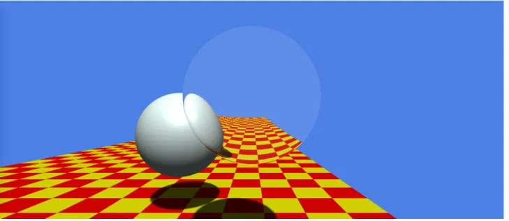
Figure 1: A fake Whitted-style ray tracing scene done with the rasterization pipeline.
a) Look for // TODO: in main.js and reproduce the scene in the constructor() and update() function.
b) What light effects are missing or appear wrong in the reproduced scene (Figure1)? Name three.
However, the Whitted-style ray tracing is still considered wrong and is not compatible with the rendering equation.
1https://www.medien.ifi.lmu.de/lehre/ss20/cg1/demo/7-illumination/whitted/
c) What are the effects that cannot be implemented with Whitted-style ray tracing? Name two.
d) In one sentence: why is Whitted-style ray tracing not compatible with the rendering equation?
Answer text questions in the README.md that comes with the provided code skeleton, then include your answers and implementation in a folder called “task01”. Exclude the installed dependencies (foldernode_modules) in your submission.
Task 2: Monte Carlo Ray Tracing (a.k.a. Path Tracing)
In the lecture, you learned how to calculate the Monte Carlo integration (MCI). For a definite integral Rb
af(x)dx, with the random variable Xk∼p(x), the Monte Carlo estimator is:
1 N
N
X
k=1
f(Xk) p(Xk)
IfXkare unifrom random variables, thenXk∼p(x) = b−a1 , and the Monte Carlo estimator for uniform random variables becomes:
b−a N
N
X
k=1
f(Xk)
Therefore, with Monte Carlo integration, we can write the rendering equation
Lo(x, wo) =Le(x, wo) +Z
Ω
Li(x, wi)fr(x, wi, wo) cosθidwi in a discrete form.
Lo(x, wo) =Le(x, wo) + 1 N
N
X
k=1
Li,k(x, wi,k)fr(x, wi,k, wo,k) cosθi,k p(wi,k)
a) Recall the BRDF of the lambertian material from Assignment 6, what is the rendering equation using Monte Carlo integration on a Lambertian surface?
b) Calculate p(wi,k) for uniform sampling on a hemisphere (hint: consider spherical coordinates).
The rendering equation integrates all possible directions below a hemisphere from a shading point.
The integration can be separated into two parts: direct illumination and indirect illumination. The shading point affected from direct illumination receives its radiance directly from the light source.
c) Let our light source be an rectagular area light with areaS, rewrite the rendering equation that it integrates the radiance and recieves from the light source, i.e. replace the infinitesimal dw by dswheres is a unit direction from light source to the shading point.
Now, for the last task of this course let’s implement a simple path tracer that can render the classic Cornell Box, as shown in Figures2 and 3. An interactive demo can be found online2.
To achieve this goal and by utilizing what you have practiced over the course (three.js with cus- tomized GLSL shaders), we need to construct the code skeleton for this task in a slightly different way than we did it for the other tasks.
In the previous tasks, thethree.js part serves as a renderer for constructing a desired scene graph and eventually uses WebGL APIs to rasterize what you described for the scene graph. However, the
2https://www.medien.ifi.lmu.de/lehre/ss20/cg1/demo/7-illumination/pathtracer/
(a) Direct illumination with no
light bounces. (b) One bounce global illumina-
tion. (c) Two-bounce global illumina-
tion.
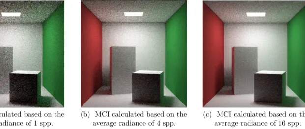
Figure 2: The Cornell Box is rendered by path tracing where the Monte Carlo integration is calculated basd on the average of 20 randomsamples per pixel (20 spp).
(a) MCI calculated based on the
average radiance of 1 spp. (b) MCI calculated based on the
average radiance of 4 spp. (c) MCI calculated based on the average radiance of 16 spp.
Figure 3: The Cornell Box is rendered by path tracing with two light bounces.
rendering pipeline under paradigm of ray tracing is different from rasterization. Thus, in the code skeleton, we use three.jsto create a plane geometry, by using an orthographic projection we make this plane our whole viewport.
As said, with this setting, the plane becomes our viewport, and its material becomes the pixels we are going to program. Therefore, we can fully concentrate on our customized fragment shader to create everything we want to render. Subsequently, for each fragment, we compute the color of a ray in the fragment shader using path tracing.
To make the rendering more interactive, the code skeleton takes into account the number of light bounces and samples per pixel (spp) that we are going to use for the ray bounces while the spp determine the Monte Carlo integration. One can change the values interactively to see how the path tracing is influenced by these two parameters. For instance, Figure2ashows the direct illumination of the Cornell Box where the light has no bounces, Figure 2bshows one bounce global illumination and Figure 2cshows two bounce global illumination; Figure 3a shows the Monte Carlo integration with 1 spp, Figure3b with 4 spp and Figure3c with 16 spp.
d) Use the rendering equation you derived from a), b) and c) and implement Monte Carlo ray tracing in the function vec3 shade(in ray r) in cornellbox.fs.glsl (you don’t need to consider indirect illumination for this implementation).
Hint:
Your implementation should not be longer than 30 lines of code. A pesudocode to better understand how the path tracer works:
1 shade(wo) {
2 Li = 0
3 Lo = 0
4 for i = 0; i < bounces; i++ {
5 if wo not hit the world {
6 return Lo
7 }
8 if wo hit light source {
9 return Lo
10 }
11 Li = Li * hitted material color
12 if light is not blocked in the middle {
13 Lo += radiance at hit position // use the rendering equation
14 }
15 wo = randomly sample one direction
16 }
17 return Lo
18 }
e) What can you conclude when you increase the number of bounces? Will the scene become pure white with infinite light bounces? If yes/no, why? Justify your answer.
f) What can you conclude when you increase the samples per pixel? How much samples per pixel do we need eventually?
Answer text questions in the README.md that comes with the provided code skeleton, then include your answers and implementation in a folder called “task02”. Exclude the installed dependencies (foldernode_modules) in your submission.
Submission
• Participation in the exercises and submission of the weekly exercise sheets is voluntary and not a prerequisite for participation in the exam. However, participation in an exercise is a good preparation for the exam (the content is the content of the lecture and the exercise).
• For non-coding tasks, write your answers in a Markdown file. Markdown is a simple mark-up language that can be learned within a minute. A recommended the Markdown GUI parser is typora (https://typora.io/), it supports parsing embedded formula in a Markdown file. You can find the syntax reference in its Help menu.
• Please submit your solution as a ZIP filevia Uni2Work (https://uni2work.ifi.lmu.de/) before the deadline. We do not accept group submissions.
• Your solution will be corrected before the discussion. Comment your code properly, organize the code well, and make sure your submission is clear because this helps us to provide the best possible feedback.
• If we discover cheating behavior or any kind of fraud in solving the assignments, you will be withdrawn for the entire course! If that happens, you can only rejoin the course next year.
• If you have any questions, please discuss them with your fellow students first. If the problem cannot be resolved, please contact your tutorial tutor or discuss it in our Slack channel.