GEOMAR REPORT
Berichte aus dem GEOMAR
Helmholtz-Zentrum für Ozeanforschung Kiel
Nr. 57 (N. Ser.)
January 2021
Berichte aus dem GEOMAR
Helmholtz-Zentrum für Ozeanforschung Kiel
Nr. 57 (N. Ser.)
January 2021
Deutscher Forschungszentren e.V.
Autor / Author:
Christian Berndt with contributions by Morelia Urlaub, Marion Jegen, Zarah Faghih, Konstantin Reeck, Gesa Franz, Kim Carolin Barnscheidtt, Martin Wollatz-Vogt, Jonas Liebsch, Bettina Schramm, Judith Elger, Michel Kühn, Thomas Müller, Mark Schmidt, Timo Spiegel, Henrike Timm, Anina-Kaja Hinz, Thore Sager, Helene Hilbert, Lea Rohde, Torge Korbjuhn, Silvia Reissmann, Nicolaj Diller
GEOMAR Report
ISSN Nr.. 2193-8113, DOI 10.3289/GEOMAR_REP_NS_57_2021
Helmholtz-Zentrum für Ozeanforschung Kiel / Helmholtz Centre for Ocean Research Kiel GEOMAR
Dienstgebäude Westufer / West Shore Building Düsternbrooker Weg 20
D-24105 Kiel Germany
Helmholtz-Zentrum für Ozeanforschung Kiel / Helmholtz Centre for Ocean Research Kiel GEOMAR
Dienstgebäude Ostufer / East Shore Building Wischhofstr. 1-3
D-24148 Kiel Germany
Tel.: +49 431 600-0 Fax: +49 431 600-2805 www.geomar.de
German Research Centres
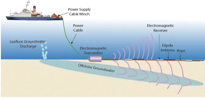
we acquired controlled-source electromagnetic, seismic, hydroacoustic, geochemical, seafloor imagery data off Malta. Preliminary evaluation of the geophysical data show that there are resisitivity anomalies that may represent offshore freshwater aquifers. The absence of evidence for offshore springs means that these aquifers would be confined and that it will be difficult to use them in a sustainable manner. The objective of the second project, MAPACT-ETNA, is to monitor the flank of Etna volcano on Sicily which is slowly deforming seaward. Here, we deployed six seafloor geodesy stations and six ocean bottom seismometers for long-term observation (1-3 years). In addition, we mapped the seafloor off Mt. Etna and off the island of Stromboli to constrain the geological processes that control volcanic flank stability.
1.2 Zusammenfassung
SO277 OMAX diente zwei wissenschaftlichen Projekten. Ziel des ersten Projekts, SMART, war die Entwicklung multidisziplinärer Methoden zur Erkennung, Quantifizierung und Modellierung von Offshore-Grundwasserspeichern in Regionen, die durch Karbonatgeologie geprägt sind, wie z.B. dem Mittelmeerraum. Zu diesem Zweck haben wir vor Malta elektromagnetische, seismische, hydroakustische und geochemische Daten sowie Meeresboden-Videoaufnahmen erfasst. Die vorläufige Auswertung der geophysikalischen Daten zeigt, dass es auf dem Schelf vor Malta elektrische Leitfâhigkeitsanomalien gibt, die auf Süßwasservorkommen hinweisen können. Das Fehlen jeglicher Anzeichen für größere Austritte von Frischwasser am Meeresboden zeigt jedoch, dass diese Grundwasserleiter heutzutage nicht signifikant mit dem meteorischen System in Verbindung stehen und es schwierig sein wird, sie auf nachhaltige Weise zu nutzen. Das Ziel des zweiten Projekts, MAPACT-ETNA, ist die Überwachung der Flanke des Ätna-Vulkans auf Sizilien, der sich langsam seewärts verformt. Hier haben wir sechs Geodäsiestationen und sechs Seismometer am Meeresboden für die Langzeitbeobachtung (1-3 Jahre) installiert. Außerdem haben wir den Meeresboden vor dem Ätna und vor der Insel Stromboli kartiert, um die geologischen Prozesse besser zu verstehen, die die Stabilität von Vulkanflanken mitbestimmen.
2 Participants
2.1 Principal Investigators
Name Institution
Weymer, Bradley, Dr.
Berndt, Christian, Prof.
GEOMAR GEOMAR
Jegen, Marion, Dr.
Schmidt, Mark, Dr.
Haroon, Amir, Dr.
GEOMAR GEOMAR GEOMAR
2.2 Scientific Party
Name Discipline Institution
Berndt, Christian, Prof. Marine Geophysics / Chief Scientist GEOMAR Jegen, Marion, Dr.
Schmidt, Mark, Dr.
Marine Geophysics / Lead EM Marine Geochemistry / Lead Chemist
GEOMAR GEOMAR Urlaub, Morelia, Dr.
Elger, Judith, Dr.
Marine Geology / Lead Geodesy Seismic acquisition
GEOMAR GEOMAR Thomas Müller, Dr.
Schramm, Bettina Petersen, Florian Kühn, Michel Reeck, Konstantin Faghih, Zahra Franz, Gesa Hilbert, Helene Kästner, Felix Sager, Thore Razeghi, Yousef
Barnscheid, Kim Carolin Klein, Johanna
Hinz, Anina-Kaja Timm, Henrike Liebsch, Jonas Spiegel, Timo Wetzel, Gero
Wollatz-Vogt, Martin
Hydrologist / chemist Ocean bottom seismometers Geodesy
Seismic processing EM
EM EM
Watch keeper Watch keeper Watch keeper Watch keeper Watch keeper Watch keeper Watch keeper Watch keeper Watch keeper Geochemistry Seismic engineer EM engineer
GEOMAR GEOMAR GEOMAR GEOMAR GEOMAR GEOMAR GEOMAR GEOMAR GEOMAR GEOMAR GEOMAR GEOMAR GEOMAR GEOMAR GEOMAR GEOMAR GEOMAR GEOMAR GEOMAR
2.3 Participating Institutions
GEOMAR Helmholtz-Zentrum für Ozeanforschung Kiel 3 Research Program
3.1 Description of the Work Areas 3.1.1 The Maltese shelf
Malta is representative for a large part of the Mediterranean coast line, and is also one of the ten poorest countries globally in terms of water resources per inhabitant (Vallée, D. et al. 2003).
Stratigraphically, the islands consist of Oligocene and Miocene limestone formations: from top to bottom Upper Coralline Limestone, Greensand, Blue Clay, Globigerina Limestone and Lower Corraline Limestone. This stratigraphy makes it a type example for the geology in large parts of the Mediterranean. The archipelago hosts an excellent example of an unconfined carbonate rock aquifer onshore in the Lower Coralline Limestone, which is overlain by an aquitard the Globigerina Limestone. This aquitard continues offshore out to the shelf break. Existing borehole data and pockmarks indicate that the groundwater aquifer extends offshore, but so far it is unknown if the underlying aquifer also extends all the way to the shelf break or if it terminates somewhere on the shelf. Because of sea-level rise of 110 m after the last glacial maximum it is likely that the shelf and adjacent seafloor host both recharging and fossil aquifers. Groundwater is known to seep along the coastline and shallow seafloor (Micallef, A. et al. 2013).
3.1.2 The flank of Mt. Etna, Sicily
Mount Etna is Europe’s largest active volcano. It rises to 3330 m above sea level. The volcanic edifice of Etna builds upon continental crust, but about 2/3 of its eastern flank locate under water in the Ionian Sea. The western Ionian Sea is a complex and active tectonic setting. Beside volcanism and flank instability the area is furthermore affected by strong bottom currents and diapirism.
3.1.3 Stromboli
Stromboli volcano is part of the Eolian Island backarc chain in the Tyrrhenian Sea north of Sicily.
The volcano is 926 m above sea level and over 2700 m on average above the sea floor and has
been in almost continuous eruption for the past 2,000–5,000 years. A significant geological feature of the volcano is the Sciara del Fuoco ("stream of fire"), a big horseshoe-shaped depression created in the last 13,000 years by several collapses on the north-western side of the cone (Tibaldi et al.
2009).
3.2 Aims of the Cruise
SO277 contributes to two scientific projects and its agenda developed from the combination of two different ship time proposals: OMAX which was conceived to acquire a comprehensive data set to study freshened groundwater in the frame of the Helmholtz European partnering project SMART and GPF 18-1-89 MAPACT-ETNA (Monitoring and mAPping ACTive deformation of Mount ETNA).
3.2.1 Offshore groundwater
Coastal regions are the most densely-populated areas in the world with an average population density nearly 3 times higher than the global average (Small, C. 2003). Freshwater resources in coastal states and island nations are therefore under enormous stress, and their quantities and qualities are rapidly deteriorating. This problem is exacerbated by population growth, pollution, climate change and political conflicts (Bates, B. 2008). Problems are especially felt in arid areas, such as Malta, where groundwater is the only source of freshwater and the periods of highest demand (e.g., agricultural and tourist seasons) coincide with the periods of lowest recharge from precipitation (Post, V. 2005). By comparison, Cape Town, South Africa is the first major city in the modern era to face the threat of running out of drinking water, and other large cities like Jakarta, and Beijing are likely to follow suit.
Offshore aquifers (OAs) have been proposed as an alternative source of freshwater to cover demand by domestic, agricultural and tourist industries in coastal regions (Bakken, T. H. et al.
2012). During the Last Glacial Maximum (19-22,000 years ago), modern shelf areas were sub- aerially exposed, leading to the development of extensive water tables recharged by atmospheric precipitation (meteoric water), rivers, lakes and, in some areas, glacial meltwater (Burnett, W. et al. 2006). In view of the fact that sea level has been much lower than today for 80% of the Quaternary period (last 2.6 million years), and that meteoric groundwater systems migrate landwards more slowly than rising sea levels, remnants of meteoric groundwater occur extensively offshore (Evans, R. L. 2007). An OA has been defined by (Post, V. E. 2013) “as a groundwater body with a minimum horizontal extent of 10 km, and a minimum concentration of total dissolved solids (TDS) less than 10 g/L, roughly ⅓ the salinity of seawater.” Two types of OAs can be distinguished (Fig. 1). The first type (active) entails a present-day, permeable connection of the OA with a terrestrial aquifer recharged by meteoric water (Bratton, J. F. 2011, Johnston, R. H.
1983). Such aquifers tend to be wedge-shaped, becoming thinner and more saline with increasing
been emplaced by meteoric recharge during lowered sea level periods (Leahy, P. et al. 1982) and that are no longer recharged.
Recent studies have estimated the volume of OAs to range between ~ 3 x 10⁵ km3 (Cohen, D. et al.
2010) and 4.5 x 10⁶ km3 (Adkins, J. F. et al 2002), with a more robust estimate of 5 x 10⁵ km3 (Post, V. E. et al. 2013). The latter is two orders of magnitude greater than what has been extracted globally from continental aquifers since 1900 (4.5 x 10³ km3). The salinity of OAs can range between freshwater and seawater values, and the salinity threshold defined by ( Post, V. E. et al. 2013) corresponds to the upper limit of the salinity range used for the definition of brackish water for desalination (Greenlee, L. F. et al. 2009). Since
submarine groundwater can be exploited using conventional technology from the oil and gas industry and onshore groundwater exploitation, and because the costs seem to be economically competitive with desalination (Bakken, T. H. et al. 2012), OAs have the potential to become an important resource that can relieve water scarcity and mitigate the adverse effects of groundwater depletion (e.g. land subsidence, saltwater intrusion) in densely populated coastal regions.
The characteristics of offshore groundwater systems remain poorly constrained, and there are many first-order questions, related to aquifer geometry and distribution, that need to be addressed.
Conventional offshore groundwater aquifer and submarine groundwater discharge (SGD) methods rely on point-source data from boreholes, seepage meters, and chemical radionuclide tracer techniques that cannot provide continuous information of the groundwater system (Burnett, W. et al. 2006). Additionally, most measurements and research efforts have focused on the nearshore zone (up to several km from the shoreline) (Davidson-Arnott, R. et al. 1999), mainly because of accessibility, the presence of observable discharge at low tides, and its direct association with the unconfined surficial aquifer and topographically driven flow (Bratton, J. F. 2010).
The data to be acquired within this cruise address two of the overarching goals of the SMART project, which are: a) To develop a best practice guide on how to combine geophysical measurements with geochemical characterisation to detect, characterise and monitor OAs, and b) To quantify the hydrologic budget of OAs.
Fig. 3.1 Cartoon depicting the differences between active (connected) and fossil (disconnected) offshore aquifers. The modern day active aquifers are recharged by precipitation (green arrows). Fossil aquifers are no longer fed by meteoric water and are subject to saltwater intrusion (red arrows).
There are two working hypotheses driving the study design
Hypothesis 1: The volume and spatial extent of offshore aquifers in carbonate settings can be determined by integrating seismic and electromagnetic methods
Hypothesis 2: The aquifers off Malta are active systems that discharge into the ocean.
In order to test these hypotheses, we had three research objectives:
Objective 1: Building a geological model and constraining the volume and spatial extent of offshore aquifer(s) by geophysical data acquisition
Terrestrial hydrogeological investigations on Malta define two aquifers: a perched aquifer in the Upper Coralline Limestone (high porosity) and a mean sea-level Ghyben-Herzberg freshwater lens in the Lower Coralline Limestone with lower porosity, separated by an impermeable “Blue Clay”
layer (i.e., Stuart, M. et al. 2010). The study area is located north of the Great Fault in Malta, where all the relevant formations hosting the aquifers occur and where the highest probability that an impermeable layer (Blue Clay) may extend offshore providing a seal for a potential offshore aquifer. The study area includes the widest and most gently sloping part of the Maltese continental shelf and bedrock/outcrop scarcity makes it the most suitable location for bottom towed CSEM experiments. Further indicators of the OA are a series of box canyons that are located upslope of a limestone cliff and are indicative of SGD and observations of flares in sub-bottom profiles reported by Micallef, Berndt and Debono (Micallef, A. et al. 2011). While the OA indications are indirect within the Malta region, extensive groundwater seeps have been located offshore in very similar geological settings, particularly offshore Sicily and the Levant (Bakalowicz, M. 2018). To achieve a focus on the region of interest, in October, 2018 we conducted marine 2D seismic and CSEM measurements extending the land EM profiles offshore east of the island on the R/V Hercules within the framework of the MARCAN project led by co-proponent Aaron Micallef.
Terrestrial EM measurements were collected in July, 2018 by colleagues at UoM, and Texas A&M University.
We have conducted two types of seismic experiments. First, we collected 2D seismic data using the P-Cable system in 2D mode. The 2D seismic lines from the area between Malta and Gozo into the offshore study area allow us to correlate information from the boreholes.
Apart from mapping the stratigraphic changes, which are often associated with porosity changes, the move-out characteristics of the 2D seismic data and ocean bottom seismometer data will allow us to determine seismic velocities that provide rough porosity estimates and crucially show variations in petrophysical parameters away from the boreholes.
The second experiment was the collection of a high-resolution 3D seismic cube. The aim of this experiment was to image the entire subsurface in three dimensions. This will provide information on the geological variations such as faults, stratigraphic terminations, etc. that are crucial for building the hydrological models and constrain the geology for the inversion of the CSEM data.
The cube includes the shelf break, i.e. across the area that was subaerially exposed during the sea- level lowstand during the last glacial maximum (LGM) and the area that was always submerged.
CSEM electromagnetic data were collected along profiles covering the seismic 2D profiles as well as 3D seismic cube. CSEM and seismic 3D cube lines as well as 2D regional seismic lines will be co-rendered to investigate first order correlation between resistivity changes and positions of
Objective 2: Localize seep structures, which open a window into the aquifer at depth, using high resolution AUV based photo imagery, water column sensors and Parasound data.
In order to understand the functioning of the aquifer and to direct seep sampling (Aim 3) it is necessary to localize groundwater seeps. In spite of extensive efforts using the video-CTD casts, gravity cores and AUV imagery it was not possible to discover any groundwater seeps.
Objective 3: Characterize seeping groundwater to be able to interpret the geophysical data and provide background information for the hydrogeological models such as mixing, regional fluid flow rates, and age of the groundwater in the distal parts of the aquifer
In the absence of seep sites it was not possible to obtain direct samples of offshore groundwater.
Although much of the geochemical data still awaits analysis the comprehensive studies did not show signs of groundwater seepage. This would falsify the second hypothesis that the aquifers are connected to the ocean and suggests that the groundwater system off Malta is most probably a fossil system.
3.2.2 Slope stability of volcanic islands
Volcanoes are among the most rapidly growing geological structures on Earth. Consequently, volcanoes commonly suffer structural instability that may result in lateral flank collapses, such as the 1980 Mt St Helens collapse. Collapses of ocean island volcanoes or those along shorelines can trigger ocean-wide tsunamis with extreme effects. The world just witnessed a small example of such an event: the 22 December 2018 collapse of Anak-Krakatau in Indonesia that caused a tsunami with 430 fatalities at the surrounding coasts (Walter et al. 2019). Volcanic flank instability is a global and widespread phenomenon, and varying degrees of flank instability have been reported from all scales of volcanoes, such as Kilauea (Hawaii), the Canary Islands, Galapagos, and Tristan da Cunha (Poland et al. 2017).
Mount Etna, located on the coast of Sicily (Italy), is a basaltic stratovolcano located at the edge of the Calabria-Tyrrhenian slab. Right-lateral transtension between two slabs produce a vertical ‘slab window’, which allow magma to upwell. Mount Etna is oone of the most intensively monitored
and best studied volcanoes in the world. Repeated and ongoing GPS campaigns, permanent GPS monitoring onshore, and interferometric synthetic aperture radar (InSAR) data provide evidence for downward movement of the eastern and south-eastern flanks coupled with overall flank subsidence (e.g. Bonforte et al. 2011, Palano 2016). In contrast, the western flank is apparently more stable with no or only minor movement (e.g. Puglisi et al. 2001). Seaward motion of Mount Etna´s southeastern flank manifests in continuous deformation as well as episodic ‘slow slip’
events that are aseismic and occur irrespective of volcanic activity (Palano 2016). Hence, displacement rates are highly variable over time, resulting in about 30-50 mm/year. Whereas vertical ground deformation due to magma overpressure reaches a maximum at the volcano summit, flank subsidence and seaward movement concentrates along the coast (Bonforte et al.
2011).
Large parts of Mount Etna’s eastern part are covered by water, so that traditional geodetic measurements, such as those by GPS or InSAR, cannot be applied due to the opacity of seawater to electromagnetic waves. Consequently, offshore slip is highly unconstrained, resulting in high uncertainties in models that seek to fit the onshore GPS data. Hypotheses that attempt to explain Mount Etna’s flank instability include the weight of the volcanic pile, increase of magma pressure (Borgia et al. 1992), a weak substrate (Nicolosi et al 2014), combined magmatic inflation and continental margin instability (Chiocci et al. 2011), or a combined volcano edifice and continental margin instability (Gross et al. 2016). The disagreement on the causes of flank instability mainly originates from the lack of information on the dynamics of the submerged part of the volcano.
Between 2016 and 2018, an acoustic telemetry network measured displacement of the submerged unstable flank at one location. The network recorded a minimum of 4 cm of slip during an eight- day sliding event in May 2017, while displacement on land peaked at ~4 cm at the coast. Such large deformation away from the magmatic system can only be explained by a gravitational effect that is further destabilized by magma dynamics (Urlaub et al. 2018). However, the observation period is less than two years and it is impossible to deduce long-term rates.
The spatial outline of the unstable flank is well defined onshore by geodetic, geophysical, and geological methods (e.g. Bonforte et al. 2011). Along the northern boundary of the unstable flank,
Fig. 3.2 Shaded relief map of Etna’s eastern flank (grey: onshore, coloured: offshore) with the main faults that are kinematically related to seawards sliding of the volcano’s unstable eastern flank (Urlaub et al. 2018).
of both onshore fault systems, likely represents the southern boundary (Chiocci et al. 2011, Gross et al. 2016, Urlaub et al. 2018). Based on bathymetric and seismic data, Gutscher et al. (2016) speculate that this fault is further connected to a regional crustal structure; the North Alfeo Fault.
According to Gutscher et al. (2016, 2017) the North Alfeo Fault is the surface expression of an active slab tear. The eastern and most distal end of the flank is less clear. A compressive feature might be expected. One candidate could be a plateau about 40 km off the coast, where seismic data indicates active uplift. This structure has been interpreted as a serpentinite diapir by others (Polonia et al. 2017).
Stromboli volcano has experienced two major eruptions in 2019. The eruptions were accompanied by strong ground deformation, landslides and large pyroclastic flows that entered the sea at the northwestern flank. While satellite imaging reveals morphological changes of the subaerial flank, changes at the seafloor remain hidden. Information on the distribution and the type of volcanic deposition will provide valuable insights into the growth of island volcanoes and the results will inform the analysis of potential weakness zones in volcanic edifices such as the flank of Mt. Etna.
Objectives
The first objective of GPF 18-1-89, side user on cruise SO277, was to install an autonomous seafloor geodetic array to understand deformation of Mount Etna’s submerged flank over long terms. Our successful previous monitoring campaign (Urlaub et al. 2018) proved that (i) the technique is well suited to monitor unstable volcanic flanks under water, (ii) the location of the array coincides with the boundary of the unstable flank, (iii) the array design is ideal for monitoring flank instability, and (iv) the slip lies well within the resolution of the array. It is now important to analyse the displacement trend over long-terms (years to decades). In order to evaluate the hazard from a potential flank collapse it is crucial to know if the unstable flank is accelerating or decelerating.
The second objective is to collect high-resolution multibeam and Parasound data to identify if the active fault partitions into multiple faults in the landward direction and if it is linked to regional tectonic structures. If Mount Etna’s unstable flank was connected to a deep, large-scale tectonic structure, its instability could in parts be controlled by the regional tectonic setting. A connection is not fully recognizable from existing bathymetric data with a grid spacing of 30 m (<1000 m water depth) and 100 m (>1000 m water depth). It could, however, be recognizable in multibeam data collected during dedicated surveys with the shipboard system.
The third objective is to map the distribution of the volcanic deposits associated with the 2019 eruptions at Stromboli. This is a unique opportunity because Italian colleagues have carried out a similar bathymetric survey of the flank of Mt. Stromboli in 2016 (Casalbore, pers. comm.). By calculating the difference between that data and our new data we will be able to identify the nature
and distribution of volcanic deposits associated to the recent eruptions. These changes could include traces of pyroclastic flows, landslide scars, landslide blocks, all of which could have formed due to the recent major eruptions.
3.3 Agenda of the Cruise
The coronavirus situation in Germany required that three planned legs had to be combined: the two legs of Meteor cruise M170 that were originally scheduled to take place in December 2020 and parts of a Poseidon cruise that was already split up into Alkor cruise AL532 and Meteor cruise M169. The combination of these cruises and the reduced capacity to carry scientists meant that the work program had to be reduced by omitting the ROV that was planned for M170/2 and by reducing the capacity for geochemical analyses on board.
Sailing from Emden and back meant two long transits of eleven days each. The work was split into four packages. First, we deployed marine geodesy stations off Mt. Etna. Then we carried out the bulk of the work off the Maltese Islands before returning to Mt. Etna to double-check that the geodesy stations were operating properly and deploy six long-term ocean bottom seismometers.
Finally, we used the remaining day of ship time that was saved for fixing the geodesy stations in case of problems to map the recent volcanic deposits off Stromboli a study that also addresses volcano flank stability.
4 Narrative of the Cruise
All times in the narrative are local times.
Monday, 14.8.2020
We departed from Emden at noon and started our long transit to Italy. Fortunately, the weather was fine for the entire transit allowing us to sail with 12 rather than the expect 11 knots which meant that we gained one day for work in the study area.
Fig. 2.3 Track chart of R/V SONNE
CRUISE SO277.
Bathymetry from Smith and Sandwell (1997). The three main working areas are labeled.
transit to the first study area off Mt. Etna passing through the Strait of Messina in the early evening.
Monday, 24.8.2020
We arrived in the study area off Catania at midnight and conducted a CTD cast that lasted until 07:00 in the morning. Apart from measuring the CTD profile we also used the video camera to obtain seafloor images in the area where the geodesy stations had to be deployed. The seafloor was covered with marine muds and showed abundant bioturbation but no clear signs of tectonic deformation. At 08:00 we began with the deployment of two geodesy stations which was completed by 15:00. While progressing to the first multi-beam line we spotted a bright red item at the location of the first deployment site. Concerned that one of the geodesy stations might have surfaced accidentally, we returned back only to find a bright red fairground balloon that was swimming in the water. Having sailed back to the deployment site, we made most of the opportunity and connected to both stations to check that they were operating properly before commencing with a multi-beam survey of Etna’s flank during the night.
Tuesday, 25.8.2020
With a fresh northerly breeze, we continued to deploy the seafloor geodesy stations. The work progressed exceptionally well and we managed to place the remaining four stations on the seabed between 8:00 in the morning and 17:00. Afterwards, we continued to collect multi-beam data over the lower slope of Mount Etna.
Wednesday, 26.8.2020
In the morning at 08:00, we returned to the geodesy stations and communicated with them to ascertain that all were functioning properly. After we were satisfied that this was the case and that they could all range each other, we started our transit to the next study area off Malta. Initially we collected multi-beam data along the Malta Escarpment until we reached the boundary of our permitted work area. We arrived off Malta shortly before midnight.
Thursday, 27.8.2020
We started with a first CTD cast off Gozo to obtain a sound velocity profile for the calibration of the hydro-acoustic systems and to collect background water samples for the geochemistry.
Afterwards until 07:00, we did a Video-CTD transect closer to the coast off the eastern tip of Gozo.
At 08:00 we deployed the AUV off St. Paul’s Bay and conducted a video survey of the seafloor in an area known for gas seepage. At 14:00 we retrieved the AUV and started to deploy 9 OBEMs until 19:00, then 10 OBS until 23:00. Afterwards, we carried out a multi-beam survey throughout the night.
Friday, 28.8.2020
We completed the multi-beam survey at 09:00 and started to deploy the 2D seismic system off Camino at 10:00. The system was up and running at 10:45, but after half an hour a fishing line got entangled and we had to retrieve the streamer to unhook it. From 13:00 onwards we acquired 2D seismic lines off the central and eastern parts of Malta.
Saturday, 29.8.2020
In fine weather we continued the 2D seismic data acquisition without further interruptions.
Sunday, 30.8.2020
In fine weather we continued the 2D seismic data acquisition.
Monday, 31.8.2020
In fine weather we continued the 2D seismic data acquisition.
Tuesday, 1.9.2020
We continued collecting 2D seismic data until 10:00 when the tow cable of the streamer started to show signs of malfunctioning. We retrieved the streamer and continued shooting into the OBS until 15:30. We then took on board the seismic source. Afterwards, we retrieved the two outermost OBS that were carrying the experimental mini-OBS because their batteries only last for five days.
We also deployed three more OBEM in the study area off Gozo. Afterwards, we started a multi- beam survey beyond the shelf edge to ascertain that there are no obstacles for the CSEM tow that was planned for the following day.
Wednesday, 2.9.2020
At 08:00 we deployed the CSEM system and towed it along a track below and parallel to the escarpment along the NE coast of Gozo. Unfortunately, only the first two of the four receivers logged data but those are of good quality.
Thursday, 3.9.2020
We recovered the CSEM system between 07:00 and 09:00 in the morning. Interestingly, two pieces of slate were stuck to the depressor (pig) suggesting that the slates that are known to exist below the lower coralline limestone could be outcropping somewhere in the area. Afterwards we surveyed a video CTD track down the shelf edge across a phase reversal in the seismic data and crossing the CSEM line that was acquired in the night before. There were no signs of fluid escape along this track and the entire seafloor including the escarpment that forms the shelf edge turned out to be covered with soft sediment. Originally, we had planned to deploy the AUV in the morning but sometime between the previous AUV deployment on the 27.8. and the 3.9. the container that holds the AUV USBL modem must have opened and the transponder was lost. From 14:00 onwards we deployed the P-Cable 3D seismic system which was operational at 15:30 and we started to acquire 3D seismic data.
Friday, 4.9.2020
In spite of a fresh easterly breeze the P-Cable system was operating fine until one of the air pipes of the seismic source came loose and we had to take the source on board for repairs at 11:00.
The system was back in operation at 14:00 and we continued acquisition of 3D seismic data.
We finished the planned P-Cable lines at 10:00 in the morning. Afterwards we began to acquire data in the numerous gaps caused by avoidance of fishing gear. At 17:00 a fishing line with hooks got entangled in the segment between streamer 11 and 12 and damaged the cross-cable segment and the T-junction. The port side paravane and streamers 11 to 16 had to be taken onboard and the cross-cable segment had to be replaced. Afterwards we continued filling the gaps in the P-Cable cube.
Tuesday, 8.9.2020
P-Cable acquisition finished at 14:30 in spite of some remaining holes in the fold map. These could not be filled because of fishing gear that was floating permanently at those locations. The system was back on board and the back deck was set up for CSEM operations. The CSEM system was deployed until 17:00 and we collected another CSEM profile beyond the shelf edge.
Wednesday, 9.9.2020
We recovered the CSEM system until 09:30 in the morning. The system was working well and all receivers collected data. At 10:30 we deployed the AUV close to Gozo and then started a first video-CTD transect near Sikka-i-Bajda reef. This was completed at 16:00 when we returned to the AUV station and retrieved the vehicle. We then started a second video-CTD transect at the pockmark field east off Gozo. Within the pockmarks the water was more turbid but no signs of fluid escape could be found. The station was finished at 22:00 and we collected several parallel Parasound profiles on the shelf to ascertain that there are no obstacles for the CSEM track planned for the next day.
Thursday, 10.9.2020
At 08:00 we started to recover four of the OBEM receivers. This was finished successfully by 11:00. Afterwards we conducted two CTD transects in the east and north off Gozo. During the first dive we could see the water column imaging anomaly east off Comino, but we could not detect a signal in the CTD or the other sensors. The second site confirmed the impression that the pockmarks below the shelf break are not active. At 16:00 we redeployed the CSEM system for another transect east off Gozo.
Friday, 11.9.2020
The CSEM transect was finished at 04:30 and the system was recovered until 06:30. Afterwards we steamed to the meeting point off Comino to take onboard the spare USBL modem for the AUV.
This was delivered by boat at 09:00. From 10:00 to 11:30 we deployed four OBEM on a transect off northern Malta and the Comino channel and from lunch time to 16:00 we collected the first gravity cores. The first core consisted of fine sands and carbonate debris and it was possible to
centrifuge pore water. At the other two coring sites there was no penetration but some carbonate debris in the core catcher. During the night we conducted another CSEM tow north off Gozo.
Saturday, 12.9.2020
The CSEM system was successfully recovered in the morning and at 08:30 we deployed the AUV at the most prominent water column imaging anomaly southeast off Comino. Afterwards we collected three more gravity cores north off Gozo with mixed success before recovering the AUV at 14:00. Afterwards we retrieved the eight OBS and throughout the night we collected Parasound data to survey the track of the next CSEM deployment.
Sunday, 13.9.2020
At 10:00 we met with Dr. Owen Bonicci, the Maltese Minister of Education, who came out to visit us on a pilot boat. He was accompanied by Prof. Aaron Micallef and Dr. Axel Steuwer the University of Malta’s vice rector. Because of coronavirus it was not possible for them to come onboard R/V Sonne but it was possible to exchange presents and talk over the side of the ship.
Afterwards they stayed on to witness the deployment of the video CTD at the site of the most prominent water column anomaly that was identified in the multi-beam data.
When a violent thunderstorm came up, they left back for the harbor. The thunderstorm delayed the following AUV deployment until 14:00 because it was not safe to work on deck. The AUV carried out a short 1.5 hour-dive at the easternmost of the water column anomalies and from 16:00 onwards we began to acquire the next CSEM profile east off Sikka I Bajda reef.
Monday, 14.9.2020
We recovered the CSEM from 06:00 to 08:00. Although the Parasound profile had suggested that there was sufficient sediment cover along the track signs of wear and tear indicated the presence of several hard rock outcrops along the track and one receiver was damaged. From 08:00 to 10:30 we collected more Parasound data off the eastern tip of Malta to find out if another CSEM profile was possible in that region. Unfortunately, it also turned out to be too rough. We discovered, however, several water column anomalies in this area that indicate gas emissions from the seafloor. From 11:00 onwards we conducted three video-CTD casts at sites off eastern Malta where water column anomalies were reported previously. The first site turned out to be an unknown wreck in 118 m water depth. The other two sites did not show signs of fluid seepage either. From 19:00 onwards, we collected multibeam bathymetry data off Comino in extension of Markan CSEM profile 2 as a pre-survey for the final CSEM line.
Tuesday, 15.9.2020
In the morning at 08:00, we deployed the AUV at the northern water column anomaly off Comino in spite of a strong breeze (force 6-7). From 10:00 to 14:30 we collected three gravity cores further north before recovering the AUV at 15:30. The gravity cores showed mainly hemi- pelagic mud, but no evidence for methane in the sediments, authigenic carbonates but fragments of limestones. Afterwards we deployed the EM system in MMR mode (vertical dipole) that allows to tow the system also in rocky areas, but without a receiver. These signals were recorded by the OBEM.
Thursday, 17.9.2020
From 08:00 onwards we collected two video-CTDs at an enigmatic mound NE off Malta that consists of carbonate rocks above the post Messinian soft sediments and at the flare site investigated with the AUV on the day before. With force 7 winds it was not possible to use the AUV. In the afternoon, we took one more gravity core from a box canyon NE of Gozo, before we deployed the CSEM system to acquire electrical resistivity data further offshore.
Friday, 18.9.2020
The windy conditions persisted during the day. At 08:00 in the morning, we recovered the CSEM system which was on deck by 09:30. Afterwards, we collected the twelve OBEM receivers.
This was completed by 16:00. All instruments were safely retrieved and found to have recorded data, although one of the twelve data loggers had stopped after four days. In the evening, we conducted a final video-CTD cast at the southern water column anomaly off Comino before we left the study are to sail back to Sicily.
Saturday, 19.9.2020
We arrived off Mt. Etna in the early morning and set up communication with the seafloor geodesy stations. After we had downloaded the data from the past four weeks since their deployment and had ascertained that they were working correctly, we conducted one video-CTD dive near the geodesy array to see if there are obvious signs of flank deformation across the fault system, but apart from some elongate seafloor discolorations we could not find any anomalies. At 13:00 we started to deploy six ocean bottom seismometers which will stay in the area for one year to measure seismicity in the vicinity of the seafloor geodesy stations. This was completed by 16:00.
Afterwards, we carried out a second video-CTD cast further down along the fault system in about 2000 m water depth. Towards the end of this dive we found signs of chemosynthetic ecosystems that were not expected. Analysis of the water samples will reveal the driving process for the associated fluid seepage. During the night we collected more multi-beam bathymetry data on this part of the slope.
Sunday, 20.9.2020
We continued multibeam surveying until 08:00 in the morning. Then we left the study area to proceed to our final study site off Stromboli. We arrived there at 15:00 and carried out a CTD cast.
Afterwards, we started to survey the western flank of Stromboli using the multi-beam echosounder to image the recent deposits from Sciara del Fuoco.
Monday, 21.9.2020
The multi-beam survey and the scientific program were completed at 20:00 and we started the transit back to Emden.
Saturday, 3.10.2020
We arrived in Emden at 11:00.
5 Preliminary Results
5.1 Hydroacoustic methods (M. Urlaub)
GEOMAR
During SO277 we used three types of hydroacoustic methods: multibeam echosounders, sediment echosounder (PARASOUND) and marine geodetic measurements. These are grouped under hydroacoustic methods, but we discuss the instrumentations, processing, preliminary results individually.
5.1.1 Multi-beam bathymetry
5.1.1.1 Instrumentation
Kongsberg multibeam echosounder systems are permanently installed on RV SONNE; the EM122 for full ocean depth and the EM710 system with a maximum acquisition depth of approximately 2000 m according to the manufacturer’s data. In the working area off Malta with water depths
<200 m only the EM710 was used. In the working areas off Sicily both systems were used in water depths <1400 m, while only the EM122 was used in greater depths. Altogether both systems recorded more than 700 million soundings during SO277.
In addition to bathymetric information the EM122 and the EM710 system register the amplitude of each beam reflection. The amplitude signals correspond to the intensity of the echo received at each beam. It is registered as the logarithm of the ratio between the intensity of the received signal and the intensity of the output signal, which results in negative decibel values. Both systems also allow recording the entire water column. The water column data correspond to the intensity of the echoes recorded from the instant the output signal is produced. All echoes coming from the water column, the seabed and even below the seabed are recorded for each beam. The water column data were stored in separate *.wcd files.
Both the EM122 and EM710 systems apply beam focusing to both transmit and receive beams in order to obtain the maximum resolution also inside the acoustic near-field. The systems are capable of producing more than one sounding per beam (so-called high density mode), such that the horizontal resolution is increased and is almost constant over the whole swath. In multiping mode, two swaths are generated per ping cycle, i.e. one beam is slightly tilted forward and the second ping slightly tilted towards the aft of the vessel, resulting in double the amount of soundings. As a
consequence, both systems achieve a footprint of 0.5° across cruise direction and 1° in cruise direction. High-density equidistant and multiping modes were used and the Frequency Modulated chirp transmit pulse was selected throughout cruise SO277 for both systems.
Positioning is implemented onboard RV Sonne with conventional GPS/GLONASS plus differential GPS (DGPS) by using either DGPS satellites or DGPS land stations resulting in quasi- permanent DGPS positioning of the vessel. The operator station with the Seafloor Information Sytem (SIS) acquisition software receives these signals. Ship motion and heading are compensated within the Seapath and SIS by using a Kongsberg MRU 5+ motion sensor.
Kongsberg EM710
The high-resolution shallow water multibeam echosounder transmits signals in the 70-100 kHz range. The system generates 256 beams providing 400 soundings. In multiping mode a maximum of 800 soundings per ping can be generated. The transmit fan is divided into three sectors to maximize range capability, but also to suppress interference from multiples of strong bottom echoes. The sectors are transmitted sequentially within each ping, and use distinct frequencies or waveforms. The maximum opening angle is 140°. In the working area off Malta the maximum ping frequency was reduced to 2 Hz to avoid persistent freezing of the SIS software. During SO277 the EM710 generally delivered high-quality data between 20 m to approximately 1400 m water depth and worked reliably. In turns, even in minor curves, a clear discrepancy in the quality between inner and outer beams became visible (Fig. 5.1). In areas of little topography the system produced a comparatively high number of erroneous soundings (Fig. 5.1).
Kongsberg EM122
The 12 kHz deep water multibeam echosounder generates 288 beams, resulting in 432 soundings per swath. In multi-ping mode, up to 864 soundings can be generated. The maximum opening angle is 150° and was chosen according to the needs of individual surveys. The EM 122 transducers are modular linear arrays in a Mills cross configuration. Beam inclination was set to automatic. The system provided high-quality data in the deep-water working areas off Sicily and worked without the need of user intervention.
Fig. 5.1 Screenshots from Qimera showing the offset between outer and inner beams of the EM710 system in curves (left) and noise in EM710 data in areas with little topography (right).
Sound velocity probes
Beamforming requires sound speed data at the transducer head, which is available from a Valeport MODUS SVS sound velocity probe. The probe is located in centre of the vessel below the keel, and hence in the direct vicinity of the transducers. This signal goes directly into the SIS operator station. On 10 September 2020 the probe was removed because the adapter plate was needed for other operations. For the rest of the cruise the AML Oceanographic MicroX SV sound velocity sensor, which is part of the thermosalinograph (Self-cleaning Monitoring Box, SMB), provided the sound speed data for the SIS.
Vertical sound velocity profiles were calculated from Video-CTD measurements following Wilson (1960). The sound velocity profile was updated each time a Video-CTD had been deployed.
Because of deep water the sound velocity profiles off Sicily show little variability (Fig. 5.2). On the other hand, large variations in sound velocity were observed in the working area off Malta (Fig. 6). These variations are most likely combined effects of water column mixing by waves, diurnal variations, and internal currents owing to the shallow water environment.
5.1.1.2 Post processing
For multibeam post-processing and visualisation we used the software Qimera developed by QPS hydrographic and marine software solutions (http://www.qps.nl/display/main/home). When loading data from Kongsberg systems into Qimera, the software checks the detection class show flag to determine if soundings are accepted or rejected. Class 8 will always be rejected by default, as recommended by the manufacturer. Qimera then launches any required processing and applies
Fig. 3.2 Sound velocity profiles off Sicily in the Etna (blue, red) and Stromboli (orange) areas calculated from CTD data.
Fig. 5.3 Sound velocity profiles off Malta from CTD data.
to the backscatter data before outputting a georeferenced mosaic.
The software FMMidwater reads, converts, and displays water column data. For fast screening of large data sets we converted the data using a data point reduction factor of 16 or 32 and visually inspected the lines in the stack view. Lines with clear water column anomalies were converted at higher resolution and analysed in detail.
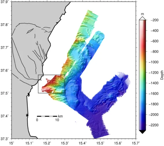
5.1.1.3 Preliminary results Etna
We conducted one dedicated multibeam survey and additionally recorded during transits between stations as well as on the transit to Malta using the EM122 system in water depths of 1000-2300 m and delivered a grid spacing of 30 m (Fig. 5.3). The first survey with EM710 and EM122 in 600-1200 m water depth covered Catania Canyon and the lineament north of it. The survey’s target was to maximise horizontal resolution. Hence, the opening angle of both systems was 90° and the
Fig. 5.4 Bathymetric map of the Catania Canyon and the lineament north of it.
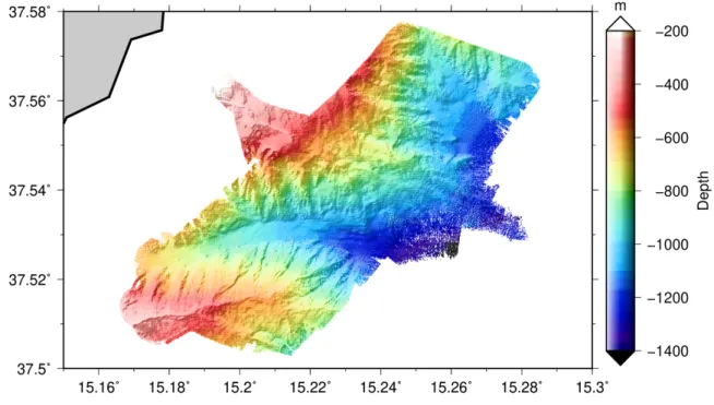
survey was designed to ensure a swath overlap of neighbouring profiles of at least 75%. After post- processing the data was gridded at 10 m spacing (Fig. 5.5).
The data collected during SO277 provides an improved seafloor map with respect to previous bathymetric data, in particular along the North Alfeo Fault, Catania Canyon, and the lineament north of Catania Canyon (Fig. 5.5). The fault trace comes out clearly and smaller-scale features, such as previously unrecognised en-echelon structures or landslide scars show up. The water column data does not yield evidence for any anomalies.
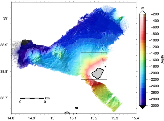
Stromboli
To map Stromboli’s very steep northwestern flank the vessel followed slope-parallel profile lines from 200 m to 3000 m water depth. The opening angles of both the EM122 and EM710 systems were set to maximum on the shallow side and to 45° on the deep side and changed with each turn.
The achieved grid spacing is 30 m for the entire survey with the EM122 system (Fig. 5.6) and 20 m for the depth range 200 – 1500 m with the EM710 system (Fig. 5.7).
Fig. 5.5 Detailed bathymetric map of the selected area in the previous figure.
Fig. 5.6 Shaded relief map of the seafloor around Stromboli and parts of Stromboli channel from the EM122 system (30 m grid spacing).
Fig. 5.7 Shaded relief map of the proximal area of Stromboli’s northwestern flank recorded with the EM710 system (20 m grid spacing).
Malta
The area north-east of the Maltese Islands was the main target area of cruise SO277. This area has been mapped partly in great detail due to multiple overlaps of adjacent tracks and several dedicated multibeam surveys (Table 3). The water depth in the area ranged from 20 to 200 m, with an exception in the northwestern survey area, where water depths reach almost 500 m (Fig. 5.9).
Overall grid spacing is 6 m with better resolution in areas of dedicated surveys.
Table 5.1 Multibeam surveys of SO277
Date File numbers Remarks
Survey NE Malta 27/28 Aug 2020 52-70
2D seismic profiling 71-385
P-cable survey 385-532
CSEM reconnaissance 10 Sep 2020 535-553 CSEM reconnaissance 12 Sep 2020 560-582 CSEM reconnaissance 14 Sep 2020 583-595
CSEM reconnaissance 15 Sep 2020 597-630 Windy, 3-4 m swell
Survey SE Malta 16/17 Sep 2020 643-672 System failure multiple times
Fig. 5.9 Shaded relief map of the entire bathymetric data set collected with the EM710 system in the working area northeast of Malta during SO277. The green line shows the location of the downslope profile in Fig. 5.10. The dashed box shows the location of the backscatter image in Fig. 5.12.
The seafloor seawards of the shelf edge reveals tectonic, sedimentary, bottom current induced, and anthropogenic seafloor patterns. In the northwest a near-vertical, up to 250 m high scarp is prominent. A field of sediment waves of different shapes and sizes stretches out east of Comino.
The new bathymetry also shows circular depressions in an area where pockmarks have previously been identified in side scan sonar data. We also note a singular block surrounded by smooth seafloor topography.
The water column images were analysed for anomalies in the water column that are caused by gas rising up from the seafloor. Gas pathways might also provide pathways for groundwater. The water column images showed several anomalies of varying shapes, sizes, and abundances (Fig. 5.11).
Fish bladders have similar sizes as gas bubbles and therefore cause similar water column anomalies, making them hard to distinguish.
The backscatter data (Fig. 5.12) shows a clear difference in intensities between the shelf and the sedimentary basin. The shelf is predominantly made of hard grounds with high backscatter intensity. This is in contrast to the sedimentary basin with predominantly soft seafloor sediments.
Fig. 5.10 Typical transect crossing the shelf to the sedimentary basin in the northeast of the Maltese Islands (for location see green line in Fig. 5.9).
Fig. 5.11 Screenshots from the FMMidwater software showing examples of water column anomalies in the southeast of Comino. a) Stacked fans along the ship’s track and b) water column image of one ping. The white line in a) indicates the location of the ping.
In the area to the southeast of Malta the backscatter image shows circular structures of notably higher backscatter intensity than the surrounding seafloor. The circles have diameters of about 100 m and show up as very minor positive relief in the bathymetry data. In this area the water column images suggest the presence of multiple flares.
5.1.2 Parasound
5.1.2.1 Method
RV Sonne is equipped with an Atlas Parasound DS P-70 parametric deep-sea sediment echosounder for full ocean depth. The system is a narrow beam sediment echosounder (opening angle 4.5° x 5.0°) that utilises the so-called parametric effect to generate a very low frequency secondary signal by emitting two primary signals of higher frequencies. The Parasound system transmits two independent pulse-modulated harmonic signals via the same transducer array. To generate and utilise the parameteric effect these signals must be generated with extremely high amplitudes. At such signal levels the seawater does not only serve as a propagation medium for the original signals but also generates additional new signal components at different frequencies.
During SO277 the primary frequencies were 18 kHz and 22 kHz. The resulting secondary frequencies are 4 kHz and 40 kHz. For sediment penetration in particular the secondary low frequency is of interest.
Fig. 5.12 Backscatter image of the shelf east of Malta. Light colours are high backscatter amplitudes, representing harder material on the seafloor. For location see Fig.
5.9.
5.1.2.2 Parameter settings
In the deep-water settings at Etna and Stromboli as well as during the transit from Etna to Malta the Parasound system transmitted in a quasi-equidistant transmission sequence with a time interval of 1200 ms. In the working area off Malta the system emitted a rectangular frequency modulated single pulse. The receiver band width for both high frequencies was 66 % and for both low frequencies 33% of the output sample rate (12.2 kHz). The sound velocity was manually set to 1500 m/s.
5.1.2.3 Processing
All raw data were stored in the ASD data format (Atlas Hydrographic), which contains the data of the full water column of each ping for all four frequencies as well as the full set of system parameters. Additionally, a 200 m-long reception window centred on the seafloor of the primary high and the secondary low frequencies was recorded in the compressed PS3 data format after resampling the signal back at 12.1 kHz. This format is in wide usage in the PARASOUND user community and the limited reception window provides a detailed view of subbottom structures.
All data were converted to SEG-Y format during the cruise using the software package ps32sgy version 15.9 (Hanno Keil, Uni Bremen). The software re-fits the different time windows, allows generation of one SEG-Y file for longer time periods, frequency filtering (low cut 2 kHz, high cut 6 kHz, two iterations), and the subtraction of mean. In this format the seismic interpretation software IHS Kingdom can easily read and display the parasound data.
5.1.2.4 Preliminary results
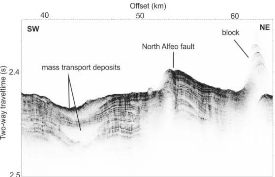
During SO277 we collected approximately 900 km of Parasound profiles. Technical problems did not occur. Imaging the sub-seafloor in volcanic areas was difficult due to steep slopes and hard sediments. Away from the continental slope of eastern Sicily penetration improved greatly. Several profiles cross the North Alfeo fault and document an active tectonic structure (Fig. 5.13).
Fig. 5.13 Parasound profile cutting the North Alfeo fault at an almost vertical angle.
In the Malta survey area the Parasound was mainly used for reconnaissance surveys for gravity coring and CSEM profiles. At the shelf almost all energy was reflected by the hard ground (Fig.
5.13). Penetration was slightly increased for channels cutting through the shelf and improved significantly seawards of the shelf edge.
Carbonates outcropping on the Maltese islands form the acoustic basement in the shelf area. A thin layer of sediments (<3 m) appears to cover the hard carbonates. Seawards of the shelf edge the Parasound data image a body with faint internal reflectors on top of the acoustic basement. We interpret this body as having formed by bottom current activity. Seawards of the sediment body a sequence of stratified sediments cover the acoustic basement. The sediment package is 0.05 s thick next to the drift body and thickens in the seaward direction. The sediment layers change their dip direction, with the two packages being separated by an erosional surface (Fig. 5.14).
The Parasound profiles also provide evidence for fluid escape structures in the sediments seawards of the shelf edge. Fig. 5.15 shows one example of a circular seafloor depression inside the P-Cable area. However, a flare was visible neither in the secondary low nor in the primary high frequencies.
A later visit with the Video CTD did not return any active venting neither.
Fig. 5.14 Parasound profile inside the P-cable cube crossing the shelf, the sediment body adjacent to the shelf edge, and the sedimentary basin. Note that the transect cuts the shelf edge at a small angle.
Fig. 5.15 Parasound profile across a circular seafloor depression.
5.1.3 Seafloor geodesy
5.1.3.1 Method
Established satellite-based geodetic tools are not adaptable for use in the marine environment due to the opacity of seawater to electromagnetic waves. Underwater, distances can be estimated using sound speed of water and travel time measurements between transponders on the seafloor. Seafloor acoustic ranging methods provide relative positioning by using precision acoustic transponders (Autonomous Monitoring Transponder, AMT) that include: high-precision pressure sensors to monitor possible vertical movements as well as the tide effect, dual-axis inclinometers in order to measure instrument inclination as well as any change in the seafloor, high-resolution temperature sensors and sound velocity sensors to correct sound speed variations. Repeated interrogations over months to years allow the determination of displacements and, hence, deformation of the seafloor inside the network for extended periods, depending on battery capacity. This ‘direct-path ranging’
method provides relative deformation measurement since the absolute transponder positions are not determined (Petersen et al. 2019).
5.1.3.2 Network configuration
The AMTs are located at the outcrop of an active strike slip fault at the seafloor. Locations for individual transponders were chosen based on high resolution bathymetric map with a 2 m grid spacing that was collected in January 2020 with Autonomous Underwater Vehicle ‘ABYSS’ (Fig.
5.16). The network design ensures that at least two AMTs sit at each side of the fault and are in acoustic sight of each other.
Fig. 5.16 The final network configuration consisting of six seafloor geodetic stations.
5.1.3.3 Instrumentation
The six AMTs are part of GEOMAR’s GeoSEA array and are of type 3505-6315 manufactured by Sonardyne International Ltd., UK. The transponders communicate with 8 ms phase-codes pulses and an 8 kHz bandwidth with a centered frequency of 18 kHz. For horizontal direct path measurements, the system utilizes acoustic ranging techniques with a ranging precision better than 15 mm (Sensor specifications for Sonardyne AMT Type 8305-6315) and long-term stability over 3 km distances. Vertical motion is obtained from pressure gauges (Sensor specifications: PreSens pressure sensor, precision: ±0.0001%). Integrated inclinometers to monitor station settlement have an accuracy of ±1°. Data are acquired and recorded autonomously subsea without system or human intervention at sample rates of 120 minutes for all baselines, temperature, and pressure. Battery checks, inclination, and sound velocity are acquired at every second to sixth cycle only in order to increase the battery lifetime. Lithium battery packs provide sufficient power for the estimated 3 years observation period. The data is time stamped and logged internally for recovery via integrated high-speed acoustic telemetry, allowing measurements to be made over a period of more than 3 years without requiring a surface vessel to be present to command the process. Each AMT is fitted with a 1 GB SD memory card that can store up to 2 Mio 512 byte pages in total. These data can then be recovered via the integrated high-speed acoustic telemetry link without recovering the AMTs by using a HPT dunker modem lowered to ~30 m water depth from the vessel. The HPT transceiver communicates with the AMT at 9000 bits/sec equivalent to 100 pages/minute.
5.1.3.4 Deployment
The transponders were pre-configured with the chosen log regime prior to deployment using a laptop with a serial test cable set up. Once programmed, the transponders are mounted on anchored buoyancy bodies equipped with an acoustic release for recovery (Fig. 5.17). The whole instrument is then lowered all the way to the seabed with the deep-sea cable of RV SONNE following a patented deployment procedure (Kopp et al. 2017). During deployment, a number of quality assessment checks are run from the vessel with the dunker modem to ensure that the unit is
Fig. 5.17 Sketch of the deployment procedure of the seafloor geodetic stations after Kopp et al. 2017 (not to scale) and picture of the actual deployment during SO277.
operating successfully and that line-of-sight is given with already deployed AMTs. Making use of the vessel’s own IXBLUE (IXSEA) Posidonia system we successfully deployed all six AMTs with meter-precision resulting in 15 baselines with length between 250 and 1700 m. The seafloor geodetic network will remain in place for up to three years.
5.1.3.5 Preliminary results
After 24 working days off Malta, RV Sonne returned to the network in order to check the stations and download the first data set. The dunker modem successfully established acoustic links to all AMTs and retrieved data from five AMTs. One AMT stopped logging due to a memory card failure. Because it has continuously answered to the interrogations of all other station, and consequently the baselines are still established, no further action was taken. Following some basic processing, which includes the conversion of time-of-flight to distances we found that all baselines are stable and do not show any evidence for seafloor deformation. Some baselines show a period of settling or adjustment (e.g. baseline 2301-2303, Fig. 5.18a) expressed in approximately 0.02 m of relative distance change. Periodic variations appear to affect the longer baselines in particular (e.g. 2306-2303, Fig. 5.18b).
5.2 Electromagnetic surveying
(M. Jegen1, Z. Faghih1, K. Reeck1, G. Franz1, C. Barnscheidt1, M. Wollatz-Vogt1, J.
Liebsch1)
1GEOMAR 5.2.1 Introduction
Marine controlled source electromagnetic (CSEM) is a geophysical exploration method used to derive the electrical properties, i.e. resistivity, of the seafloor. Electrical conduction in seafloor sediments occurs through ions in pore fluids, and therefore the conductivity (1/resistivity) of seafloor sediments depends mainly on the sediment porosity, pore space connectivity and the
Fig. 5.18 Time series of a) the shortest and b) the longest baseline within the seafloor geodetic network. Note the different y-axes scales.
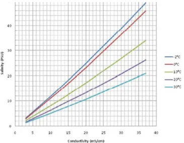
conductivity (ion content) of the pore fluid. An important source for ions is the amount of salt in the pore fluid, therefore the conductivity of the pore fluid depends strongly on its salinity. Fig.
5.19 shows the relationship between salinity and pore fluid conductivity for different temperature values. The relationship between the bulk resistivity of sediment, porosity and pore fluid resistivity may be described by the experimentally derived Archie’s Law, which holds for most sediments with little clay content:
rbulk = a f-m S-n rfluid
Where rbulk and rfluid are the resistivities of the seafloor and pore fluid respectively, F is the porosity, S denotes the pore fluid saturation, and a, m and n are constants, which range between 0.5-1.5 , 1.8-2.4 and ~2 respectively in marine sediments. Rocks containing large amounts of clay have a resistivity lower than predicted by Archie’s law due to conductive pathways along the surface of negatively charged clay particles.
Typical seawater resistivity varies between 0.3 to 0.5 Wm depending on seawater salinity and shallow marine sediments typical have a bulk resistivity of around 1 Wm. Fresh water resistivity ranges between 1 and 10 Wm, thus the bulk resistivity increases by a factor of 3 to 30 for fresh water saturated sediments.
Bulk electrical resistivity of marine sediments can be derived by a variety of methods, of which three (Magnetotellurics, CSEM and MMR) were used during OMAX. The difference between the methods arises from the geometry and frequency content of the electromagnetic source wave used and the geometry of the receiver. In magnetotellurics natural varying geomagnetic fields caused by currents in the ionosphere and worldwide lightning activity, give rise to electromagnetic source field. Since high frequency variations are damped by the conductive ocean above the measurement plane, the resolution in the upper kilometre is limited. However, bottom times of a few days or more allow the derivation of low frequency impedance values which allow for a depth of penetration of about 5 to 10 km. A shallow and higher resolution image of seafloor resistivities may be derived by controlled source electromagnetic measurements, which encompasses the use
Fig. 5.19 Pore fluid conductivity for different salinity values and temperatures.
of a transmitter to generate high frequency waves at the seafloor. Here we used a so called in line electric dipole-dipole systems, consisting of a horizontal electric dipole transmitter and inline dipole receivers. In addition to these more established methods, we also made a test measurement using the so called magnetometric resistance method (MMR). This method employs a vertical dipole as a source field and magnetic field receivers as receivers.
5.2.2 Magnetotellurics
5.2.2.1 Methodology
Natural varying magnetic field variations used in MT exhibit a plane wave characteristic.
Frequency dependent electrical impedance measurements (E(w)/B(w), where E(w) denotes the electric and B(w) the magnetic field as a function of frequency w) on the seafloor can in that case be shown to depend only on resistivity variations withing the ocean and underlying seafloor.
Impedance measurement can therefore be used to derive electrical resistivity models of the subsurface
In a homogenous half-space, the so-called skin depth d is a crude estimate of detection depth given by = 500 sqrt (r T) in meters, where T is the period in seconds and r is the bulk resistivity. Due to the shallow water depth we expect a high frequency limit of approximately 1 Hz in the data. The lower frequency is bounded by the length of time that the instruments measure on the seafloor and will be on the order of 10-4 Hz. We therefore expect to be able to derive a background resistivity model of the area down to approximately 100 km with a highest resolution of the upper layers of about 1 km. The model at greater depth might be limited due to the proximity of the coast, which deviates the induced current in the ocean layer around the resistive island and might cause a bias in the model, unless considered explicitly with 3D modelling.
5.2.2.2 Instrumentation
The GEOMAR OBEM (Fig. 5.20) is mounted on an instrument carrier which consists of a titanium frame on which syntactic foam elements are mounted to give the frame a positive buoyancy. For deployment, a magnetically neutral concrete anchor slab is attached to the frame
Fig. 5.20 GEOMAR OBEM lander.