2. MIS 11 Terminology

Matt O'Regan , Robert Poirier , Helen Coxall, Gary S. Dwyer, Henning Bauch , Ingalise G. Kindstedt^1,10, Martin Jakobsson⁶ , Rachel Marzen⁷ , and Emiliano Santin¹¹

1Florence Bascom Geoscience Center, U.S. Geological Survey, Reston, VA, USA,²Department of Earth and Planetary Sciences, Harvard University, Cambridge, MA, USA,³Department of Geosciences, Princeton University, Princeton, NJ, USA,⁴Department of Climate Geochemistry, Max‐Planck Institute for Chemistry, Mainz, Germany,⁵Earth and Environmental Science, Rensselaer Polytechnic Institute, Troy, NY, USA,⁶Department of Geological Sciences, Stockholm University, Stockholm, Sweden,⁷Lamont‐Doherty Earth Observatory, Columbia University, Palisades, NY, USA,

8Nicholas School of the Environment, Duke University, Durham, NC, USA,⁹GEOMAR Helmholtz‐Zentrum für Ozeanforschung Kiel, Kiel, Germany,¹⁰University of Maine Climate Change Institute, University of Maine, Orono, ME, USA,¹¹Atmospheric, Oceanic, and Earth Sciences, George Mason University, Fairfax, VA, USA

Abstract

Marine Isotope Stage 11 from ~424 to 374 ka experienced peak interglacial warmth and highest global sea level ~410–400 ka. MIS 11 has received extensive study on the causes of its long duration and warmer than Holocene climate, which is anomalous in the last half million years. However, a major geographic gap in MIS 11 proxy records exists in the Arctic Ocean where fragmentary evidence exists for a seasonally sea ice‐free summers and high sea‐surface temperatures (SST; ~8–10 °C near the Mendeleev Ridge). We investigated MIS 11 in the western and central Arctic Ocean using 12 piston cores and several shorter cores using proxies for surface productivity (microfossil density), bottom water temperature (magnesium/calcium ratios), the proportion of Arctic Ocean Deep Water versus Arctic Intermediate Water (key ostracode species), sea ice (epipelagic sea ice dwelling ostracode abundance), and SST (planktic foraminifers). We produced a new benthic foraminiferalδ¹⁸O curve, which signifies changes in global ice volume, Arctic Ocean bottom temperature, and perhaps local oceanographic changes. Results indicate that peak warmth occurred in the Amerasian Basin during the middle of MIS 11 roughly from 410 to 400 ka. SST were as high as 8–10 °C for peak interglacial warmth, and sea ice was absent in summers. Evidence also exists for abrupt suborbital events punctuating the MIS 12‐MIS 11‐MIS 10 interval. Thesefluctuations in productivity, bottom water temperature, and deep and intermediate water masses (Arctic Ocean Deep Water and Arctic Intermediate Water) may represent Heinrich‐like events possibly involving extensive ice shelves extending off Laurentide and Fennoscandian Ice Sheets bordering the Arctic.

1. Introduction

The climatic interval known as the Marine Isotope Stage 11 (MIS 11) was a long (~40,000–50,000 years), warm interglacial period with the warmest temperatures and highest global sea level between ~410 and 400 ka (kiloannum). MIS 11 climate has puzzled researchers for years because orbital insolation patterns and atmospheric CO₂concentrations were like those of the Holocene interglacial (Masson‐Delmotte et al., 2006), but many paleo‐records and climate models indicate higher global sea level and warmer climatic con- ditions (Past Interglacials Working Group of PAGES, 2016), especially at higher latitudes (de Vernal &

Hillaire‐Marcel, 2008).

MIS 11 sea level was probably 6 to 13 meters above present sea level (Dutton et al., 2015); however, higher (up to 20 m; Olson & Hearty, 2009) and lower (near present sea level; Bowen, 2010, Bauch & Erlenkeuser, 2003) global estimates and regional variability exist (Raymo & Mitrovica, 2012; see Rohling et al., 2009;

Elderfield et al., 2012; Spratt & Lisiecki, 2016). Nonetheless, on a global scale, sea level during MIS 11 is generally believed to have been higher than in both Holocene and last interglacial periods (MIS 5e, Eemian, ~6–9 m above present, Kopp et al., 2009). While SST were higher than Holocene in the Atlantic Ocean (Bauch et al., 2000) and lower in other regions (Milker et al., 2013), there is evidence they were rela- tively stable compared to the Holocene (Kandiano et al., 2017; Palumbo et al., 2019).

In addition to high global sea level and warm climatic conditions, the duration of MIS 11, by some estimates up to 40 kyr long (Berger & Loutre, 2002; McManus et al., 1999; Rohling et al., 2010), exceeds that of other

©2019. American Geophysical Union.

All Rights Reserved.

Special Section:

Special Collection to Honor the Career of Robert C.

Thunell

Key Points:

• The Arctic Ocean experienced warm sea‐surface temperatures and seasonally sea ice‐free conditions during interglacial Marine Isotope Stage 11

• Peak warmth and minimal sea ice occurred during the middle to late part of the interglacial followed by increased land ice and ice shelves

• Heinrich‐like events occurred in the Arctic during the MIS 12‐MIS 11 transition (Termination V) and during the MIS 11‐MIS 10 transition

Supporting Information:

•Supporting Information S1

•Data Set S1

Correspondence to:

T. M. Cronin, tcronin@usgs.gov

Citation:

Cronin, T. M., Keller, K. J., Farmer, J.

R., Schaller, M. F., O'Regan, M., Poirier, R., et al. (2019). Interglacial

paleoclimate in the Arctic.

Paleoceanography and Paleoclimatology,34

https://doi.org/10.1029/2019PA003708

Received 1 JUL 2019 Accepted 16 OCT 2019

Accepted article online 13 NOV 2019 , 1959–1979.

Published online 7 DEC 2019

Quaternary interglacials. For example, at Ocean Drilling Program (ODP) Site 646 south of Greenland, the dominant spruce (Picea) andfir (Abies) pollen signify an extended (nearly 50 kyr) MIS 11 interglacial with a“nearly ice‐free Greenland”and higher than present North Atlantic SST in the western subpolar North Atlantic (de Vernal & Hillaire‐Marcel, 2008). The latter, however, contrasts with the Nordic seas, where rather cold SST persisted during MIS 11 probably caused by a massive impact of MIS 12 deglaciation on sur- face stratification and winter sea ice formation (Kandiano et al., 2012, 2016; Thibodeau et al., 2018).

Moreover, the presence of ice‐rafted debris (IRD) across MIS 11 in the southwestern Nordic seas would argue for continual iceberg presence there and for an existing east Greenland Ice Sheet with glaciers reaching down to sea level.

Understanding high‐latitude cryospheric and climate variability during MIS 11 helps determine the sensitiv- ity of Greenland and Antarctic Ice Sheets to atmospheric CO2(Jouzel et al., 2007); the role of orbitally driven insolation (Rohling et al., 2010; Willeit et al., 2019; Yin & Berger, 2015); the phenomenon of Arctic Amplification, that is, amplified warming in Arctic regions due to sea ice loss and other processes, relative to global mean temperature (Cronin et al., 2017); and the potential for abrupt, millennial scale events during warm climate intervals (McManus et al., 1999). Importantly, MIS 11 is also relevant for understanding the evolution of climate during the Holocene interglacial, specifically for distinguishing natural climate variabil- ity from anthropogenic influence on climate (Palumbo et al., 2019; Ruddiman, 2007).

The current study examines the paleoceanography of the Arctic Ocean during MIS 11 using several proxies from sediment cores located mainly in the western and central Arctic Ocean (Figures 1 and 2, Table 1). Our main objective was tofill an important geographic gap in proxy records of MIS 11 climate that might aid in paleoclimate modeling of sea level and climate during past warm periods (Kleinen et al., 2014; Otto‐Bliesner et al., 2017; Raymo & Mitrovica, 2012). Specifically, we focus on the following questions: Did peak MIS 11 warmth occur in the Arctic Ocean early in the MIS 11 interglacial, as during the Holocene (MIS 1;

Kaufman et al., 2009, 2016; Briner et al., 2016) or during the middle or latter part of MIS 11 (Rodrigues et al., 2011)? What were sea ice conditions during MIS 11? Do SST and IRD records suggest abrupt suborbital events punctuating MIS 11 in the way that Heinrich events (HE) punctuated the last glacial period (MIS 4‐

MIS 2, from 60 to 18 ka; Bassis et al., 2017)? Can paleoceanography of the Arctic, specifically sea ice condi- tions and the strength of inflowing Atlantic Water, be linked to those in the Nordic seas and North Atlantic Ocean, the northward flowing North Atlantic Current (NAC), and Atlantic Meridional Overturning Circulation (AMOC) (Sévellec et al., 2017)?

2. MIS 11 Terminology

Before proceeding, the following conventions for terminology require clarification. Glacial Termination V (also called Termination 5) was the major deglaciation that occurred during the MIS 12‐MIS 11 transition and is used in the traditional sense defined by oxygen isotope records of foraminifera (Broecker & Van Donk, 1970) and other proxies. Some records show suborbital “Younger Dryas‐like” reversals during Termination V (Helmke et al., 2005; Kandiano et al., 2012) although there is no formal nomenclature for these. Regarding substage terminology for MIS 11, various authors use different terms and definitions due in part to the subjective nature of defining glacials and interglacials based on choices of alignment of a proxy record to orbital parameters such as precession (e.g., Masson‐Delmotte et al., 2006; Ruddiman, 2007). The entire period known as the MIS 11 interglacial is dated from ~424 to 374 ka in the deep‐sea benthic forami- niferalδ¹⁸O stack (Lisiecki & Raymo, 2005). Substages of MIS 11 are often referred to using letter (i.e., MIS 11c and 11b; Voelker et al., 2010; Palumbo et al., 2019) or number notation (MIS 11.3 for peak interglacial and subdivisions of 11.22 11.23, and 11.24; Rodrigues et al., 2011). We use the number notation to signify substages or stadial periods when Heinrich‐like events occurred during the MIS 11‐MIS 10 transition.

The term MIS 11c, used by Kandiano et al. (2007) to designate the interglacial climatic optimum, was later refined to MIS 11c sensu stricto dated from ~420 to 398 ka (Kandiano et al., 2012). In a comparison with the Holocene (MIS 1), Kandiano et al. (2012) also identified an early climatic optimum phase ~420–411 ka and a late phase ~411–398 ka during MIS 11c. Kandiano et al. (2016) also recognized peak interglacial conditions in the Nordic seas during MIS 11c sensu stricto from ~419 to 400 ka when the subpolar planktic foraminifera Turborotalita quinqueloba (Natland) co‐occurred with the polar species Neogloboquadrina pachyderma (Ehrenberg; formerly calledN. pachydermasinistral coiling(s); see Darling et al., 2017). In terms of IRD

flux, in the central and eastern Nordic seas, a warm peak comes late as indicated by a phase with no IRD, around 404–406 ka (Kandiano et al., 2016).

In a modeling study of MIS 11 sea level, Raymo and Mitrovica (2012) identified peak eustatic sea level from

~410 to 400 ka, roughly consistent with orbitally tuned marine isotope records and coral reef highstands. As we see below, terminological differences have paleoceanographic implications related to changes in SST, ice rafting, freshwaterflux, and other factors. For our study, we consider MIS 11 to be dated at ~424–374 ka, based on the Lisiecki and Raymo (2005) benthic foraminiferalδ¹⁸O stack, and we designate the peak MIS 11 interglacial as MIS 11.3 ~410–400 ka (see below).

Finally, Arctic Quaternary sediments contain a distinct stratigraphic zone dominated by the subpolar plank- tic foraminiferal taxon referred to asTurborotalia egelida(Cifelli & Smith).T. egelidamay be a morphotype of the speciesT. quinqueloba(Natland), and additional taxonomic and ecological work is needed to refine its usage (O'Regan et al., 2019). Nonetheless, what we call the“egelidazone”was recognized in early studies (Backman et al., 2004; Herman, 1974; Poore et al., 1993) and, more recently, shown to be widespread in the Amerasian Basin (Cronin et al., 2014; Polyak et al., 2013) and central Arctic (O'Regan et al., 2019).

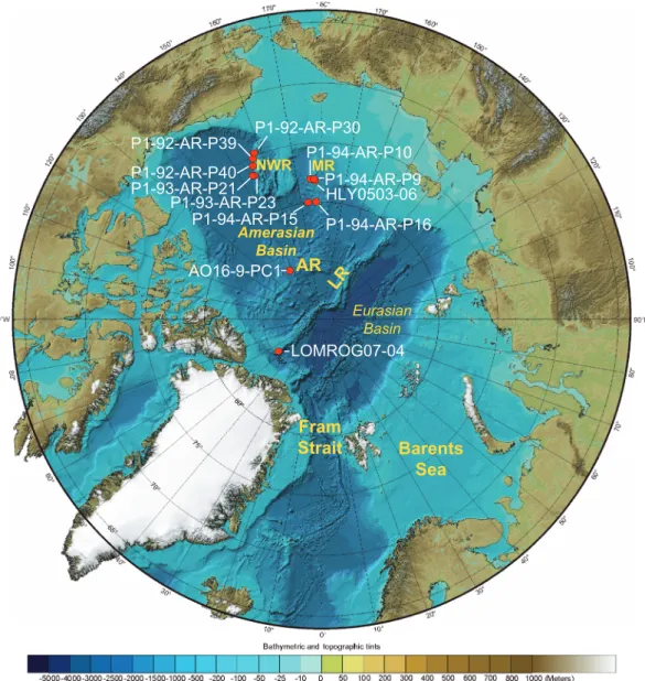
Figure 1.Map showing core locations (red dots) on the Northwind Ridge (NWR), Mendeleev Ridge (MR) and Lomonosov Ridge (LR) for the study of Marine Isotope Stage 11. Basemap from International Bathymetric Chart of the Arctic Ocean Version 3 (Jakobsson et al., 2012).

Theegelidazone is characterized by high abundance ofT. egelida(up to 90% total assemblage; Cronin et al., 2013), and often relatively small specimens (63–100 μm diameter), in contrast with most interglacial sediments dominated byNeogloboquadrina pachyderma(s)(Eynaud et al., 2009).

Typically, theegelidazone is between 12 and 63 cm thick depending on the core site sediment accumulation rate (Table 1, see section 5) and contains almost no coarse IRD, minimal sand‐sized material, and rare benthic foraminifers. Based on all available chronostratigraphic data for each core, we consider theegelida zone to represent the MIS 11 interglacial. In this zone,T. egelidaspecimens can be so abundant that they constitute the dominant element of the lithofacies. Occurrences of the better‐known subpolar planktonic foraminiferaT. quinquelobaare also observed in sediments dated to MIS 11 on the Lomonosov Ridge and also occur intermittently in post‐MIS 11 sediments (O'Regan et al., 2019). However, where recognized, the T. egelidazone is unique in its high abundance of this distinct enigmatic species/morphotype. Current understanding of Arctic Ocean planktonic foraminifera genetic diversity and biogeography (Darling et al., 2007, 2017) suggests thatT. egelidarepresents a subpolar migrant entering the Arctic Ocean from lower lati- tudes via the NAC either through the eastern Fram Strait or the Barents Sea. Migration from the Pacific Ocean via the Bering Strait cannot be totally excluded. For the current study, we consider theegelidazone an extremely useful biomarker for the MIS 11 interglacial in the Arctic Ocean (see Cronin et al., 2013;

Marzen et al., 2016).

3. Material and Methods

3.1. Sediment Cores and Ocean Setting

A total of 12 piston cores were studied; 6 yielded new benthic foraminifera stable isotope (δ¹⁸O_b) records (Figure 1, Table 1). In addition, two box cores and one trigger core were studied for benthic foraminiferal oxygen isotopes (δ¹⁸Ob) over the past ~40 ka. Cores were selected based on the preservation of faunal and geochemical proxies, core stratigraphy and chronology, and their locations in intermediate and deep water masses on the Northwind, Mendeleev, and Lomonosov Ridges (Schlitzer, 2016, Figure 2).

3.2. Chronology

There is a large literature on Quaternary orbital‐scale litho‐, bio‐, and chronostratigraphy in Arctic cores, including studies of planktic foraminifera (Poore et al., 1993), physical properties (color, grain size, and bulk density; O'Regan et al., 2008), oxygen isotopes (Polyak et al., 2004; Spielhagen et al., 2004), manganese layers (Jakobsson et al., 2000; Löwemark et al., 2014), elemental (calcium) concentrations (Wang et al., 2018), and microfossil density (a measure of biological productivity) (Marzen et al., 2016; Wollenburg et al., 2007), among others. Many studies use a cyclostratigraphic approach augmented by biostratigraphy to correlate and date sediments that are too old for radiocarbon dating. Biostratigraphic summaries of Arctic sediments using calcareous nannofossils, planktic and benthic foraminifera, and ostracodes which can be found in Backman et al. (2009), Stein et al. (2010), Polyak et al. (2013), Cronin et al. (2014), and references therein.

Additional age data come from amino acid racemization (Kaufman et al., 2008), strontium dating (Dipre Figure 2.Cross section of key Arctic Ocean locations and Arctic Ocean temperatures from World Ocean Atlas 2013 (https://www.nodc.noaa.gov/OC5/woa13/) plotted using Ocean Data View (ODV, Schlitzer, 2016).

et al., 2018) and Optically Stimulated Luminescence (Jakobsson et al., 2003). Magnetostratigraphy has also been attempted in Arctic sediments (reviewed in Xuan & Channell, 2010), but complications from self‐

reversals and anomalous excursions preclude its use as a chronological tool (Channell & Xuan, 2009).

Our approach was to use radiocarbon dating of the uppermost 10 to 30 cm of sediment from box and multi- cores (see Poirier et al., 2012), two key foraminiferal markers,Bolivina aculeata(a dominant species in MIS 5a, ~80 ka, summarized in Cronin et al., 2014) and the planktic speciesTurborotalita egelida(discussed above, ~400 ka; O'Regan et al., 2019), and cyclostratigraphy of calcareous microfossil density (benthic fora- minifera, ostracodes; Marzen et al., 2016). Due to highly varying sedimentation rates during glacial and interglacial cycles, we developed age‐depth models for each core using foraminiferal tiepoints and MIS boundaries identified from microfaunal density. These age models are given in Table 2 and illustrated in sup- porting information Figure S1. Theegelidazone in the Arctic Ocean, which we recognize in all of the cores discussed here, allowed us to align proxy records from different Arctic cores and correlate with records from the Nordic seas and North Atlantic.

3.3. Calcareous Microfossil Density and Productivity

The Arctic Productivity Index (API) is a composite“stack”constructed using benthic foraminifera and ostra- code density data (specimens per gram sediment per kiloannum) from 14 cores, each with its own age model.

The API stack was generated by aligning and binning microfossil records to a high‐resolution target record and generating an age model for the resulting stacked record by aligning it to the LR04 benthic foraminiferal oxygen isotope (δ¹⁸Ob) stack. This method was discussed in detail by Marzen et al. (2016). The group of cores covers 74.6 to 87.1°N latitude and water depths of 700 to 1900 m, thus sampling mainly AIW in the western and central Arctic. Benthic productivity can be measured using ostracode and benthic foraminiferal accu- mulation rates, which are closely linked to surface ocean productivity and foodflux (Marzen et al., 2016;

Wollenburg et al., 2004, 2007).

In the Marzen et al. (2016) study, API stacks were created for thefirst time, one for foraminifera, one for ostra- codes, and one for foraminifera and ostracodes combined. Because the aim of the initial study was to examine orbital‐scale variability, values were stacked in 2.5 cm bins for a target record with a sedimentation rate of

~0.5–2.5 cm/ka, limiting temporal resolution to events occurring on timescales longer than ~5 kyr. For the cur- rent study, we created higher resolution records by using smaller bins (i.e., 0.5, 1, 1.5 and 2 cm) for the stacked curves to examine suborbital patterns.

3.4. Benthic Foraminiferalδ¹⁸O

Five species of benthic foraminifera were used for stable isotopic analyses:Cassidulina teretis,Oridosalis tener, Cibicidoides wuellerstorfi, Pullenia bulloides, and Cassidulina reniforme. Foraminifera were brush‐ picked, and individual specimens were scored for visual preservation, ranging from 1 (transparent) to 4 (visual signs of alteration, including recrystallization and addition of authigenic mineral coatings). Of the five species, the three most abundant were used to develop the preliminary composite record presented here (C. teretis,O. tener, andC. wuellerstorfi). Discussion of benthic foraminiferal ecology and taxonomy is given in Wollenburg and Mackensen (1998), Osterman et al. (1999), Scott et al. (2008), Seidenstein et al. (2018), and Cronin et al. (2019).

A total of 326 oxygen isotope analyses were obtained, of which 317 analyses were on the 3 most common species; these were used to develop a compositeδ¹⁸Obstack back to 500 ka (see supporting information).

A minimum of ~30μg of foraminiferal calcite (~2–8 individual specimens) was used to perform each stable isotope analysis. Two hundredfifty‐six stable isotope analyses were conducted at Rensselaer Polytechnic Institute using an Isoprime dual inlet ratio mass spectrometer. Nineteenδ¹⁸O_bvalues onC. wuellerstorfi from trigger core HLY‐0205‐18tc were measured on a Thermo Delta V+ with Kiel IV device at the Lamont‐Doherty Earth Observatory (LDEO). Additional 46δ¹⁸Obvalues onC. wuellerstorfifrom box cores AOS94‐B16 and AOS94‐B17 were previously measured on a Finnigan MAT252 with Kiel device at Woods Hole Oceanographic Institution by Poore et al. (1999) and are included here. All measurements are reported in delta notation relative to Vienna Pee Dee Belemnite (VPDB) corrected to the NBS19 standard, with an average analytical precision (1σ) of ±0.05 (measurements from LDEO and Woods Hole Oceanographic Institution) and (2σ) of ±0.08 (measurements from Rensselaer Polytechnic Institute) onδ¹⁸Ob.

Table1 CoreDataforStudyofMIS11intheArctic CoreCoreabbreviationWaterDepth (m)LongitudeLatitudeºNGeographicLocationT.egelidadepth (cm)T.egelidaZone ThicknessMIS11‐Age/ DepthEq P1‐94‐AR‐P9P91035‐176.0478.133MendeleevRidge413‐42714y=5.4054 x‐1862.5 P1‐93‐AR‐P21P211470‐154.2176.86NorthwindRidge202‐23230y=2.6592 x‐183.51 P1‐92‐AR‐P30P30765‐158.0575.31NorthwindRidge585‐62540y=1.1562 x‐287.26 P1‐92‐AR‐P39P391470‐156.0375.84NorthwindRidge288‐33345y=0.8365 x+142.3 P1‐92‐AR‐P40P40700‐156.5576.26NorthwindRidge342‐40563y=0.7225 x+118.88 P1‐94‐AR‐P15P152726‐173.3280.2MendeleevRidge267‐30336y=1.4035x HLY0503‐6HLY‐6800‐176.2978.98615MendeleevRidge175‐20631Polyakeral2013 LOMROG04‐07LOMROG‐4811‐53.7786.7LomonosovRidge298‐31012Hansliketal.,2013 P1‐93‐AR‐P23P23951‐155.0776.95NorthwindRidge61‐8625Polyakeral2013 P1‐94‐AR‐PC16PC161568‐178.7280.333MendeleevRidge209‐23930y=1.4318+80 AO16‐9‐PC116‐9PC2212‐148.3385.9557AlphaRidge239‐25011Y=159 x‐10.8 P1‐94‐AR10P101673‐174.63378.15MendeleevRidge247‐26114y=1.8217 x‐67.318 *HLY0503‐18tcHLY18tc2654‐146.68388.45LomonosovRidgeNANA *Pl‐94AR‐B17B172217178.9781.27MendeleevRidgeNANA *Pl‐94AR‐B16B161533‐178.7180.34MendeleevRidgeNANA CorePrior AgeModel**Seaice‐Acetabulastomaδ18OMg/CaNADW‐KrithePlanktic SSTsOstracode DensityBenthicForam Density P1‐94‐AR‐P92134122 P1‐93‐AR‐P2123342 P1‐92‐AR‐P302134122 P1‐92‐AR‐P392134122 P1‐92‐AR‐P40213412 P1‐94‐AR‐P15333 HLY0503‐61,6141122 LOMROG04‐077322 P1‐93‐AR‐P231,2,6142,5 P1‐94‐AR‐PC161,23 AO16‐9‐PC133 P1‐94‐AR10332 *HLY0503‐18tc3x *Pl‐94AR‐B173x *Pl‐94AR‐B163x Sources,1Croninetal.,2013,2014,2Marzenetal.,2016,3Thispaper,4Croninetal.,2017,5DeNinnoetal.,2015,6Polyaketal.,2013,Dipreetal.,2018,7Hansliketal.,2013 *Boxandtriggercoresusedforlast40ka,noorbital‐scalesediment**SeeSupplementalFigureS1fordetailsofagemodelforeachcore.

Table2 AnchorPointsforOrbital‐ScaleTuningintheArctic AgeModel Segment1 CoreLengthT.egelidadepthT.egelida ThicknessMIS11 SedimentationrateDepth UpperDepth LowerEq#1Segment1 SedimentationRate P1‐94‐AR‐P9748.75413427141.016175y=0.7342 x+4.0591.4 P1‐93‐AR‐P21303.5202232300.571122y=0.9055 x+20.2111.1 P1‐92‐AR‐P30764585625401.52540y=0.6096 x+7.27971.6 P1‐92‐AR‐P39678288333450.81144y=0.7895 x+5.011.3 P1‐92‐AR‐P40530367411441.00166y=0.7674* x+3.3866 P1‐94‐AR‐P15761267303360.70285y=1.4035x HLY0503‐6236175206310.5 LOMROG04‐07514.5298310120.80.5117y=0.6095 x+20.8941.6 P1‐93‐AR‐P23560.756186250.218168y=1.0717 x+59.6161.1 P1‐94‐AR‐PC16650.5209239300.60224y=1.4318 x+80 AO16‐9‐PC1749239250110.6 P1‐94‐AR10596.5247261140.60169y=1.0717 x+59.616 AgeModel Segment2Segment3Segment4 CoreDepth UpperDepth LowerEq#2 Segment2 Sedimentation RateDepth UpperDepth LowerEq#3 Segment3 Sedimentation RateDepth UpperDepth LowerEq#4

Segment4 Sedimentation Rate P1‐94‐AR‐P9175309y=1.2638 x‐91.4530.8309404y=0.3885 x+179.97414423y=5.4054 x‐1862.5 P1‐93‐AR‐P21122230y=2.6592 x‐183.510.4230323.5y=1.1658 x+155.87 P1‐92‐AR‐P30540709.5y=1.1562 x‐287.260.9 P1‐92‐AR‐P39144232.8y=2.3169 x‐205.10.4233336.8y=0.8365 x+142.3 P1‐92‐AR‐P40166200interpolated200250y=2.1668 x‐239.98250425y=0.7225 x+118.88 P1‐94‐AR‐P15 HLY0503‐6 LOMROG04‐07117304.5y=1.6489 x‐102.10.6 P1‐93‐AR‐P23168266y=1.8217 x‐67.3180.5 P1‐94‐AR‐PC16 AO16‐9‐PC1 P1‐94‐AR10169313y=1.8217 x‐67.318 Note.SeeSupplementalFigureS1foranchorpointsandagedepthmodels.

Using published vital effect adjustments (Hoogakker et al., 2010; Kristjánsdóttir et al., 2007), and results from our own data, stable isotope values fromC. teretis(C. neoteretisto some authors; see Cronin et al., 2019) andO. tenerwere adjusted toC. wuellerstorfi, which calcifies its test in thermodynamic equilibrium with ambient seawater at low temperatures (Bemis et al., 1998). Adjusted isotope values were used to con- struct a composite record and scaled toUvigerinaby applying a constant adjustment of +0.64‰(Duplessy et al., 1984; Duplessy et al., 2002; Shackleton & Opdyke, 1973). Due to conflicting vital effect adjustments used in other studies ofC. teretis, we used paired analyses ofC. wuellerstorfiandC. teretisto evaluate avail- able adjustment values (Poole et al., 1994; Kristjánsdóttir et al., 2007; Groot et al., 2014; Chauhan et al., 2015). Our paired analyses exhibited a +0.45 ± 0.2‰meanδ¹⁸Oboffset forC. teretisfromC. wuellerstorfi, which is in general agreement with the vital effect adjustment (0.504‰) established by Kristjánsdóttir et al. (2007); see also Lubinski et al., 2001). Therefore, we applied a‐0.504‰adjustment toC. teretisstable isotope values, with the caveat that additional work is needed on benthic speciesδ¹⁸Ob offsets (Bauch et al., 2011; Bauch & Erlenkeuser, 2003).

3.5. Other Proxy Methods

In addition to the API productivity stack and new benthicδ¹⁸O_b records, this paper incorporates proxy records of bottom water temperature (BWT) based on ostracode magnesium/calcium (Mg/Ca) paleothermo- metry (Cronin et al., 2012, 2017; Farmer et al., 2012), sea ice cover based on abundances of an epipelagic ostracode species (Acetabulastoma arcticum; Cronin et al., 2010, 2013), and benthic ostracode taxa that are dominant in modern AIW and AODW (Cronin et al., 2014; Poirier et al., 2012). Results for each proxy record are discussed in section 5.

4. The MIS 11 Interglacial

4.1. Global Records of MIS 11

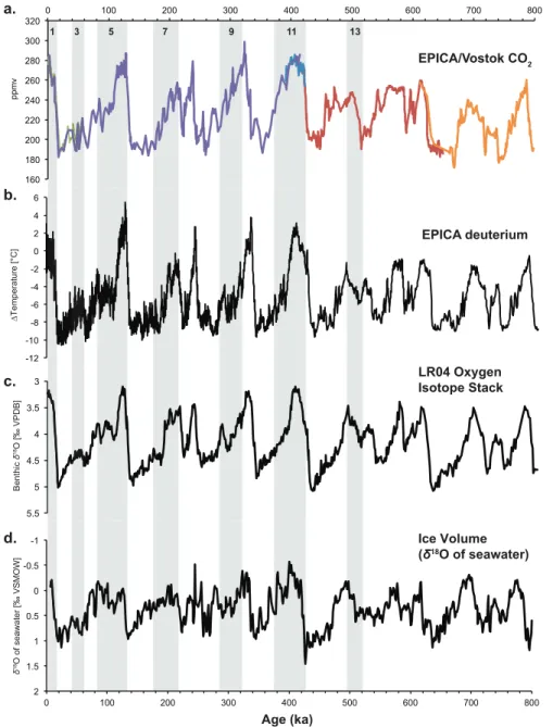
As background, Figure 3 presents“global”records of the last 800 ka to provide a context for examining the MIS 11 interglacial. Figure 3a is the combined record of atmospheric CO₂from several Antarctic ice cores showing (1) the ~40 ppmv increase in interglacial CO2levels from MIS 13 to MIS 11, during the Mid‐ Brunhes Event (MBE), roughly 450 to 350 ka, and (2) the sustained high preindustrial‐like interglacial CO2levels (at or just below 280 ppmv) during MIS 11 from 425 to 398 ka. These MIS 11 CO2concentrations, which use the age model of Yin and Berger (2015), remain relatively high for a longer duration compared to shorter periods of preindustrial‐like CO2during younger interglacials.

Figure 3b shows the Antarctic temperature curve derived from deuterium excess measurements from the EPICA Dome C ice core (Jouzel et al., 2007), which, although not strictly speaking a global temperature proxy, nonetheless exhibit a similar pattern to the CO₂curve and are considered a general indicator of Southern Hemisphere climate changes. The deuterium record during the MIS 11‐MIS 10 transition clearly exhibits large stadial‐likefluctuations in temperature during MIS 11.3, 11.2, and 11.1, which are smaller in amplitude but similar to Dansgaard‐Oeschger events of the last glacial cycle.

The marineδ¹⁸Obcurve (LR04; Lisiecki & Raymo, 2005; see also Spratt & Lisiecki, 2016), which is a compo- site“stack”constructed from 57 marine sediment core benthic foraminiferalδ¹⁸O records, is shown in Figure 3c. Oscillations inδ¹⁸Ob in LR04 represent the combined effects of global land ice volume and deep‐sea bottom temperaturefluctuations over orbital timescales. The curve shows the familiar sawtooth pattern of the“100‐kyr”climate cycles of the last 800 ka, a steady decrease inδ¹⁸O_b during the MIS 12‐ MIS 11 transition (Termination V), and minimal variation during interglacial MIS 11.

Theδ¹⁸Obcan be converted to theδ¹⁸Oseawaterwhen corrected for BWT changes using Mg/Ca paleothermo- metry. Elderfield et al. (2012) made such a reconstruction ODP Site 1123 from the Chatham Rise (Figure 3d).

Elderfield'sδ¹⁸O_seawaterrecord represents a global sea level/ice volume curve and, in contrast to the LR04 stack, exhibits large stadial‐like variability during the MIS 11‐MIS 10 transition. Rohling et al. (2009, 2010) also showed suborbital variability in sea level/ice volume during the MIS 12‐MIS 11 transition based onδ¹⁸Oseawaterconstructed from Red Sea planktic foraminiferalδ¹⁸O (see also Rohling et al., 2014). These types of suborbital events are also seen in the Arctic records discussed below.

4.2. Nordic Seas and North Atlantic Marine Records of MIS 12‐MIS 10

The warm, saline NAC, whichflows into the central Arctic Ocean proper through the eastern Fram Strait and Barents Sea, influences equator‐to‐pole heat transport and AMOC. The NAC submerges after entering the Arctic forming the subsurface Atlantic Layer (AL), which circulates within the central Arctic Ocean basin. The AL is a critical source of heat bounded above by the Polar Surface Water and below by AIW and Arctic Ocean Deep Water (AODW) (Rudels, 2015). Variability in the temperature and salinity of the NAC and the strength of the AMOC will impact the AL, as well as upper AIW, and is thus critical for corre- lating suborbital events in the two regions (Bauch, 2013).

Figure 3.Global paleoclimate records showing pattern during Marine Isotope Stage 11 compared to other interglacial periods. (a) Compilation of AntarcticpCO₂(atmosphere) records from EPICA Dome C, Taylor Dome, and Vostok ice cores (from Petit et al., 1999; Siegenthaler et al., 2005; Lüthi et al., 2008, and references therein; note that Bereiter et al.

(2015) corrected CO₂measurements from 800 to 600 ka but changes are minor and do not materially affect the CO₂curve for the MIS 11 interval). (b) Antarctic EPICA deuterium record from Jouzel et al. (2007) plotted as change in

temperature. (c) LR04 benthic foraminiferalδ¹⁸O isotope stack compiled from 57 cores (Lisiecki & Raymo, 2005).

(d)δ¹⁸O_seawater(in‰VSMOW) based on benthic foraminiferalδ¹⁸O_calcitefrom ODP site 1123 Chatham Rise from Elderfield et al. (2012).

Several high‐resolution paleoceanographic records from the North Atlantic‐Nordic seas region reveal high‐

amplitude changes in the NAC source water. McManus et al. (1999)first showed at ODP Site 980 in the sub- polar North Atlantic Ocean that significant suborbital variability over the last 500 ka occurred when ice sheets reached a critical size. This variability was later confirmed by Helmke and Bauch (2003), Kandiano and Bauch (2007), and Kandiano et al. (2016) for the Nordic seas and in midlatitudes of the northeast North Atlantic by Voelker et al. (2010), Rodrigues et al. (2011), Doherty and Thibodeau (2018), and Kandiano et al. (2017).

Figure 4 shows several of these proxy records for the period MIS 12 through MIS 10 (450 to 350 ka) going from north (top, panel 4a) to south (bottom, panel 4j). These records show that IRD typically increased dur- ing Heinrich‐like event excursions in both MIS 12‐MIS 11 and MIS 11‐MIS 10 transitions in the Nordic seas (core MD99‐2277) and the North Atlantic (cores M23414, U1313, and core U1308; Hodell et al., 2008).

Second, all curves are relativelyflat during peak MIS 11 interglacial 410 to 400 ka, reflecting a relatively stable climate with almost no IRD, high SST as derived from alkenones (MD03‐2669) andδ¹⁸O of planktic foraminifers (MD99‐2277, ODP 980, U1313), and high abundance ofN. pachyderma(M23414). All benthic δ¹⁸O records (ODP 980, M23414, and U1313), which are probably recording changes in either bottom tem- perature or strength of overturning circulation, show a similar glacial‐to‐interglacial pattern with a rapid

~1.8‰to 2‰decrease from MIS 12 to MIS 11 and a progressive increase during MIS 11 to MIS 10.

Taken together, these records show that suborbital variability linked to glacial processes and ocean circula- tion were fundamental features both during Termination V and the MIS 11‐10 transition in regions of the Nordic seas and North Atlantic. Transient suborbital cold events during Termination V were likely triggered by freshwater influx from melting ice, perhaps the Greenland Ice Sheet, and they affected surface, middepth, and deeper water layers as well as the AMOC (Kandiano et al., 2017). Similarly, during the transition into the MIS 10 glacial starting about 395 ka, there were multiple cool/warm cycles reflecting a weakening AMOC similar to those seen in HE during the MIS 5a‐MIS 3 interval (Voelker et al., 2010).

4.3. Prior Studies of Arctic Ocean Abrupt Climate Events

Several studies have identified glacio‐marine sedimentation and ice‐rafted events in the Arctic Ocean. For example, Darby et al. (2012) postulated 1,500‐year cycles in sea ice drift during the Holocene related to millennial‐scale events. Darby et al. (2002) interpreted layers containing iron oxides diagnostic of a North American provenance as times of ice sheet collapse and ice export from the Arctic and linked them to HE known from the North Atlantic Ocean during the last glacial going back to 34 ka. Ice‐rafted detrital sedi- ments known as“pink‐white”layers (mainly Paleozoic dolomite; Clark et al., 1980; Polyak et al., 2009;

Stein et al., 2010) are also widely recognized throughout much of the Arctic for the past ~150 ka and inter- preted as evidence for calving events from the Laurentide Ice Sheet. However, there has been no investiga- tion of sediment core records of ice sheet, ice shelf, and sea ice sensitivity during Termination V (MIS 12‐MIS 11), within MIS 11, or during the MIS 11‐MIS 10 interglacial‐to‐glacial transition despite their potential importance in high‐latitude abrupt climate transitions (McManus et al., 1999).

5. Results

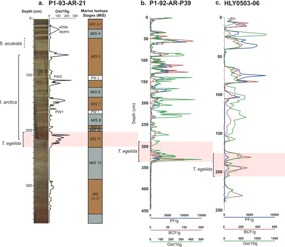
The stratigraphy of Arctic Quaternary sediments provides a necessary context for reconstructing paleoceano- graphic and glacial history. Marine sediments from Arctic submarine ridges are typically composed of alter- nating brown (interglacial) and gray/tan (glacial) sediments characterized by changes in density, magnetic susceptibility, manganese content, and calcareous microfossil abundance. Brown interglacial sediments typically have high microfossil density; in glacial intervals, microfossil density is usually lower, although this pattern varies from site to site. Figure 5a shows a photograph of a typical sediment core, the location of det- rital pink‐white layers, the abundance of microfossils, and key biostratigraphic events including the MIS 11 egelidazone. Figures 5b and 5c show three density curves of calcareous microfossil groups (planktic, benthic calcareous foraminifers, and ostracodes), as well as theegelidazone, for two other cores. This stratigraphy is recognized throughout most of the Arctic Ocean (Polyak et al., 2009; Poore et al., 1993; Stein et al., 2010 and references therein).

For context for the following discussion, Figure 6 shows the last 600 ka for six proxy records on orbital time- scales. Figure 7 shows suborbital variability in expanded curves for the 450–350 ka interval for the API, BWT derived from Krithe Mg/Ca, AODW (abundance of the genus Krithe) and benthic foraminiferal δ¹⁸Ob

records, as well as the SST reconstructions derived from planktic foraminifers identified by Kandiano in Cronin et al. (2013).

5.1. Arctic Productivity

Arctic productivity tends to be higher and more variable during interglacial periods than during glacial per- iods (Figure 6a). A notable exception is the period from MIS 9 through MIS 7, where Arctic productivity Figure 4.High‐resolution paleoceanographic records from the Nordic seas and the northeast Atlantic Ocean (going from north [top] to south [bottom]) showing suborbital variability during Marine Isotope Stages 12‐11‐10 (450 to 350 ka).

(a) Ice‐rafted debris (IRD) (grains >250μm per gram) and (b)δ¹⁸O ofNeogloboquadrina pachyderma(s) from core MD99‐ 2277 in the Norwegian Sea (Helmke et al., 2005; see also Kandiano et al., 2016); (c) benthic and (d) planktic

foraminiferalδ¹⁸O from ODP Site 980 in subpolar North Atlantic (McManus et al., 1999); (e) benthic foraminiferalδ¹⁸O and (f) percentNeogloboquadrina pachyderma(s) [red curve] and IRD [blue curve] from core M23414 in northeast Atlantic (North Atlantic Current; Kandiano & Bauch, 2007; Kandiano et al., 2012); (g) IRD, (h) benthic foraminiferalδ¹⁸O, and (i) planktic foraminiferalδ¹⁸O from IODP Site U1313 in the North Atlantic Current (Voelker et al., 2010); and (j) sea‐ surface temperature (SST) from MD03‐2669 off Portugal based on alkenones (Rodrigues et al., 2011). Peak interglacial MIS 11.3 and several stadial events are highlighted in vertical shaded regions.

displays peak values and high variability during MIS 8, a generally weak glacial period. The three productivity peaks during MIS 5 might represent MIS 5.1 (70 ka), MIS 5.3 (100 ka) and MIS 5.5 (125 ka).

In the period spanning MIS 12‐MIS 10 (Figure 7a), productivity increases steadily with the onset of MIS 11 and subsequently decreases in a gradual manner characterized by high variability during the transition into MIS 10. These patterns are interpreted as signifying suborbital stadial events (see below). Low API values during MIS 10 reflect the presence of thick sea ice and ice shelves limiting the penetration of sunlight and minimal surface productivity.

5.2. BWT

The BWT reconstruction in Figure 6b is derived from the Mg/Ca‐temperature calibration of the Arctic ostra- code (Krithe) (Farmer et al., 2012) applied to several cores covering the last 500 ka (Cronin et al., 2012, 2017).

In contrast to deep‐sea Mg/Ca records from outside the Arctic, which show deep glacial cooling, the inter- mediate depth Arctic warms during glacials and stadials due to submerging NAC inflow, forming the AL in the Arctic Ocean, below up to 1 km thick ice shelf cover (Jakobsson et al., 2016; Nilsson et al., 2017).

This deep water warming is interpreted to take place due to reduced fresh water influx during colder condi- tions, in turn causing the cold halocline to deepen and thereby driving the AL deeper (Jakobsson et al., 2016;

Nilsson et al., 2017). This can be seen during the last 50 kyr when BWT warming occurs during HE and the Younger Dryas (Cronin et al., 2012, Thornalley et al., 2015).

Figure 5.Typical stratigraphy and micropaleontology seen in three Arctic cores showing the location of several key marker beds modified from Cronin et al. (2014). (a) pink‐white (PW) layers 1 and 2 of detrital Paleozoic dolomite (Clark et al., 1980),Bulimina aculeata(late MIS 5),Bolivina arctica(MIS 5‐MIS 11), andTurborotalita egelida(MIS 11) plotted against Marine Isotope Stages, (b and c) density of planktic foraminifers (PF), benthic foraminifers (BF), and ostracodes (ost) in cores P1‐92‐AR‐P39 and HLY0503‐06, respectively.

During MIS 11.3, Arctic Ocean Mg/Ca values were relatively low varying within a ~1 mmol/mol range (Figure 6b). Mg/Ca ratios then gradually increase, punctuated by several cooling events corresponding to MIS 11.2 stadials. There are notable gaps in the composite record during the MIS 12‐MIS 10 and MIS 11‐ MIS 10 transitions, and further studies would be needed to establish this pattern with greater confidence.

In general, however, our records show that MIS 11 bottom temperatures from 700–1500 mwd were similar to temperatures at those depths in the modern Arctic Ocean. Figure 8 shows Mg/Ca ratios converted to °C from Figure 6.(a) Arctic Productivity Index constructed from benthic foraminiferal and ostracode density curves modified slightly into higher resolution binning from Marzen et al. (2016) using the stacking procedure in Lisiecki and Lisiecki (2002). Arctic productivity is an indicator of biological productivity in benthic ecosystems linked directly to near‐surface sea ice cover, algal primary productivity, and surface‐to‐seafloor foodflux. (b) Magnesium/calcium ratios of benthic ostracodes, a measure of BWT (Cronin et al., 2012; Farmer et al., 2012). Curve from Cronin et al. (2017). Note BWT increases during glacial and stadial periods due to the existence of thick ice shelves. (c) Relative frequency (percent abundance) of the genusKrithe, an indicator of cold oxygenated Arctic Ocean Deep Water and North Atlantic Deep Water.

(d) Relative frequency (percent abundance) of the genusPolycope, an indicator of warmer middepth Arctic Intermediate Water; (c and d) modified from Cronin et al. (2014). (e) Benthic foraminiferalδ¹⁸O_b(‰VPDB onUvigerinascale) uncorrected for BWT or ice volume (see supporting information). (f) Relative frequency (percent abundance) of the species Acetabulastoma arcticum, an indicator of perennial sea ice cover.

seven individual cores and compared to modern BWT values at each core site obtained from the World Ocean Atlas. It is clear that at all sites, MIS 11 BWT was roughly similar to modern BWT at the same depth and region of the Arctic Ocean. The most detailed record from core P40 (Northwind Ridge) shows a total range of BWT during peak MIS 11 and the transition into MIS 10 of about 1.5 °C. This range is lower than the BWT range in post‐MIS 11 glacial cycles (Figure 6b).

5.3. Arctic Ocean Deep and Intermediate Water

The presence of alternating periods of dominance by AODW and AIW, which may reflect shoaling and dee- pening of the AIW‐AODW boundary, is reflected in the relative abundances of two ostracode genera,Krithe Figure 7.Suborbital paleoceanography for the MIS 12, 11 and 10 interval from 450 to 350 ka, (a) Arctic Productivity Index (API) showing elevated values during peak MIS 11 interglacial conditions. (b) Magnesium/calcium (Mg/Ca) ratios showing low Mg/Ca ratios (lower bottom water temperatures, BWT) during peak MIS 11, and increasing BWT in the MIS 11‐MIS 10 transition due to greater AIW influence and the development of thick ice shelves. (c) Relative frequency (RF, percent abundance) of the genusKrithe, an indicator of cold oxygenated Arctic Ocean Deep Water and North Atlantic Deep Water, which reaches maximum RFs during several intervals during MIS 11. The decline in % for this genus reflects less AODW, more AIW. (d) Benthic foraminiferalδ¹⁸O showing lowest values during peak MIS 11 and increasing values during MIS 11‐MIS12 transition due to increasing global ice volume and/or increasing temperature. (e) Estimated sea‐ surface temperature (SST) based on quantitative planktic foraminiferal assemblage study by E. Kandiano, as described in Cronin et al. (2013). SIMMAX and Transfer Function Technique (TFT) are not ideally suited for Arctic assemblages and estimated temperatures are considered preliminary pending further study.

andPolycope, respectively. During the MBE, which is centered on MIS 11,Polycopefrequency increases from near zero at the MIS 12‐MIS 11 transition to nearly 60% of the total ostracode assemblage by the onset of MIS 10, reflecting an increase in bottom temperature, probably due to greater AIW influence, during this period (Figure 6d). In contrast, the relative frequency ofKrithepeaks early during MIS 11, reaching 60% of the total ostracode assemblage, and subsequently declines, nearing zero with the onset of MIS 10 (Figure 6c). Figure 7 shows an expanded view of the decline inKritheabundance throughout the latter part of MIS 11, which indicates a relative decrease in cold AODW, and a relative increase in warmer middepth AIW. The MBE faunal shift from Krithe‐ to Polycope‐dominated benthic ostracode assemblages is one of the most significant faunal turnovers in the Quaternary history of the Arctic (Cronin et al., 2014) and is similar to that seen in benthic foraminifera from the same regions (Polyak et al., 2013).

5.4. Benthic Foraminiferalδ¹⁸O

Figure 6e presents a new benthic foraminiferalδ¹⁸O curve, compiled from nine different cores taken on the Northwind and Mendeleev Ridges (Table 1, supporting information). There are several notable gaps in this record (MIS 6, 8, and 12), due to the problem that calcareous microfossils are often not present in Arctic Ocean cores during glacial intervals, but results nonetheless provide a useful preliminary Arctic benthic δ¹⁸O curve to complement existing global marine δ¹⁸O compilations (LR04 curve; Lisiecki & Raymo, 2005;fig 3).

Theδ¹⁸O record is notable in that it does not show the characteristic sawtooth pattern of the LR04 curve shown in Figure 3c. In particular, it lacks the abrupt deglacial decrease, followed by a more gradual increase, inδ¹⁸O values for each 100‐kyr glacial cycle. Instead, the record shows gradual changes inδ¹⁸O trends across glacial cycles, as well as evidence for suborbital variability. In addition, the total glacial to interglacial range ofδ¹⁸O is about 0.8‰to 1.0‰, much less than the 1.7‰to 1.8‰range in the open ocean. This pattern can likely be explained by the aforementioned influence of warmer BWT (deeper occurrence of AL) during gla- cial and stadial periods in the Arctic Ocean.

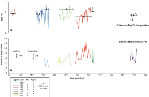
Figure 8.(a) Bottom water temperature estimates based on magnesium/calcium (Mg/Ca) ratios during Marine Isotope Stage 11 from seven Arctic Ocean cores plotted against core depth (cm). Different depths reflect different sedimentation rates. Horizontal bars (diamonds are mean value) give the modern (2005–2012) mean annual BWT from World Ocean Atlas 13 (https://www.nodc.noaa.gov/OC5/woa13/) at each particular core site's water depth from a 1° grid cell near the site. Mg/Ca‐temperature calibration 2.279 mmol/mol = 1 °C from Farmer et al. (2012); (b) Oxygen isotope values for benthic foraminifera from MIS 11 in six cores (‰VPDB). Both seawater temperature and global land ice volume influence δ¹⁸O. The scale to the left shows that an increase of 0.25‰would equal a 1 °C cooling and a 0.1‰change would equal about 10 m of sea level/ice volume change.

During MIS 11,δ¹⁸O oscillates between higher and lower values between substages 1, 2, and 3, reaching its lowest value (~3.4‰) at MIS 11.3 before the series of stadial events in the latter part of MIS 11 (Figure 7). The entire range of MIS 11δ¹⁸O values lies between 3.5‰and 4.5‰; for the most detailed record from P40 the range is 1.0‰(Figure 8). Figure 8 also shows that for the MIS 11δ¹⁸O records from six individual cores all display a decrease and subsequent increase inδ¹⁸O values throughout the interglacial. This pattern reflects combined changes in ice volume, temperature, and local hydrographic effects which contribute to the δ¹⁸O signal.

5.5. Paleo‐sea Ice

Acetabulastoma arcticumis an epipelagic, sub‐sea ice dwelling ostracode species used as an indicator for per- ennial sea ice. TheAcetabulastomarecord presented in Figure 6 contains data from nine sediment cores taken from the Mendeleev and Northwind Ridges in the western Arctic (HLY6, P10, P21, P23, P30, P39, P40, P9, P16) (Cronin et al., 2014, Figure 9; Cronin et al., 2017, Figure 3, new data from P10, P16). Figure S2a contains a new record from the Alpha Ridge region of the central Arctic (16‐9PC). Figure S2b shows a composite record of all sites incorporating the data from this core. Core AO16‐9PCfills a notable geographic gap in Arctic paleo‐sea ice reconstructions, as few sediment cores have been taken in the region of the Alpha Ridge in the central Arctic due to the presence of thick perennial sea ice. Finally, Figure 8 (upper panel) shows BWT based on ostracode Mg/Ca ratios from theegelidazone varied by over 1.0 °C (Cronin et al., 2017) and is approximately the same as modern bottom temperatures (black horizontal lines) near each site obtained from the World Ocean Atlas 13 (https://www.nodc.noaa.gov/OC5/woa13/).

In general, the low abundance ofAcetabulastomaduring MIS 11 is indicative of a seasonally ice‐free Arctic, including the Alpha Ridge region in the central Arctic. In addition, the MBE ~450–350 ka was not only a key transition in benthic faunas but also in the occurrence ofAcetabulastomaand, by inference, extended per- iods of perennial sea ice that was mostly absent prior to and during MIS 11 (Dipre et al., 2018; Polyak et al., 2013). The pattern of absence of summer sea ice during MIS 11 is in stark contrast to the common perennial sea ice at least during parts of younger interglacials (MIS 1, 3, 5, 7, and 9), which typically have high abundance ofAcetabulastoma. The absence or low abundance ofAcetabulastomaduring glacial periods is indicative of thick perennial sea ice or ice shelves limiting primary productivity, rather than a seasonally ice‐free Arctic.

5.6. SST

Planktic foraminiferal assemblages including commonT. egelidawere used to estimate MIS 11 SST in core HLY6 on the Mendeleev Ridge by E. Kandiano (in Cronin et al., 2013). The two methods included the SIMMAX method of Pflaumann et al. (2003) and a modified transfer function technique. Figure 7e shows estimated elevated summer SST between 440 and 435 ka, beginning at the onset of MIS 11, reaching from 6–7 °C to 8–10 °C during the peak MIS 11 interglacial. SST remained stable throughout the interglacial with the exception of a notable decline in temperature (1–2 °C) between 405 and 390 ka. These results must be considered preliminary as there exists no modern analog data set from surface sediments containingT. ege- lida. Nonetheless, as discussed above, theT. egelida‐dominated assemblage that is found throughout the Arctic during MIS 11 is in stark contrast to those in younger interglacial periods dominated by Neogloboquadrina pachyderma.

5.7. Discussion and Conclusions

Our results lead to a better understanding of MIS 11 in the Arctic on several fronts. Peak MIS 11 warmth in the Arctic Ocean seems to have occurred during the middle of MIS 11 roughly 410 to 400 ka if age models and correlations to extra‐Arctic records are correct. SST were as high as 8–10 °C at least for peak interglacial warmth, but additional SST proxy methods are needed. Sea ice conditions during MIS 11 were characterized by seasonally (summer) sea ice‐free conditions in many regions. These conclusions support the idea that Arctic Amplification is an inherent feature for at least some Quaternary interglacial periods.

There is also extensive evidence for abrupt suborbital events punctuating the MIS 12‐MIS 11‐MIS 10 interval.

Thesefluctuations in productivity, BWT, and deep and intermediate water masses (AODW and AIW) most likely represented Heinrich‐like events involving extensive ice shelves extending off Laurentide and Fennoscandian Ice Sheets bordering the Arctic. Such events, which punctuated the last glacial period (MIS 4‐MIS 2, 60 to 18 ka) in the Arctic (see above), are also consistent with evidence from submarine