Capacity Choices and Price Competition in Experimental Markets ¤
Vital Anderhub, Werner Güth,
Ulrich Kamecke, and Hans-Theo Normann Humboldt-Universität zu Berlin
Department of Economics Spandauer Str. 1
D-10178 Berlin Germany February 2001
Abstract
In the heterogeneous experimental oligopoly markets of this paper, sell- ers …rst choose capacities and then prices. In equilibrium, capacities should correspond to the Cournot prediction. In the experimental data, given ca- pacities, observed price setting behavior is in general consistent with the theory. Capacities converge above the Cournot level. Sellers rarely manage to cooperate.
¤We are grateful to Stephen Martin and Dorothea Kübler for helpful comments. Finan- cial support of the Deutsche Forschungsgemeinschaft (SFB373, Teilprojekt C5) is gratefully acknowleged.
1. Introduction
The Cournot (1838) model is among the most prominent models in economic the- ory. An often raised critique against this model is that, without special institutions like an auctioneer who sets the price, quantity competition lacks realism. Against this critique, an innovative justi…cation of Cournot competition was demonstrated by Kreps and Scheinkman (1983). They show that the Cournot solution may in- deed be justi…ed as the equilibrium outcome of a two-stage game in which sellers
…rst choose capacities and then, knowing the vector of capacities, sellers set prices.
Given the importance of the Kreps and Scheinkman model in justifying quantity competition, an empirical evaluation seems warranted. Two recent experimen- tal studies analyze capacity choices followed by price choices.1 More precisely, Davis (1999) analyzes posted–o¤er markets with three sellers and with advance production. In Muren’s (2000) paper, three sellers have to make a quantity pre- commitment before deciding about prices.
The experimental data support the Kreps and Scheinkman prediction only weakly.
Firstly, capacities are signi…cantly above the Cournot level in both studies. Sec- ondly, the experimental markets did not converge. The data indicate that sub- jects persistently made inconsistent choices, leading to instable markets. In Davis (1999), stable Cournot outcomes were not observed as play never converged with advance production. Similar results were obtained by Muren (2000): Markets were only stable with experienced participants who did the experiment twice.
Then the discrepancy between prediction and experimental outcome was some- what reduced, though not completely. Finally, price choices for a given capacity were neither in line with the theoretical prediction in both papers. This was also observed by Brown–Kruse et al. (1994). Their experiment was designed to test the prediction for the distribution of prices; there were no capacity choices. Price choices were inconsistent with the mixed strategy equilibrium distribution. Taken
1Field studies (Rosenbaum, 1989; Rees, 1993) of markets in which price competition is con- strained by capacities usually test for the collusive e¤ects of excess capacities (see Phlips, 1995, for a survey).
together, the problem with the evidence from the experimental studies is not that they simply reject the theoretical prediction, but rather the erratic choices of the subjects in general.
Why does the Kreps and Scheinkman theory fail in experimental markets? One possible explanation could be the analytical di¢culty of the intricate two-stage model. For example, Muren (2000, p. 154) mentions that even “in the experienced markets ... sellers did not seem to be entirely certain about the way the rationing mechanism worked”. Such uncertainties and misunderstandings may suggest that the Kreps and Scheinkman model is too demanding. Davis (1999, p. 72) has an alternative explanation. He conjectures that “the added complexity is not the primary explanation for the continued instability. ... The instability of the advance production environment is not due to the failure of the institutional framework to induce Cournot incentives, but rather to the instability of Cournot incentives themselves”.
In the light of these statements, it is interesting to recall that the Kreps and Scheinkman theory itself provoked criticism because of technical details. The main problem of their model is that no pure–strategy equilibrium in prices exists for generic ranges of capacity choices. The non–existence problem is caused by two discontinuities of the model. The …rst discontinuity results from the e¤ect of product homogeneity on the residual demand function. The second discontinu- ity is that, beyond the capacity constraint, production costs are in…nitely high.
This might lead to situations where the pro…t functions are not quasi concave.
Because of these features of the model, Kreps and Scheinkman have to make an assumption of how demand is rationed when prices di¤er and the low-price …rm cannot meet market demand. Kreps and Scheinkman apply the above mentioned e¢cient rationing. The e¢cient rationing rule implies that the low-price seller serves the buyers with the highest reservation values. This assumption is cru- cial for the results, in particular when analyzing endogenously chosen capacities.
Other rationing rules lead to di¤erent pricing behavior and thus to di¤erent en- dogenous capacities (see Davidson and Deneckere, 1986). In any event, the two discontinuities make the solution of the model technically very demanding.
Recent theoretical papers have modi…ed and generalized the Kreps and Scheinkman model, in particular with respect to these technical problems. Yin and Ng (1997) and Martin (1999) analyze capacity precommitment and price competition when products are di¤erentiated. Boccard and Wauthy (2000) and Güth and Güth (2000) analyze models with homogenous product competition, but capacities can be extended at a …nite extra cost. All these approaches con…rm the Kreps and Scheinkman result in the sense that the market equilibrium is à la Cournot.
In this experiment, we follow the line of these theoretical extensions. We will use a market model which assumes that goods are heterogenous and that capacities can be extended at a …nite extra cost. In this way, we avoid problems with the non–existence of pure–strategy equilibria and somewhat arbitrary rationing rules.
The capacity constraint is no longer an absolute upper limit on production, rather
…rms serve full market demand but at high costs. In this model, no matter how the distribution of capacities is, a (unique) pure–strategy in price is subgame perfect.
Moreover, the unique Nash equilibrium in prices and capacities is according to the Cournot prediction.2
We address the same problem as Davis (1999) and Muren (2000), namely the viability of the Cournot prediction in experimental markets with self–selected capacities, followed by price competition. We thought that it might be worth reducing the complexity of the game. Therefore, the major deviation from Davis (1999) and Muren (2000) is that we use the di¤erent market model just mentioned.
A second di¤erence in the experimental design is that capacity is …xed for several periods in our experiment. This allows subjects to learn optimal pricing strategies within each capacity constrained subgame. Thirdly, we start the experiment with exogenously …xed capacities. Again, the idea is that subjects should …rst get an idea of how to choose prices. Our conjecture is that in the simpli…ed environment the data might give a clearer picture about the Cournot-type results in Bertrand–
Edgeworth markets.
2Similar models were proposed by Güth (1995) and Maggi (1996). Güth (1995) discusses how to view homogeneity as a limiting case of heterogenous products. Maggi (1996) shows how the equilibrium outcome ranges from Bertrand to Cournot as capacity constraints become more important. For a very comprehensive analysis, see Martin (2000).
Our results are as follows. In contrast to Davis (1999) and Muren (2000), we found that price choices are in general consistent with the subgame perfect prediction, and that capacity choices are stable. However, capacity choices were often above the Cournot prediction. While we are able to rationalize the capacity-setting behavior, it is remarkable that hardly any cooperation occurs in our duopoly markets.
In Section 2 we introduce the market environment and derive the equilibrium. Our experimental design is described in Section 3. Section 4 discusses the experimental results. We conclude in Section 5.
2. Market model
Our experiment assumes a heterogeneous oligopoly market with n sellers whose demand functions are given by
xi(p) =®¡¯pi+°
0
@X
j6=i
pj
n¡1 ¡pi
1
A for i= 1; :::; n; (2.1) provided that all quantities are positive. Here p= (p1; :::; pn) denotes the vector of individual sales pricespj andxi(p)is selleri’s demand level as depending onp.
The positive parameters ® and¯ describe how demand depends on prices when all prices are equal, i.e. when pi =P
j6=i pj=(n¡1) for i = 1; :::; n. The positive parameter ° measures the degree of heterogeneity on the market. By ° ! 0; we could approach the situation where all n sellers are essentially monopolists, by
° ! 1a homogeneous market since small deviations from the average price would induce dramatic spill–overs of demand (what would rule out prices di¤erences).
Production requires investments in capacities x. We assume that capacity costs Ki(xi) =cxi; for i= 1; :::; n; (2.2) are linear in selleri’s capacityxi:Production costsCi(xi; xi)are (piecewise) linear Ci(xi; xi) =d maxf0; xi¡xig; for i= 1; :::; n: (2.3)
According to equation (2.3) the capacity xi is no rigorous upper bound for seller i’s sales levelxi. A capacityxi just represents a production target which does not preclude larger sales in the sense ofxi > xi, but only imposes positive extra costs d(xi¡xi); d > c; for positive excess demandsxi¡xi.
Due to market clearing, i.e.,
xi =xi(p) for i= 1; :::; n; (2.4) the actual sales level xi is determined by the vector pof chosen sales prices. The pro…ts per period resulting from these choices are
¦i(p; x) =pixi(p)¡Ki(xi)¡Ci(xi(p); xi); for i= 1; :::; n; (2.5) where x denotes the vector(x1; :::; xn) of individual capacities.
Firms play a two-stage game. They …rst choose capacities and then, knowing the vector of capacity choices, they choose their prices. In order to derive equilibrium behavior, consider the last stage …rst. Given the capacities x; there are three possible segments of the price reaction functions: One for the case of idle capacity, one where capacity is fully utilized, and one when there is excess demand (see Appendix A). If all …rms’ demand is equal to capacity, we can express price reaction functions solely in terms of capacities.3 We get
p¤i (x) =
(®¡xi) [¯(n¡1) +°] +° P
j6=i(®¡xj)
¯[¯(n¡1) +n°] (2.6)
as subgame perfect prices.
Then consider the …rst stage. We state three solutions of this model as benchmarks for the experiment (see Appendix A for the derivation). Consider …rst the joint- pro…t maximizing solution as a benchmark. We get
xci = ®¡¯c
2 for i= 1; :::; n; (2.7)
3Though capacity choices up to 200 were allowed by design, in the experiment, all capacity choices were in the range where demand should equal capacity. That is, subgame perfect prices would have always yielded production up to capacity. Collusive pricing also almost always implies production up to capacity. The reason is that leaving idle capacities maximizes the joint pro…ts only if capacities are very large. As such cases are very rare in our experimental data, we refrain from deriving the solution for collusive prices.
as the e¢cient and collusive capacity choices xci of all sellers, and pci = ®+¯c
2¯ fori= 1; :::; n; (2.8) as optimal prices.
The second theoretical benchmark is the Cournot-Nash solution in which the play- ers rationally recognize the in‡uence of their capacity choice on the competitors’
pricing behavior. The solution of the corresponding two-stage game is readily computed:
xni = [¯(n¡1) +n°] (®¡¯c)
2 (n¡1)¯+ (n+ 1)° for i= 1; :::; n: (2.9) Since equilibrium capacities are symmetric, prices are simply
pni = ®¡xni
¯ for i= 1; :::; n: (2.10) in equilibrium.
The third theoretical benchmark is a competitive solution in which the players ignore the oligopolistic price mechanism. Of course, price setting strategies are not compatible with the standard notion of a competitive allocation, but we can easily replace this by a scenario of monopolistic competition in which the players take the prices of the competitors as given and maximize the resulting pro…t function.
Note that in this case …rms play a one-shot game. As the solution, we get xwi = [¯+°] (®¡¯c)
2¯+° ; i= 1; :::; n; (2.11) and
pwi = ®+c(¯+°)
2¯+° : (2.12)
3. Experimental setup
In order to make the market as simple as possible, we decided to employ n = 2
…rms in the market. The other parameters were as follows. The parameters
®= 120, ¯ = 1and° = 2describe the demand functions such that (2.1) becomes xi(p) = 120¡pi+ 2 (p¡i¡pi) for i= 1;2; (3.1) given thatxi(p)>0; i= 1;2:If one …rm sets a high price such thatxi(p)<0;we made sure that the demand function for the remaining “active” …rm is adjusted.4
4One getsxi<0ifpi >(120 + 2pj)=3. Hence, ifxi <0, we setxi = 0, pi= (120 + 2pj)=3 and thereforexj= 200¡5=3pj in the computer program of the experiment.
Cost parameters were c= 40 for the capacity costs andd= 80for the production costs of every unit exceeding the capacity. Equation (2.6) becomes
p¤i(x) = 600¡3xi¡2x¡i
5 ; i= 1;2:
Further, we introduced a …xed cost of 600 in order to get a relatively larger and reasonable di¤erence between cooperative and non-cooperative pro…ts.
With these parameters, the symmetric collusive solution requires
xci = 40and pci = 80 for i= 1;2: (3.2) The non-cooperative Nash equilibrium implies
xni = 50and pni = 70 for i= 1;2: (3.3) Finally, the competitive benchmark is
xwi = 60 and pwi = 60 for i= 1;2: (3.4) Pro…ts resulting from these capacities and prices are1000 at the symmetric collu- sive solution, 900 at the non-cooperative equilibrium and 600 at the competitive solution.
The sellers interact repeatedly on this market in periodst = 1;2; :::;60;i.e. within a given and known …nite time horizon. Our setup also allows for cooperative outcomes to occur. There is ample evidence (Selten and Stöcker, 1986) of stable cooperation (except for a rather short end phase) even in the case of a known
…nite horizon, excluding so-called Folk Theorems.
Capacity was to be chosen every tenth period while the price was to be set in every period. A change in restructuring is seen as a major restructuring of the
…rm whereas prices can be more easily and frequently adjusted. In order to give participants an occasion to learn about the market, capacities are …rst exogenously given from t = 1 to 10 and anew from t = 11 to 20 respectively.5 The decision process assuming that all former choices are commonly known is as follows.
5In a pilot session, the design of the experiment was without such initial exogenous capacities.
It turned out that such a setup was too complicated. Subjects incurred substantial losses before converging to reasonable capacities so that they only broke even after 60 periods.
Stage 1: (in t= 21;31;41;51): Sellersi= 1;2 choose their capacitiesxi. Stage 2: (in t= 1;2; :::;60): Sellersi= 1;2 choose their sales prices pi,
The initial capacity vectors x= (x1; x2) for t= 1and t= 11 were x=
( (50;40) for t= 1; :::;10;
(45;65) for t= 11; :::;20. (3.5) The corresponding equilibrium price vectors p¤ = (p¤1; p¤2)are
p¤ =
( (74;76) for t= 1; :::;10;
(67;63) for t= 11; :::;20. (3.6)
Information was given to subjects in the following way. The cost parameters (40 for each capacity unit, and 80for each unit in excess of capacity), the number of
…rms (two), the number of periods (60), and the exchange rate of experimental earnings into real currency (see below) were explicitly mentioned in the instruc- tions (see Appendix B). Experiments were computerized.6 This enabled us to give more information on the computer screen. After each period, subjects learned the price choice of the rival …rm and the resulting pro…t for their own …rm. Similarly, they learned the choice of the rival …rm whenever capacities were chosen.
Moreover, subjects had access to a “pro…t calculator”. When considering their decisions, subjects could enter trial prices and capacities (numbers between 0 and 200 with two decimal points) in this calculator. The pro…t calculator gave a subject the sales and pro…ts of his or her own …rm which would occur with these decisions. Once actual capacity choices were made, they remained …xed in the pro…t calculator and subjects could only experiment with prices. Subjects could experiment with the pro…t calculator as intensively as they wished. With the device of the pro…t calculator, the demand conditions could quickly be learned.
Note that a pro…t calculator gives qualitatively the same information as a pro…t table. Such tables are often provided in market experiments of this kind (e.g.
Holt, 1985). They allow, however, only for a small and discrete action space. The
6We used the software “z-Tree” (Fischbacher, 1999).
pro…t calculator allows for many actions. As we had two decimal points for the capacity and price decisions, continuous actions were approximated. This has the advantage that multiple Nash equilibria due to the discretization of the action space (see Holt, 1985) can be avoided. An alternative design would have been to provide the functional form of the demand function to subjects (Davis, 1999;
Muren, 2000). However, since our design with product di¤erentiation requires more complicated functional forms, this does not seem to be practible. Compared to the provision of functional forms, the pro…t calculator might help to avoid a bias due to limited computational capabilities of subjects. Generally, it seems possible that the use of a pro…t calculator reduces the “noise” in the data that results from subjects making random noises.
The experiments were conducted in the computer lab of the Humboldt University.
We conducted three sessions, each consisting of six duopoly pairs. That makes a total of 36 subjects which were recruited via telephone and email from a list of participants of previous experiments. Each subject participated only once and no subject had participated an experiment similar to ours before. Subjects were randomly allocated to separated cubicles in the lab. They were not able to infer with whom they were interacting.
Sessions lasted between one hour and 45 minutes and two hours and 15 minutes.
For 1,000 “points” earned in the experiment, DM 1 was paid. An initial capital of 15;000 points was given since subjects could have made losses, particularly so in the beginning. Average earnings were DM50:99(which is roughly $27).
4. Results
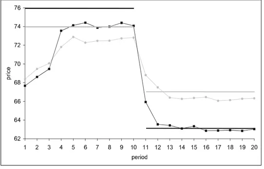
We start by reporting the results for pricing behavior. As mentioned, in periods t = 1; :::;20 capacities were exogenously …xed. In Figure 1 we have graphically illustrated the average price choices for the …rst 20 rounds (the solid lines indi- cating subgame perfect prices (74;76) and(67;63) respectively). Prices are often
below the predicted level, however, this deviation is rather small. Prices move to- wards the equilibrium prices. For the …rst set of capacities prices are, after some time of coordination, quite close to the prediction, and very close for the second exogenously given capacity vector.
Figure 1: Average price choices for predetermined capacities in t= 1; :::;20
How is pricing behavior when capacities are self-selected in later periods? In Table 1, we report the percentages of “hits”, that is, the relative frequency of subgame perfect price choices. We distinguish exact hits and price choices which were within a 5%range of the subgame perfect prices. We report these results for the entire data set, separately for all thirds (periods t = 1 to20; 21 to 40, and 41 to 60), and for the second halves of the ten-period interval with the same capacities (periods t = 6 to 10;16 to 20; :::;56 to 60:). The hypothesis behind this is that subjects make more accurate price choices over time. We also reports hits when capacity choices were symmetric. Here, the hypothesis was that subgame perfect prices are more easily found with equal capacities. Note that, for all observations, subgame perfect prices were such that demand would have equalled capacity, that is (2.6) was the appropriate price reaction function.
exact §5%
all observations (#2160) 33:47 85:83 t = 1; :::;20 (#720) 28:75 77:63 t = 21; :::;40 (#720) 36:81 86:53 t = 41; :::;60 (#720) 34:86 93:33 t = 6to10;16to 20; :::;56to60 (#1080) 35:37 91:02 symmetric capacities (#200) 72:00 99:50 Table 1: Relative frequency of subgame perfect price choices
In approximately one third of the cases, subjects played exactly the subgame per- fect prices (recall that there were two decimal points). Almost all choices were roughly equal to the subgame perfect prices. Looking at the tables in Appendix C, it is remarkable how close pricesp¤i and actual average prices were. It appears that participants understood the price implications of capacity vectors well. From Table 1, the frequency of hits in later periods within a ten-period subgame in- creases. It also appears that§5% hits increase over the course of the experiment.
Moreover, symmetric capacities seem to facilitate hits.
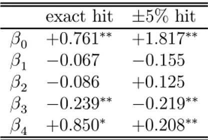
In order to test for statistic signi…cance of these e¤ects, we ran the simple regres- sion
h=¯0+¯1f irst+¯2last+¯3early+¯4symm;
where we take into account that observations are independent across sessions but not neccesarily within sessions.7 The number of “hits” (h; two at most) was the variable to be explained. The variable f irst was equal to one if t <21 and zero otherwise; similarly lastwas equal to one ift2(40;60]and zero otherwise; early was equal to one in periods t = 1 to 5, 11 to 15,..., 51 to 55 and zero otherwise;
symm was equal to one if capacity choices were symmetric. (see Table 2).
All coe¢cients have the expected sign, exceptlastfor exact hits. Subgame perfect prices are signi…cantly more likely when capacities are symmetric. The variables f irstandlastare not signi…cant, whileearly is. We interpret this as a con…rma- tion of our design (few capacity choices, several price choices within subgames).
There is learning going on within the ten period subgames, but prices do not become more accurate in the later periods of the experiment.
7We used thecluster option for linear regressions of the STATA package. See STATA Corp.
(1999, vol. 3, pp.156-158).
exact hit §5% hit
¯0 +0:761¤¤ +1:817¤¤
¯1 ¡0:067 ¡0:155
¯2 ¡0:086 +0:125
¯3 ¡0:239¤¤ ¡0:219¤¤
¯4 +0:850¤ +0:208¤¤
Table 2: Regression results for hit rates. Superscripts ¤¤(¤)indicate signi…cance at the 1(5)% level.
We summarize the results of the price setting stage as follows:
Observation 1: Participants quickly learn to rely on equilibrium prices p¤i satisfying xi(p¤) =xi for i= 1;2.
We now turn to the results of the capacity choices. In the tables in Appendix C, we list the four capacity vectors for all18markets. Since capacity choices are likely to depend on individual paths, we …rst report industry capacities, x1;2 =x1+x2; in Table 3. Recall that the predictions were 80 for the collusive market, 100 for the Cournot market and 120 for the competitive market.
x1;2 ¾(x1;2) t= 21; :::;30 114.2 18.6 t= 31; :::;40 110.0 16.1 t= 41; :::;50 109.9 14.7 t= 51; :::;60 109.5 14.9 Table 3: Average industry capacity
Out of 72 observations for industry capacity (see Appendix C), none was smaller than 80, 16 were smaller than 100, 37 were between 100 and 120, and 19 were larger than 120 with 153 being the maximum. Average industry capacity is110:93 which is above the Cournot-Nash equilibrium value and below the monopolistic
competition solution. The95%con…dence interval for industry capacity (again ac- counting for possible dependence of observations within groups) is[103:89;117:97]
around the observed mean. Therefore, we have to reject the hypothesis that ca- pacity choices coincide with the Cournot prediction, and we also have to reject the hypothesis that capacity choices are in line with monopolistic competition.
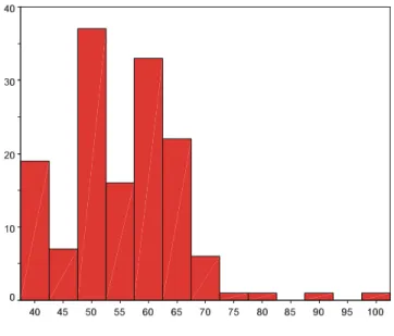
Figure 2: Histogram of the individual capacities
A look at the histogram of individual capacity choices in Figure 2 gives further insights. The Cournot equilibrium choice (50) is contained in the bracket which occurred most often. Ignoring the (somewhat arbitrary) brackets in Figure 2, we
…nd that 50 is also the mode of all capacity choices. The monopolistic competition solution (60) is the second most frequent choice while the intermediate value (55) is chosen less often then the collusive capacity.8 While there is some dispersion in capacity choices, these choices are relatively constant for individual industries (see Appendix C). Moreover, average capacity choices are, except for a slight (and insigni…cant) negative trend, stable over time.
Stable behavior which is more competitive than the Cournot solution was also found in Huck, Normann, an Oechssler (1999). In their quantity-setting homogen- ous-goods Cournot experiment, depending on the information revealed to subjects,
8The benchmark capacitiesxc1;2; xn1;2 andxw1;2 were chosen simultaneously by both …rms in 2;4;and1of the 72possible cases, respectively. Surprisingly, all price choices in all periods are optimal for these capacities in the sense thatxi(p) =xi(p); i= 1;2.
play converged close to the competitive equilibrium.9 And even when structural information was granted as in our study, the results were quite competitive. These results were con…rmed in experimental markets with quantity-setting …rms and di¤erentiated goods by Huck, Normann, an Oechssler (2000). However, in Huck, Normann, and Oechssler (1999, 2000), there were four …rms and, in Davis (1999) and Muren (2000), there were three …rms. Since we used duopoly markets, our results are surprising. In most standard Cournot duopoly experiments in which subjects are matched in …xed pairs, there is at least some cooperation and there are rarely choices beyond the Cournot level.10 We conclude from this that repeated interaction over a long but …nite horizon is no reliable reason for cooperating.
Observation 2: (i) Capacity choices are at a level above the Cournot prediction and below the competitive prediction. (ii) Despite the relatively long horizon, there is hardly any cooperation.
Since we have concentrated on n = 2 …rms, our test seems to provide the most favorable conditions for cooperation (since cooperation on larger markets is more doubtful, see Selten, 1972, for a rigorous distinction of small, i.e. cooperative markets with few sellers). Thus game types inviting cooperation seem to be: not framed as markets11, and relying on one-stage base games (or binary games).
It seems interesting to explore which of these aspects is (more) reasonable for inducing cooperative outcomes, but this is beyond the scope of this study. It seems that the strong cooperative results for …nitely repeated prisoners’ dilemma and public good provision games are special results for certain game types which are cognitively perceived as cooperative exercises.
Another reason for more competitive results is that our design relies on quite realistic assumptions concerning the pro…tability of cooperation. Whereas, in
9For our market model this would require both,°! 1andn! 1;and thusxi!80and pi!40:
10Concerning this issue, see e.g. Dufwenberg and Gneezy (2000), or Keser (2000). Selten et al. (1997) show that, in tournaments, there is a particularly strong motivation to establish collusion.
11Experiments framed as markets seem to induce more competitive behavior. See Ho¤man et al. (1994).
our experiment, cooperation leads to moderate increases in pro…ts, mutual co- operation in most base games (of …nitely repeated games with …xed matching) yields much larger, sometimes outrageous increases in pro…ts (see, for example, the repeated prisoners’ dilemma experiment of Cooper et al., 1996; or repeated interaction in trust games of Berg et al., 1995). It is quite possible that the usually claimed cooperation in …nitely repeated games is mainly due to the dominance12 of striving for e¢ciency when cooperation is highly pro…table. This may surprise naive protagonists of cooperative behavior or e¢ciency. From an antitrust per- spective, however, the result is most welcome since there might be competitive results even in narrow markets. It also allows to maintain the duopoly market as a standard case for illustrating the e¤ects of competition.
5. Conclusion
In this experiment, we tested for the viability of the Cournot prediction in duopoly markets with capacity and price competition. We used a simpli…ed environment which allowed subjects su¢cient time for learning of frequently adjusted choices (prices) and rarely adjusted choices (capacities). In contrast to other experiments (Davis, 1999; Muren, 2000), we found subgame perfect price choices and stable capacity choices. Individual capacities converge at a level below the competitive prediction and above the Cournot prediction. That is, capacity choices were more competitive than pure non–cooperative behavior suggests. It is surprising that no cooperation occurs in our duopoly markets with the same …rms interacting for 60 market periods.
12When one views decision making as the result of competing behavioral forces, it makes sense to assume that one can in‡uence behavior by changing the relative strength of one motivation, e.g. by weakening the gains from cooperation.
Appendix
A. Derivation of the benchmark solutions
We …rst derive subgame perfect prices given the installed capacities. The reaction function of each …rm has three di¤erent segments.
² Up to capacity, …rmi can produce at zero marginal cost. That is, if xi < xi we get
@¦i(p; x)
@pi
=®¡2(¯+°)pi+°
P
j6=ipj
n¡1 = 0; (A.1)
and therefore
p¤i = ®+°
P
j6=ipj
n¡1
2(¯+°) : (A.2)
The …rst part of the reaction function is relevant if it is optimal to hold idle capacity. In that case, …rmichooses its prices such that marginal revenue is zero.
² The second segment of the reaction function is relevant if marginal revenue is between zero and d. Here, …rm ichooses pi such thatxi =xi:
®¡(¯+°)pi+°
P
j6=ipj
n¡1 =xi; (A.3)
that is,
p¤i = ®+°
P
j6=ipj
n¡1 ¡xi
¯+° : (A.4)
In this segment, capacity is fully utilized. If reaction functions of all …rms intersect in this segment, we can use ¯Pnj=1p¤j = Pnj=1(®¡xj) to express p¤i in terms of capacities only:
p¤i (x) =
(®¡xi) [¯(n¡1) +°] +° P
j6=i (®¡xj)
¯[¯(n¡1) +n°] : (A.5)
² In the third segment, …rm i produces more than its capacity, at the extra cost d:
@¦i(p; x)
@pi =®¡2(¯+°)pi+°
P
j6=ipj
n¡1 + (¯+°)d= 0; (A.6)
and so
p¤i = ®+°
P
j6=ipj
n¡1 + (¯+°)d
2(¯+°) : (A.7)
Here, marginal revenue is larger thandand therefore it is rational to produce the excess demand units.
The slope of reaction function di¤ers in the three segments: @p¤i=@pj is larger in the second segment. It is easy to verify that 0 < @p¤i=@pj < 1=(n¡1) in any segment, therefore a unique vector of prices exists for any combination of capacities.
Our …rst benchmark is the joint–pro…t maximum. Perfect collusion requires e¢- ciency in the form of xi(p) = xi for all sellers i = 1; :::; n; and symmetry in the form of xi =xj for alli; j = 1; :::; n. We can therefore set xj =xi for allj 6=i in equation (A.5) so that
p¤i (xi) = [¯(n¡1) +n°] (®¡xi)
¯[¯(n¡1) +n°] = ®¡xi
¯ : (A.8)
The pro…t of all sellers i = 1; :::; n is thus ¦i(xi) = p¤i (xi) ¢ xi ¡ cxi: From
@2
@x2i¦i(xi)<0 and
@
@xi
¦i(xi) =p¤i (xi) +xi
@
@xi
p¤i (xi)¡c= 0 (A.9) we derive
[¯(n¡1) +n°] (®¡xci)¡xci[¯(n¡1) +n°] =c¯[¯(n¡1) +n°] (A.10) or
xci = ®¡¯c
2 ; for i= 1; :::; n; (A.11) as the e¢cient and collusive capacity choices xci of all sellers. Collusive prices are immediate from (A.8): p¤i (x) = (®+¯c)=2¯:
Then turn to our second benchmark, the Cournot–Nash equilibrium. We …rst show that, in equilibrium, …rm i chooses xi such that xi = xi, that is, in equi- librium there is neither idle capacity, nor is output produced in excess of the capacity. Suppose that, by contrast, xi < xi in equilibrium. Then …rm i could
slightly reduce its capacity. This would save costs, but would not alter the price choices of other …rms as p¤j only depends on p¤i; but not on xi: Suppose xi > xi
in equilibrium. Then …rm i could gain by increasing its capacity which, again, would save costs without changing behavior among the other …rms. Therefore, in equilibrium, xi =xi:
From (A.5), we have
@
@xip¤i (x) =¡ ¯(n¡1) +°
¯[¯(n¡1) +n°]; (A.12) so @x@22
i¦i(x)<0. The …rst order conditions
@
@xi¦i(x) = p¤i (x) +xi
@
@xip¤i (x)¡c= 0 (A.13) for i= 1; :::; n can be written as
(®¡xi) [¯(n¡1) +°] +° X
j6=i
(®¡xj)¡[¯(n¡1) +°]xi (A.14)
= c¯[¯(n¡1) +n°]
for i= 1; :::; n whose unique symmetric solution is xni = [¯(n¡1) +n°] (®¡¯c)
2 (n¡1)¯+ (n+ 1)° for i= 1; :::; n: (A.15) Fromxni =xni we obtain
@¦i(p; x)
@pi
=xni ¡(¯+°)pni + (¯+°)d >0;
and therefore d > pni ¡xni=(¯+°) as a necessary condition for the equilibrium.
Equation (A.15) and (A.5) describe the non-cooperative equilibrium behavior of the market. Note that approximating homogeneous markets via ° ! 1 implies
xni ! n(®¡¯c)
n+ 1 ; (A.16)
which is the usual homogenous goods Cournot prediction for quantity setting oligopoly (note that there are nmarkets). By contrast, xci does not depend at all on the degree ° of heterogeneity.
The third theoretical benchmark is the monopolistic competition solution. Play- ers take the prices of the competitors as given and maximize the resulting pro…t
function ¦i = (pi ¡c)¢xi(p) assuming thatxi(p) is produced with the cost min- imizing capacity xi = xi(p).13 The resulting one-stage game yields the following
…rst order conditions for the best reply functions
®¡¯pi+°(§pj=(n¡1)¡pi)¡(pi¡c)(¯+°) = 0: (A.17) Using symmetry this immediately gives the (unique) equilibrium at
pwi = ®+c(¯+°)
2¯+° : (A.18)
The corresponding capacity, xw; is easily derived from xi =xi(p):
B. Instructions
Welcome to our experiment. Please read …rst carefully the following instructions.
In the next one or two hours you have to make various decisions. Doing so, you can earn some real money. One thing is important in the beginning: Please, keep calm during the entire experiment. If you have a question, please raise your hand and somebody will help you.
You will receive your payment individually and discrete right after the experi- ment. We guarantee full anonymity against all other participants. Also, we do only save the decision data, in an anonymous way. All money in the experiment is given inpoints. In the beginning you get a capital of 15,000 points. In the end of the experiment your payment will be transformed where 1,000 points = 1 DM.
Now we explain the rules of the experiment. You are representing a …rm, pro- ducing or distributing a certain product. Besides your …rm there is another …rm producing or distributing a similar product. You have to make two di¤erent kinds of decisions for your …rm. On the one hand you have to decide about the capacity for your …rm, on the other hand you have to decide about the price of the product.
13Sincexi(p)is learned after choosing all prices, this somewhat reverses the order of moves. It nevertheless seems possible that participants engage in cognitive deliberations whose dynamics justify this assumption.
First, consider the capacity decision. In the …rst 20 rounds your capacity is given. More precisely, you produce in round 1 to 10 with a given capacity and in round 11 to 20 with a di¤erent given capacity. Beginning with round 21 you have to decide yourself about the capacity. This decision also holds for 10 rounds. The entire experiment lasts for 60 rounds. This means you have to decide about the capacity in the 21st,31st,41st, and51st round. Capacity causes costs of 40 points per unit. Your capacity has the following meaning: up to the capacity limit, you can produce without additional costs. Production exceeding the capacity limit is possible, but causes higher costs of 80 points per unit.
The price decision has to be made every round. The price determines how much of the product you will sell in every round. There is one important rule:
The higher the price, the lower is the quantity you sell. From a certain price on, the quantity you sell will be zero. In addition it holds that the lower the price of the other …rm is, the lower is your quantity. Your sales quantity can be above or below your capacity. If the quantity is higher, you have to pay extra costs, as mentioned above. If your quantity is lower than your capacity, you have idle capacity. An example: Suppose your capacity is 50. If prices are such that you sell 60 units, then your costs are 50¤40 + 10¤80 = 2;800 points. If your price is such that you sell 45 units, your costs are50¤40 = 2;000 points. In addition you have to pay …xed costs of 600 points every period.
If you want to know which pro…t a certain capacity and price combination yields, you can access a specialpro…t calculator. The pro…t calculator works as follows:
In rounds where you have to choose your capacity, by the way of trial you can (as often as you want to) enter a capacity for your and the other …rm. Furthermore you have to enter a trial price for your and the other …rm. The pro…t calculator will give you the expected pro…t for these values. In rounds where you only have to decide about the price, the capacities for your and the other …rm are …xed in the pro…t calculator. The pro…t calculator enables you to calculate di¤erent combinations of prices.
Before the experiment starts you will have enough time to get familiar with the pro…t calculator directly at the computer. In advance, you get a printout of the computer screen with a detailed description.
The pro…t calculator uses the following abbreviations C1 Own capacity
C2 Other capacity Q1 Own quantity Q2 Other quantity
P1 Own price
P2 Other price Eink. 1 Own income Eink. 2 Other income
All the things we described here are not only valid for you but also for the other
…rm. In all of the 60 rounds you will interact with the same partner. All of you read the same instructions. Have fun!
C. Capacities choices and average price implications
No./t x1 x2 x1;2 p¤1 p¤2 ;p1 ;p2 ¾p1 ¾p2
1/21 50 65 115 64 61 64.9 61.9 0.316 0.316 1/31 50 65 115 64 61 63.6 62.0 2.951 0.000 1/41 50 65 115 64 61 63.6 62.0 2.951 0.000 1/51 50 70 120 62 58 63.8 61.0 0.632 0.000 2/21 50 55 115 68 67 67.3 66.6 1.096 0.810 2/31 52.5 60 112.5 64.5 63 65.3 63.5 1.318 0.726 2/41 62.5 55 117.5 60.5 62 61.3 62.9 1.161 0.637 2/51 65 55 120 59 61 59.2 61.3 0.483 0.235 3/21 60 55 115 62 63 62.1 63.2 0.316 0.330 3/31 65 55 120 59 61 59.2 61.3 0.483 0.235 3/41 60 50 110 64 66 64.0 66.0 0.000 0.000 3/51 60 50 110 64 66 64.0 66.0 0.000 0.000 4/21 50 50 100 70 70 70.0 70.0 0.000 0.000 4/31 40 50 90 76 74 74.2 73.6 2.898 1.265 4/41 40 50 90 76 74 73.0 73.2 3.162 1.687 4/51 50 50 100 70 70 70.0 70.0 0.000 0.000 5/21 60 65 125 58 57 58.6 58.2 0.843 2.469 5/31 60 65 125 58 57 58.0 57.0 0.000 0.000 5/41 60 65 125 58 57 58.0 57.0 0.000 0.000 5/51 63 65 128 56.2 55.8 56.8 56.3 0.486 0.422 6/21 61 60 121 59 60 61.2 60.5 3.000 1.091 6/31 61 61 122 59 59 59.5 59.3 0.290 0.210 6/41 61 61 122 59 59 59.2 59.1 0.136 0.087 6/51 61 64 125 57.8 57.2 57.4 57.3 0.584 0.805 7/21 53 65 118 62.2 59.8 62.6 60.4 0.578 0.971 7/31 58 57 115 62.4 62.6 62.3 62.4 0.215 0.246 7/41 58 60 118 61.2 60.8 61.9 61.2 0.248 0.318 7/51 59 59 118 61 61 61.1 60.9 0.626 0.221 8/21 40 62 102 71.2 66.8 71.1 66.8 0.544 0.680 8/31 50 52 102 69.2 68.8 69.5 69.1 0.201 0.110 8/41 50 40 90 74 76 72.1 74.6 1.584 1.115 8/51 55 40 95 71 74 71.0 73.5 0.000 1.078 9/21 50 50 90 70 70 70.0 70.0 0.000 0.000 9/31 50 40 90 74 76 74.0 76.0 0.000 0.000 9/41 40 50 90 76 74 76.0 74.0 0.000 0.000 9/51 40 40 80 80 80 80.0 80.0 0.000 0.000
No./t x1 x2 x1;2 p¤1 p¤2 ;p1 ;p2 ¾p1 ¾p2
10/21 40 45 85 78 77 76.5 76.2 0.972 1.107
10/31 50 45 95 72 73 72.6 73.6 1.174 1.506
10/41 55 47 102 68.2 69.8 69.3 69.9 3.199 2.183 10/51 52 45 97 70.8 72.2 69.8 70.2 1.476 1.476 11/21 50 50 100 70 70 70.0 68.0 0.000 6.325
11/31 50 40 90 74 76 72.2 74.4 1.125 0.842
11/41 52.01 50 102.01 68.8 69.2 68.7 69.1 0.610 0.175 11/51 52.14 50 102.14 68.7 69.1 67.9 67.8 0.790 1.414
12/21 40 55 95 74 71 74.3 70.1 0.443 2.006
12/31 45 60 105 69 66 68.7 66.7 0.769 1.733 12/41 50 55 105 68 67 68.1 66.9 0.212 0.669 12/51 50 70 120 62 58 62.1 59.6 0.183 2.386 13/21 50 70 120 62 58 62.0 58.5 0.000 1.581 13/31 50 57 107 67.2 65.8 55.7 54.5 0.699 1.838 13/41 50 66 116 63.6 60.4 63.8 61.0 0.422 0.816 13/51 55 63 118 61.8 60.2 61.9 60.6 0.316 1.265 14/21 60 65 125 58 57 59.3 58.1 0.823 2.601 14/31 65 75 140 51 49 62.9 62.9 3.268 3.100 14/41 65 70 135 53 52 56.8 55.1 3.521 2.846 14/51 50 64 114 64.4 61.6 64.4 61.1 1.350 0.994 15/21 100 53 153 38.8 42.2 40.2 49.1 2.300 1.101 15/31 60 55 115 62 63 57.4 59.1 0.876 0.876 15/41 60 62 122 59.2 58.8 59.8 59.7 1.398 1.337 15/51 60 60 120 60 60 60.0 60.0 0.000 0.000 16/21 90 60 150 42 48 49.7 53.9 3.690 3.777 16/31 70 60 130 54 56 57.4 59.1 4.136 0.589 16/41 65 40 105 65 70 62.8 68.3 4.341 1.578 16/51 60 40 100 68 72 68.2 73.1 3.705 0.032 17/21 80 52 132 51.2 56.8 54.9 61.7 4.040 2.983 17/31 70 62 132 53.2 54.8 54.4 56.6 1.776 1.647 17/41 65 64 129 55.4 55.6 55.5 57.3 0.972 1.829 17/51 63 62 125 57.4 57.6 57.2 57.9 0.632 0.568
18/21 40 55 95 74 71 73.6 71.1 3.134 0.738
18/31 40 45 85 78 77 78.0 77.0 0.000 0.000
18/41 40 45 85 78 77 75.7 77.0 4.900 0.000
18/51 40 40 80 80 80 80.0 80.0 0.000 0.000
References
[1] Berg, J., Dickhaut, J.W., and McCabe, K.A. (1995): Trust, reciprocity, and social history, Games and Economic Behavior, 10, 122–42.
[2] Boccard, N., and Wauthy, X. (2000): Bertrand competition and Cournot outcomes: further results, Economics Letters, 68, 279-285.
[3] Brown-Kruse, J., Rassenti, S., Reynolds, S., and Smith, V.L. (1994):
Bertrand-Edgeworth competition in experimental markets, Econometrica, 62/2, 343-72.
[4] Cooper, R., DeJong, D.V., and Ross, T.W. (1996) Cooperation without rep- utation: Experimental evidence from prisoner’s dilemma games, Games and Economic Behavior, 12, 187-218.
[5] Cournot, A. (1838): Recherches sur les principles mathématiques de la théorie des richess.
[6] Davidson, C. and Deneckere, R. (1996): Long–run in capacity, short–run competition in price, and the Cournot model,RAND Journal of Economics, 17/3, 404–415.
[7] Davis, D.D. (1999): Advance production and Cournot outcomes: an exper- imental investigation, Journal of Economic Behavior and Organization, 40, 59–79.
[8] Dufwenberg, M., and Gneezy, U. (2000) Price competition and market con- centration: an experimental study,International Journal of Industrial Orga- nization, 18, 7-22.
[9] Fischbacher, U. (1999): Z-Tree: Zurich Toolbox for Readymade Economic Experiments,Working paper No. 21,Institute for Empirical Research in Eco- nomics, University of Zurich.
[10] Güth, W. (1995): A simple justi…cation of quantity competition and the Cournot-oligopoly solution, ifo-Studien, 41/2, 245–257.
[11] Güth, S. and Güth, W. (2000): Preemtption in capacity and price determi- nation — a study of endogenous timing of decisions for homogenous goods, Metroeconomica (forthcoming).
[12] Ho¤man, E., McCabe, K., Shachat, K., and Smith, V. (1994) Preferences, property rights, and anonymity bargaining experiments, Games and Eco- nomic Behavior, 7, 346–380.
[13] Huck, S., Normann, H.-T. and Oechssler, J. (1999): Learning in Cournot oligopoly — an experiment, Economic Journal, 109, C80–C95.
[14] Huck, S., Normann, H.-T. and Oechssler, J. (2000): Does information about competitors’ actions increase or decrease competition in experimen- tal oligopoly markets?, International Journal of Industrial Organization, 18, 39-58.
[15] Keser, C. (2000): Cooperation in symmetric duopolies with demand inertia, International Journal of Industrial Organization, 18, 23-38.
[16] Kreps, D. and Scheinkman, J. (1983): Quantity precommitment and Bertrand competition yield Cournot outcomes, Bell Journal of Economics, 14, 326–337.
[17] Maggi, G. (1996): Strategic trade policies with endogenous mode of compe- tition, American Economic Review, 86, 237-258.
[18] Martin, S. (1999): Kreps and Scheinkman with product di¤erentiation: an expository note, mimeo, University of Amsterdam.
[19] Martin, S. (2000): Two-stage capacity constrained competition,mimeo,Uni- versity of Amsterdam.
[20] Muren, A. (2000): Quantity precommitment in an experimental oligopoly, Journal of Economic Behavior and Organization, 41, 147–57.
[21] Phlips, L. (1995): Competition policy — a game theoretic analysis. Cam- bridge University Press, Cambridge.
[22] Rees, R. (1993): Collusion in the great salt dupoly, Economic Journal, 103, 833–48
[23] Rosenbaum, D.I. (1989): An empirical test of the e¤ect of excess capacity in price setting, capacity-constraint supergames, International Journal of In- dustrial Organization, 7, 231–41.
[24] STATA Corp. (1999): Reference manual, release 6, STATA Press Texas.
[25] Selten, R. (1972): A simple model of imperfect competition where four are few and six are many, International Journal of Game Theory, 2, 141-202.
[26] Selten, R., M. Mitzkewitz and G.R. Uhlich (1997): Duopoly strategies pro- grammed by experienced players, Econometrica 65, 517-556.
[27] Selten, R., and Stoecker, R. (1986): End behavior in …nite prisoner’s dilemma supergames, Journal of Economic Behavior and Organization, 7, 47–70.
[28] Yin, X. and Ng, Y.-K. (1997): Quantity Precommitment and Bertrand com- petition yield Cournot outcomes: a case with product di¤erentiation, Aus- tralian Economic Review, 36, 14-22.