Interpretable Models for Granger Causality Using Self-explaining Neural Networks

Research Collection

Conference Paper

Interpretable Models for Granger Causality Using Self- explaining Neural Networks

Author(s):

Marcinkevics, Ricards; Vogt, Julia E.

Publication Date:

2020-12

Permanent Link:

https://doi.org/10.3929/ethz-b-000454489

Rights / License:

In Copyright - Non-Commercial Use Permitted

This page was generated automatically upon download from the ETH Zurich Research Collection. For more information please consult the Terms of use.

ETH Library

Interpretable Models for Granger Causality Using Self-explaining Neural Networks

Riˇcards Marcinkeviˇcs Department of Computer Science

ETH Zürich Universitätstrasse 6 8092 Zürich, Switzerland ricards.marcinkevics@inf.ethz.ch

Julia E. Vogt

Department of Computer Science ETH Zürich

Universitätstrasse 6 8092 Zürich, Switzerland julia.vogt@inf.ethz.ch

Abstract

Exploratory analysis of time series data can yield a better understanding of complex dynamical systems. Granger causality is a practical framework for analysing interactions in sequential data, applied in a wide range of domains. In this paper, we propose a novel framework for inferring multivariate Granger causality under nonlinear dynamics based on an extension of self-explaining neural networks.

This framework is more interpretable than other neural-network-based techniques for inferring Granger causality, since in addition to relational inference, it also allows detecting signs of Granger-causal effects and inspecting their variability over time. In comprehensive experiments on simulated data, we show that our framework performs on par with several powerful baseline methods at inferring Granger causality and that it achieves better performance at inferring interaction signs. The results suggest that our framework is a viable and more interpretable alternative to sparse-input neural networks for inferring Granger causality.

1 Introduction

Granger causality (GC) [9] is a popular practical approach for the analysis of multivariate time series, instrumental in exploratory analysis [19] in various domains [28, 2, 8]. To the best of our knowledge, the latest powerful techniques for inferring GC [31, 22, 34, 12, 16] do not allow easily exploring forms of interactions, for example, negative vs. positive effects, or their variability with time and, thus, have limited interpretability. This drawback defeats the purpose of GC analysis as an exploratory statistical tool. Negative and positive causal relationships occur in many real-world systems, for example, gene regulatory networks feature inhibitory effects [10]; therefore, it is important to differentiate between the two types of interactions. To this end, we propose a novel method for detecting nonlinear multivariate Granger causality that is interpretable, in the sense that it allows detecting effect signs and exploring influences among variables throughout time. We comprehensively compare the proposed framework to several powerful baseline methods [31, 22, 12].

2 Background

Throughout this paper we will consider a time series withpvariables:{xt}=n

x¹_tx²_t...x^p_t>o . Ac- cording to [31], nonlinear multivariate GC can be defined as follows. Assume that causal relationships between variables are given by the following structural equation model:

xⁱ_t:=gi

x¹_1:(t−1), ...,x^j_1:(t−1), ...,x^p_1:(t−1)

+εⁱ_t, for1≤i≤p, (1)

1st NeurIPS workshop on Interpretable Inductive Biases and Physically Structured Learning (2020), virtual.

where x^j_1:(t−1)is a shorthand notation for x^j₁,x^j₂, ...,x^j_t−1;εⁱ_tare additive innovation terms; andgi(·) are potentially nonlinear functions. We then say that variable x^j does not Granger-cause variable xⁱ, denoted as x^j 6−→xⁱ, if and only ifgi(·)is constant in x^j_1:(t−1). Depending on the form ofgi(·), we can also differentiate between positive and negative Granger-causal effects. Ifg_i(·)is increasing in all x^j_1:(t−1), then we say that variable x^j has a positive effect on xⁱ, ifgi(·)is decreasing in x^j_1:(t−1), then x^jhas a negative effect on xⁱ. GC relationships can be summarised by a directed graph G= (V,E), referred to as summary graph [26], whereV={1, ..., p}andE=

(i, j) :xⁱ−→x^j . LetA∈ {0,1}^p×pdenote the adjacency matrix ofG. The inference problem is then to estimateA from observations{xt}^T_t=1, whereTis the length of the time series observed.

In practice, we usually fit a time series model that explicitly or implicitly infers dependencies between variables. Consequently, a statistical test for GC is performed. A conventional approach [17] used to test for linear Granger causality is the linear vector autoregression (VAR) (see Appendix A). Recent approaches to inferring Granger-causal relationships leverage the expressive power of neural networks [21, 32, 31, 22, 12, 34, 16] and are often based on regularised autoregressive models, reminiscent of the Lasso Granger method [3] (see Appendix B).

3 Method

We propose an extension of self-explaining neural networks (SENNs) [1] (see Appendix C), a class of intrinsically interpretable models, to autoregressive time series modelling, which is essentially a vector autoregression (see Equation 5 in Appendix A) with generalised coefficient matrices. We refer to this model as generalised vector autoregression (GVAR). The GVAR model of orderKis given by

x_t=

K

X

k=1

Ψ_θk(x_t−k)x_t−k+ε_t, (2) whereΨθ_k:R^p→R^p×pis a neural network parameterised byθk. For brevity, we omit the intercept term here and in following equations.Ψθ_k(x_t−k)is a matrix whose components correspond to the generalised coefficients for lagkat time stept. In particular, the component(i, j)ofΨ_θk(x_t−k) corresponds to the influence of x^j_t−kon xⁱ_t. In our implementation, we useKmultilayer perceptrons (MLPs) forΨ_θk(·)withpinput units andp²outputs each, which are then reshaped into anR^p×p matrix. The model defined in Equation 2 takes on a form of SENN (cf. Equation 6 in Appendix C).

Relationships between variables x¹, ...,x^pand their variability throughout time can be explored by inspecting generalised coefficient matrices. To mitigate spurious inference in multivariate time series, we train GVAR by minimising the following penalised loss function with the mini-batch gradient descent:

1 T−K

T

X

t=K+1

kxt−xˆtk²₂+ λ T−K

T

X

t=K+1

R(Ψt) + γ T−K−1

T−1

X

t=K+1

kΨt+1−Ψtk²₂, (3)

where {xt}^T_t=1 is a single observed replicate of a p-variate time series of length T; xˆt = PK

k=1Ψθˆk(xt−k)xt−kis the one-step forecast for thet-th time point by the GVAR model;Ψtis a shorthand notation for the concatenation of generalised coefficient matrices at thet-th time point:

h

ΨθˆK(xt−K) ΨθˆK−1(xt−K+1) ...Ψθˆ1(xt−1)i

∈ R^p×Kp; R(·)is a sparsity-inducing penalty term; andλ, γ ≥0are regularisation parameters. The loss function (see Equation 3) consists of three terms:(i)the mean squared error (MSE) loss,(ii)a sparsity-inducing regulariser, and(iii)the smoothing penalty term.

This penalised loss function (see Equation 3) allows controlling the(i)sparsity and(ii)nonlinearity of inferred autoregressive dependencies. As opposed to the related approaches [31, 12], signs of Granger-causal effects and their variability in time can be assessed as well by interpreting matrices Ψθˆk(xt), forK+ 1 ≤t ≤ T. We support these claims with empirical results in Section 4. In addition, we provide an ablation study for the loss function in Appendix D.

3.1 Inference Framework

Once neural networksΨθˆk,k= 1, ..., K, have been trained, we quantify strengths of Granger-causal relationships between variables by aggregating matricesΨθˆk(xt)across all time steps into summary statistics. We aggregate the obtained generalised coefficients into matrixS∈R^p×pas follows:

S_i,j= max

1≤k≤K

median_K+1≤t≤T

Ψθˆ_k(x_t)

i,j

, for1≤i, j≤p. (4) To infer a binary matrix of GC relationships, we propose a heuristic stability-based procedure [5, 14, 20, 30] that relies on time-reversed Granger causality (TRGC) [33]. Algorithm 1 in Appendix E summarises the procedure in pseudo-code. During inference, two separate GVAR models are trained: one on the original time series data, and another on time-reversed data. Consequently, we estimate strengths of GC relationships with these two models, as in Equation 4, and choose a threshold for matrixS which yields the highest agreement between thresholded Granger-causal strengths estimated on original and time-reversed data. The agreement is measured using balanced accuracy score [7]. Trivial solutions, such as inferring no causal relationships, are discarded. Figure 4 in Appendix E contains an example of this stability-based thresholding applied to simulated data.

To summarise, the proposed procedure attempts to find a dependency structure that is stable across original and time-reversed data in order to identify significant Granger-causal relationships. In Section 4, we demonstrate the efficacy of this inference framework. In particular, we show that it performs on par with the approaches described in [31, 22, 12].

4 Experiments

The purpose of our experiments is twofold: (i) to compare methods in terms of their ability to infer the underlying GC structure; and (ii) to compare methods in terms of their ability to detect signs of GC effects. We compare GVAR to 5 baseline techniques: VAR withF-tests for Granger causality [17] and the Benjamini-Hochberg procedure [6] for controlling the false discovery rate (FDR) (at q = 0.05); component-wise MLP (cMLP) and LSTM (cLSTM) [31]; temporal causal discovery framework (TCDF) [22]; and economy statistical recurrent unit (eSRU) [12]. We mainly focus on the baselines that, similarly to GVAR, leverage sparsity-inducing penalties.

Methods are compared on three simulated datasets: the Lorenz 96 system [15], simulated functional magnetic resonance imaging (fMRI) time series [29], and the Lotka–Volterra system [4] with multiple species. Further details about the datasets are given in Appendix F. We evaluate inferred dependencies against the adjacency matrix of the ground truth GC graph using balanced accuracy (BA) score. We also examine continuously-valued inference results and compare these against the true structure using the area under precision-recall curve (AUPRC). Relevant hyperparameters of all models are tuned to maximise the BA score or AUPRC (if a model fails to shrink any weights to zeros) by searching across a grid of hyperparameters that control sparsity (see Appendix G for details).

4.1 Inferring Granger Causality

To begin with, we compare methods at inferring GC relationships. Table 1a summarises the perfor- mance of the inference techniques on the Lorenz 96 time series under forcing constant [15] value F = 10. All of the methods apart from TCDF are very successful at inferring GC relationships, even linear VAR. On average, GVAR outperforms all baselines, although performance differences are not considerable. We observed similar results underF = 40(see Appendix H).

Table 1b provides results for simulated fMRI time series. Surprisingly, TCDF outperforms other methods by a considerable margin (cf. Table 1a). It is followed by our method that, on average, outperforms cMLP, cLSTM, and eSRU in terms of AUPRC and attains a BA score comparable to cLSTM. Importantly, eSRU fails to shrink any weights to exact zeros, thus, hindering the evaluation of accuracy and balanced accuracy scores (marked as ‘NA’).

This experiment demonstrates that the proximal gradient descent [24], as implemented by eSRU [12], may fail to shrink any weights to 0 or shrinks all of them, even in relatively simple datasets. In general, GVAR performs competitively with the techniques proposed in [31], [22], and [12] on both of the synthetic datasets.

Table 1: Performance comparison on Lorenz 96 (a) and simulated fMRI (b) time series. Inference is performed on each simulation separately, standard deviations (SD) are evaluated across 5 simulations.

(a) Lorenz 96.

Model BA(±SD) AUPRC(±SD) VAR 0.84(±0.02) 0.83(±0.03) cMLP 0.96(±0.02) 0.91(±0.05) cLSTM 0.95(±0.03) 0.93(±0.05) TCDF 0.71(±0.04) 0.60(±0.05) eSRU 0.95(±0.02) 0.94(±0.03) GVAR 0.98(±0.01) 0.98(±0.02)

(b) fMRI.

Model BA(±SD) AUPRC(±SD) VAR 0.51(±0.02) 0.18(±0.05) cMLP 0.61(±0.07) 0.19(±0.06) cLSTM 0.66(±0.05) 0.23(±0.06) TCDF 0.73(±0.06) 0.37(±0.13)

eSRU NA 0.19(±0.10)

GVAR 0.65(±0.05) 0.29(±0.12)

4.2 Inferring Effect Signs

We now compare methods in terms of their ability to infer signs of GC effects. To this end, we consider the Lotka–Volterra model with multiple species, wherein predator populations negatively affect prey and prey positively affect predators (see Appendix F for further details). We focus on BA scores for detecting positive BA_pos

and negative BA_neg

relationships.

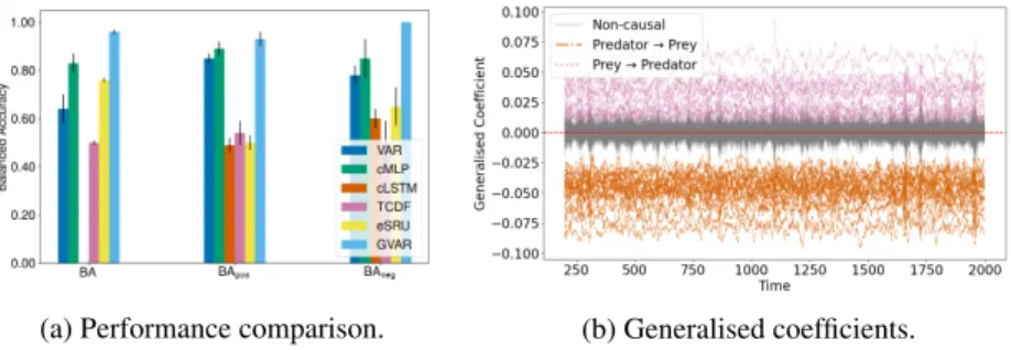
Figure 1 shows the results for this experiment. Our model () considerably outperforms all baselines in detecting effect signs, achieving nearly perfect scores: it infers more meaningful and interpretable parameter values. Figure 1b provides a visualisation of generalised coefficients inferred by GVAR for one simulation of the system. Appendix H contains another effect sign detection experiment on a trivial linear benchmark, which yields similar results.

(a) Performance comparison. (b) Generalised coefficients.

Figure 1: Inference results for the multi-species Lotka–Volterra system.

Baseline methods rely on interpreting weights of relevant layers that, in general, do not need to be associated with effect signs and are only informative about the presence or absence of GC interactions.

Since the GVAR model follows a form of SENNs, its generalised coefficients shed more light into how the future of target variables depends on the past of their predictors. This restricted structure is more intelligible and yet is sufficiently flexible to perform on par with sparse-input neural networks.

5 Conclusion

In this paper, we focused on two problems: (i) inferring GC relationships in multivariate time series under nonlinear dynamics and (ii) inferring signs of GC relationships. We proposed a novel GC inference framework based on autoregressive modelling with SENNs and demonstrated that, on simulated data, its performance is promisingly competitive with the related methods. Our framework performs a stability-based selection of significant relationships, finding a GC structure that is stable on original and time-reversed data. Additionally, it is more amenable to interpretation, since relationships between variables can be explored by inspecting generalised coefficients, which, as we showed empirically, are more informative than input layer weights. In future research, we plan a thorough investigation of the stability-based thresholding procedure and of time-reversal for inferring GC.

Furthermore, we would like to facilitate a more comprehensive comparison with the baselines on real-world data sets. Last but not least, we plan to tackle the problem of inferring time-varying GC structures with the introduced framework.

Broader Impact

This paper presents a novel framework for inferring nonlinear multivariate Granger causality, and its contributions are purely conceptual and experimental. The approach described herein does not have immediate benefits and consequences for the society. The inference framework could be adopted by practitioners from various domains, where inferring Granger causality is of interest, e.g.

for exploratory analysis of time series data. As for any other Granger-causal inference technique, inference results need to be interpreted with caution, while keeping in mind fundamental limitations and assumptions of the framework proposed by C.W.J. Granger. In particular, Granger causality can yield erroneous conclusions under unobserved confounding, instantaneous interactions, and/or insufficient sampling rates.

Acknowledgments and Disclosure of Funding

We thank Ðor ¯de Miladinovi´c for valuable discussions and inputs. We also acknowledge Jonas Rothfuss and Kieran Chin-Cheong for their helpful feedback on the manuscript.

References

[1] D. Alvarez-Melis and T. Jaakkola. Towards robust interpretability with self-explaining neural networks. In Advances in Neural Information Processing Systems 31, pages 7775–7784. Curran Associates, Inc., 2018.

[2] M. O. Appiah. Investigating the multivariate Granger causality between energy consumption, economic growth and CO2emissions in Ghana.Energy Policy, 112:198–208, 2018.

[3] A. Arnold, Y. Liu, and N. Abe. Temporal causal modeling with graphical Granger methods. InProceedings of the 13th ACM SIGKDD international conference on Knowledge discovery and data mining – KDD’07.

ACM Press, 2007.

[4] N. Bacaër. Lotka, Volterra and the predator–prey system (1920–1926). InA Short History of Mathematical Population Dynamics, pages 71–76. Springer London, London, 2011.

[5] A. Ben-Hur, A. Elisseeff, and I. Guyon. A stability based method for discovering structure in clustered data.Pacific Symposium on Biocomputing, pages 6–17, 2002.

[6] Y. Benjamini and Y. Hochberg. Controlling the false discovery rate: A practical and powerful approach to multiple testing.Journal of the Royal Statistical Society. Series B (Methodological), 57(1):289–300, 1995.

[7] K. H. Brodersen, C. S. Ong, K. E. Stephan, and J. M. Buhmann. The balanced accuracy and its posterior distribution. In2010 20th International Conference on Pattern Recognition, pages 3121–3124, 2010.

[8] A. K. Charakopoulos, G. A. Katsouli, and T. E. Karakasidis. Dynamics and causalities of atmospheric and oceanic data identified by complex networks and Granger causality analysis.Physica A: Statistical Mechanics and its Applications, 495:436–453, 2018.

[9] C. W. J. Granger. Investigating causal relations by econometric models and cross-spectral methods.

Econometrica, 37(3):424–438, August 1969.

[10] K. Inoue, A. Doncescu, and H. Nabeshima. Hypothesizing about causal networks with positive and negative effects by meta-level abduction. In P. Frasconi and F. A. Lisi, editors,Inductive Logic Programming, pages 114–129, Berlin, Heidelberg, 2011. Springer Berlin Heidelberg.

[11] A. Karimi and M. R. Paul. Extensive chaos in the Lorenz-96 model.Chaos: An interdisciplinary journal of nonlinear science, 20(4):043105, 2010.

[12] S. Khanna and V. Y. F. Tan. Economy statistical recurrent units for inferring nonlinear Granger causality.

InInternational Conference on Learning Representations, 2020.

[13] T. Kipf, E. Fetaya, K.-C. Wang, M. Welling, and R. Zemel. Neural relational inference for interacting systems. InProceedings of the 35th International Conference on Machine Learning, volume 80 of Proceedings of Machine Learning Research, pages 2688–2697, Stockholmsmässan, Stockholm Sweden, 10–15 Jul 2018. PMLR.

[14] T. Lange, M. L. Braun, V. Roth, and J. M. Buhmann. Stability-based model selection. InAdvances in Neural Information Processing Systems, pages 633–642, 2003.

[15] E. N. Lorenz. Predictability: a problem partly solved. InSeminar on Predictability, volume 1, pages 1–18, Shinfield Park, Reading, 1995.

[16] S. Löwe, D. Madras, R. Zemel, and M. Welling. Amortized causal discovery: Learning to infer causal graphs from time-series data, 2020. arXiv:2006.10833.

[17] H. Lütkepohl.New Introduction to Multiple Time Series Analysis. Springer, 2007.

[18] D. Marinazzo, M. Pellicoro, and S. Stramaglia. Kernel method for nonlinear Granger causality.Physical Review Letters, 100(14), 2008.

[19] J. M. McCracken. Exploratory causal analysis with time series data.Synthesis Lectures on Data Mining and Knowledge Discovery, 8(1):1–147, 2016.

[20] N. Meinshausen and P. Bühlmann. Stability selection.Journal of the Royal Statistical Society: Series B (Statistical Methodology), 72(4):417–473, 2010.

[21] A. Montalto, S. Stramaglia, L. Faes, G. Tessitore, R. Prevete, and D. Marinazzo. Neural networks with non-uniform embedding and explicit validation phase to assess Granger causality. Neural Networks, 71:159–171, 2015.

[22] M. Nauta, D. Bucur, and C. Seifert. Causal discovery with attention-based convolutional neural networks.

Machine Learning and Knowledge Extraction, 1:312–340, 2019.

[23] W. B. Nicholson, D. S. Matteson, and J. Bien. VARX-L: Structured regularization for large vector autoregressions with exogenous variables.International Journal of Forecasting, 33(3):627–651, 2017.

[24] N. Parikh and S. Boyd. Proximal algorithms.Foundations and Trends in optimization, 1(3):127–239, 2014.

[25] J. Peters, D. Janzing, and B. Schölkopf. Causal inference on time series using restricted structural equation models. InAdvances in Neural Information Processing Systems 26, pages 154–162. Curran Associates, Inc., 2013.

[26] J. Peters, D. Janzing, and B. Schölkopf. Elements of Causal Inference – Foundations and Learning Algorithms. The MIT Press, 2017.

[27] W. Ren, B. Li, and M. Han. A novel Granger causality method based on HSIC-Lasso for revealing nonlinear relationship between multivariate time series. Physica A: Statistical Mechanics and its Applications, 541:123245, 2020.

[28] A. Roebroeck, E. Formisano, and R. Goebel. Mapping directed influence over the brain using Granger causality and fMRI.NeuroImage, 25(1):230–242, 2005.

[29] S. M. Smith, K. L. Miller, G. Salimi-Khorshidi, M. Webster, C. F. Beckmann, T. E. Nichols, J. D. Ramsey, and M. W. Woolrich. Network modelling methods for FMRI.NeuroImage, 54(2):875–891, 2011.

[30] W. Sun, J. Wang, and Y. Fang. Consistent selection of tuning parameters via variable selection stability.

Journal of Machine Learning Research, 14(1):3419–3440, 2013.

[31] A. Tank, I. Covert, N. Foti, A. Shojaie, and E. Fox. Neural Granger causality for nonlinear time series, 2018. arXiv:1802.05842.

[32] Y. Wang, K. Lin, Y. Qi, Q. Lian, S. Feng, Z. Wu, and G. Pan. Estimating brain connectivity with varying-length time lags using a recurrent neural network.IEEE Transactions on Biomedical Engineering, 65(9):1953–1963, 2018.

[33] I. Winkler, D. Panknin, D. Bartz, K.-R. Muller, and S. Haufe. Validity of time reversal for testing Granger causality.IEEE Transactions on Signal Processing, 64(11):2746–2760, 2016.

[34] T. Wu, T. Breuel, M. Skuhersky, and J. Kautz. Discovering nonlinear relations with minimum predictive information regularization, 2020. arXiv:2001.01885.

Supplemental Material: Interpretable Models for Granger Causality Using Self-explaining Neural Networks

A Linear Vector Autoregression

Linear vector autoregression (VAR) [17] is a time series model conventionally used to test for Granger causality (see Section 2). VAR assumes linear dynamics:

xt=ν+

K

X

k=1

Ψkx_t−k+εt, (5) whereν ∈R^pis the intercept vector;Ψ_k ∈ R^p×pare coefficient matrices; andε_t ∼ N_p(0,Σ_ε) are Gaussian innovation terms. ParameterKis the order of the VAR model and determines the maximum lag at which Granger-causal interactions occur. In VAR, Granger causality is defined by zero constraints on the coefficients, in particular, xⁱdoes not Granger-cause x^jif and only if, for all lagsk∈ {1,2, ..., K},(Ψk)_j,i = 0. These constraints can be tested by performing, for example, F-test or Wald test.

Usually a VAR model is fitted using multivariate least squares. In high-dimensional time series, regularisation can be introduced to avoid inferring spurious associations. Table 2 shows various sparsity-inducing penalties for a linear VAR model of orderK(see Equation 5), described in [23].

Different penalties induce different sparsity patterns in coefficient matricesΨ1,Ψ2, ...,ΨK. These penalties can be adapted to the GVAR model as the sparsity-inducing term.

Table 2: Various sparsity-inducing penalty terms, described in [23], for a linear VAR of or- der K. Herein, Ψ = [Ψ1 Ψ2 ... ΨK] ∈ R^p×Kp (cf. Equation 5), and Ψk:K = [Ψ_k Ψ_k+1 ... Ψ_K]. Different penalties induce different sparsity patterns in coefficient ma- trices.

Model Structure Penalty

Basic Lasso kΨk₁

Elastic net αkΨk₁+ (1−α)kΨk²₂, α∈(0,1)

Lag group PK

k=1kΨkk_F

Componentwise Pp

i=1

PK k=1

(Ψk:K)_i 2

Elementwise Pp

i=1

Pp j=1

PK k=1

(Ψk:K)_i,j 2

Lag-weighted Lasso PK

k=1k^αkΨkk₁, α∈(0,1)

B Inferring Granger Causality under Nonlinear Dynamics

Below we provide a more detailed overview of the related work on inferring nonlinear multivariate Granger causality, focusing on the recent machine learning techniques that tackle this problem.

Kernel-based Methods. Kernel-based GC inference techniques provide a natural extension of the VAR model, described in Appendix A, to nonlinear dynamics. Marinazzo et al. [18] leverage reproducing kernel Hilbert spaces to infer linear Granger causality in an appropriate transformed feature space. Ren et al. [27] introduce a kernel-based GC inference technique that relies on regularisation – Hilbert–Schmidt independence criterion (HSIC) Lasso GC.

Neural Networks with Non-uniform Embedding. Montalto et al. [21] propose neural networks with non-uniform embedding (NUE). Significant Granger causes are identified using the NUE, a feature selection procedure. An MLP is ‘grown’ iteratively by greedily adding lagged predictor components as inputs. Once stopping conditions are satisfied, a predictor time series is claimed a significant cause of the target if at least one of its lagged components was added as an input. This technique is prohibitively costly, especially, in a high-dimensional setting, since it requires training and comparing many candidate models. Wang et al. [32] extend the NUE by replacing MLPs with LSTMs.

Neural Granger Causality. Tank et al. [31] propose inferring nonlinear Granger causality using structured multilayer perceptron and long short-term memory with sparse input layer weights, cMLP

and cLSTM. To infer GC,pmodels need to be trained with each variable as a response. cMLP and cLSTM leverage the group Lasso penalty and proximal gradient descent [24] to infer GC relationships from trained input layer weights.

Attention-based Convolutional Neural Networks. Nauta et al. [22] introduce the temporal causal discovery framework (TCDF) that utilises attention-based convolutional neural networks (CNN).

Similarly to cMLP and cLSTM [31], the TCDF requires training pneural network models to forecast each variable. Key distinctions of the TCDF are(i)the choice of the temporal convolutional network architecture over MLPs or LSTMs for time series forecasting and(ii)the use of the attention mechanism to perform attribution. In addition to the GC inference, the TCDF can detect time delays at which Granger-causal interactions occur. Furthermore, Nauta et al. [22] provide a permutation-based procedure for evaluating variable importance and identifying significant causal links.

Economy Statistical Recurrent Units. Khanna & Tan [12] propose an approach for inferring nonlinear Granger causality similar to cMLP and cLSTM [31]. Likewise, they penalise norms of weights in some layers to induce sparsity. The key difference from the work of Tank et al. [31] is the use of statistical recurrent units (SRUs) as a predictive model. Khanna & Tan [12] propose a new sample-efficient architecture – economy-SRU (eSRU).

Minimum Predictive Information Regularisation. Wu et al. [34] adopt an information-theoretic approach to Granger-causal discovery. They introduce learnable corruption, e.g. additive Gaussian noise with learnable variances, for predictor variables and minimise a loss function with minimum predictive information regularisation that encourages the corruption of predictor time series. Similarly to the approaches described in [31, 22, 12], this framework requires trainingpmodels separately.

Amortised Causal Discovery & Neural Relational Inference. Kipf et al. [13] introduce the neural relational inference (NRI) model based on graph neural networks and variational autoencoders. The NRI model disentangles the dynamics and the undirected relational structure represented explicitly as a discrete latent graph variable. This allows pooling time series data with shared dynamics, but varying relational structures. Löwe et al. [16] provide a natural extension of the NRI model to the Granger-causal discovery. They introduce a more general framework of the amortised causal discovery wherein time series replicates have a varying causal structure, but share dynamics. In contrast to the previous methods [31, 22, 12, 34], which in this setting, have to be retrained separately for each replicate, the NRI is trained on the pooled dataset, leveraging shared dynamics.

C Self-explaining Neural Networks

Alvarez-Melis & Jaakkola [1] introduce self-explaining neural networks (SENN) – a class of intrinsi- cally interpretable models motivated by explicitness, faithfulness, and stability properties. A SENN with a link functiong(·)and interpretable basis conceptsh(x) :R^p→R^kfollows the form

f(x) =g(θ(x)1h(x)1, ..., θ(x)kh(x)k), (6) wherex ∈ R^p are predictors; andθ(·)is a neural network withkoutputs. We refer toθ(x)as generalised coefficients for data pointxand use them to ‘explain’ contributions of individual basis concepts to predictions. As defined in [1],g(·),θ(·), andh(·)in Equation 6 need to satisfy:

1. g(·)is monotonic and additively separable in its arguments;

2. _∂z^∂g

i >0withz_i=θ(x)_ih(x)_i, for alli;

3. θ(·)is locally difference-bounded byh(·), i.e. for everyx0, there existδ >0andL∈R s.t. ifkx−x0k< δ, thenkθ(x)−θ(x0)k ≤Lkh(x)−h(x0)k;

4. {h(x)i}^k_i=1are interpretable representations ofx;

5. kis small.

A SENN is trained by minimising the following gradient-regularised loss function, which balances performance with interpretability:

Ly(f(x), y) +λLθ(f(x)), (7) where Ly(f(x), y) is a loss term for the ground classification or regression task; λ > 0 is a regularisation parameter; and Lθ(f(x)) =

∇xf(x)−θ(x)^>J_x^h(x)

₂ is the gradient penalty, whereJ_x^his the Jacobian ofh(·)w.r.t.x. This penalty encouragesf(·)to be locally linear.

D Ablation Study of the Loss Function

We inspect hyperparameter tuning results for the GVAR model on Lorenz 96 [15] and synthetic fMRI time series [29] (see Appendix F) as an ablation study for the loss function proposed (see Equation 3 in Section 3). Figures 2 and 3 show heat maps of BA scores (left) and AUPRCs (right) for different values of parametersλandγfor Lorenz 96 and fMRI datasets, respectively. For the Lorenz 96 system, sparsity-inducing regularisation appears to be particularly important, nevertheless, there is also an increase in BA and AUPRC from a moderate smoothing penalty. For fMRI, we observe considerable performance gains from introducing both the sparsity-inducing and smoothing penalty terms. Given the sparsity of the ground truth GC structure and the scarce number of observations (T = 200), these gains are not unexpected. During preliminary experiments, we ran grid search across wider ranges ofλandγvalues, however, did not observe further improvements from stronger regularisation. In summary, these results empirically motivate the need for two different forms of regularisation leveraged by the GVAR loss function: the sparsity-inducing and smoothing penalty terms.

Figure 2: GVAR hyperparameter grid search results for Lorenz 96 time series (underF = 40) across 5 values ofλ ∈ [0.0,3.0]andγ ∈ [0.0,0.02]. Each cell shows average balanced accuracy (left) and AUPRC (right) across 5 replicates (darkercolours correspond to lower performance) for one hyperparameter configuration.

Figure 3: GVAR hyperparameter grid search results for simulated fMRI time series across 5 values ofλ∈[0.0,3.0]andγ∈[0.0,0.1]. The heat map on the left shows average BA scores, and the heat map on the right – average AUPRCs.

E Stability-based Thresholding

The literature on stability-based model selection is abundant [5, 14, 20, 30]. For example, Ben-Hur et al. [5] propose measuring stability of clustering solutions under perturbations to assess structure in the data and select an appropriate number of clusters. Lange et al. [14] propose a somewhat similar approach. Meinshausen & Bühlmann [20] introduce the stability selection procedure applicable to a wide range of high-dimensional problems: their method guides the choice of the amount of regularisation based on the error rate control. Sun et al. [30] investigate a similar procedure in the context of tuning penalised regression models.

Algorithm 1 provides pseudo-code for the stability-based selection of significant GC relationships described in Section 3.1. This procedure finds a threshold which results in a dependency structure that is stable on original and time-reversed time series [33].

Algorithm 1:Stability-based thresholding.

Input:One replicate of multivariate time series{xt}^T_t=1; regularisation parametersλandγ≥0; model orderK≥1; sequenceα= (α1, ..., αQ),0≤α1< α2< ... < αQ≤1.

Output :EstimateAˆof the adjacency matrix of the GC summary graph.

1 Let{x˜t}^T_t=1be the time-reversed version of{xt}^T_t=1, i.e.{˜x1, ...,x˜T} ≡ {xT, ...,x1}.

2 Letτ(X, α)be the elementwise thresholding operator. For each component ofX,τ(Xi,j, α) = 1, if

|Xi,j| ≥α, andτ(Xi,j, α) = 0, otherwise.

3 Train an orderKGVAR with parametersλandγby minimising loss in Equation 3 (see Section 3) on {xt}^T_t=1and computeSas in Equation 4 (see Section 3).

4 Train another GVAR on{x˜t}^T_t=1and computeS˜as in Equation 4 (see Section 3).

5 fori= 1toQdo

6 Letκi=qα_i(S)andκ˜i=qα_i( ˜S), whereqα(X)denotes theα-quantile ofX.

7 Evaluate agreementςi=¹₂h BA

τ(S, κi), τ S˜^>,˜κi

+BA

τ S˜^>,κ˜i

, τ(S, κi)i , where BA(·,·)denotes the balanced accuracy score.

8 end

9 Leti^∗= arg max1≤i≤Qςiandα^∗=αi^∗.

10 LetAˆ=τ(S, qα^∗(S)).

11 returnA.ˆ

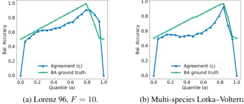
Figure 4 shows an example of agreement between dependency structures inferred on original and time-reversed synthetic sequences across a range of thresholds (see Algorithm 1). In addition, we plot the BA score for resulting thresholded matrices evaluated against the true adjacency matrix. As can be seen, the peak of stability agrees with the highest BA achieved. In both cases, the procedure described by Algorithm 1 chooses the optimal thresholdα_i, which results in the highest agreement with the true dependency structure (unknown at the time of inference).

(a) Lorenz 96,F = 10. (b) Multi-species Lotka–Volterra.

Figure 4: Agreement (N) between GC structures inferred on the original and time-reversed data across a range of thresholds for one simulation of the Lorenz 96 (a) and multi-species Lotka–Volterra (b) systems. BA score (×) is evaluated against the ground truth adjacency matrix.

F Datasets

Herein, we provide a brief summary of synthetic datasets used in our experiments (see Section 4).

Lorenz 96 Model. Lorenz 96 [15] is a standard benchmark for the evaluation of GC inference techniques [31, 12]. This continuous time dynamical system inpvariables is given by the following nonlinear differential equations:

dxⁱ

dt = xⁱ⁺¹−xⁱ⁻²

xⁱ⁻¹−xⁱ+F, for1≤i≤p, (8)

where x⁰ :=x^p, x⁻¹ :=x^p−1, and x^p+1 :=x¹; andF is a forcing constant that, in combination withp, controls the nonlinearity of the system [31, 11]. As can be seen from Equation 8, the true causal structure is quite sparse (the adjacency matrix of the summary graph for this and other datasets is visualised in Figure 5). For our experiments, we numerically simulatedR= 5replicates with p= 20variables andT = 500observations underF= 10. We also experimented withF = 40and observed similar results (see Appendix H).

fMRI. Another dataset we considered consists of rich and realistic simulations of blood-oxygen- level-dependent (BOLD) time series [29] that were generated using the dynamic causal modelling functional magnetic resonance imaging (fMRI) forward model¹. In these time series, variables represent ‘activity’ in different spatial regions of interest within the brain. We considerR = 5 replicates from the simulation no. 3 of the original dataset. These time series containp= 15variables and onlyT = 200observations. The ground truth causal structure is very sparse (see Figure 5).

Lotka–Volterra Model. We consider the Lotka–Volterra model with multiple species Bacaër [4] provides a definition of the original two-species system

, given by the following differential equations:

dxⁱ

dt =αxⁱ−βxⁱ X

j∈P a(xⁱ)

y^j−η xⁱ²

, for1≤i≤p, (9)

dy^j

dt =δy^j X

k∈P a(y^j)

x^k−ρy^j, for1≤j≤p, (10)

where xⁱ correspond to population sizes of prey species; y^j denote population sizes of predator species²;α, β, η, δ, ρ > 0 are fixed parameters controlling strengths of interactions; andP a(xⁱ), P a(y^j)are sets of Granger-causes of xⁱand y^j, respectively. According to Equations 9 and 10, the population size of each prey species xⁱis driven down by

P a(xⁱ)

predator species (negative effects), whereas each predator species y^jis driven up by

P a(y^j)

prey populations (positive effects).

For experiments, we simulated the system underα=ρ = 1.1,β = δ= 0.2,η = 2.75×10⁻⁵, P a(xⁱ)

= P a(y^j)

= 2,p= 10, i.e. 2p= 20variables in total, withT = 2000observations.

Figure 6 depicts signs of GC effects between variables in a multi-species Lotka–Volterra with2p= 20 species and 2 parents per variable. Numerical simulations use the Runge-Kutta method³. We make a few adjustments to the state transition equations, in particular: we introduce normally-distributed innovation terms to make simulated data noisy; during state transitions, we clip all population sizes below 0.

1The data are available athttps://www.fmrib.ox.ac.uk/datasets/netsim/.

2In our simulations, we restricted population sizes xⁱand y^jto be non-negative.

3Simulations are based on the implementation available at https://github.com/smkalami/

lotka-volterra-in-python.

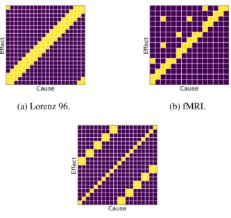
(a) Lorenz 96. (b) fMRI.

(c) Multi-species Lotka–Volterra.

Figure 5: Adjacency matrices of Granger-causal summary graphs for Lorenz 96, simulated fMRI, and multi-species Lotka–Volterra time series.Darkcells correspond to the absence of a GC relationship, i.e.Ai,j= 0;lightcells denote a GC relationship, i.e.Ai,j = 1.

Figure 6: Signs of GC relationships between variables in the Lotka–Volterra system given by Equations 9 and 10, with p = 10. First ten columns correspond to prey species, whereas the last ten correspond to predators. Each prey species is ‘hunted’ by two predator species, and each predator species ‘hunts’ two prey species. Similarly to the other experiments, we ignore self-causal relationships.

G Hyperparameter Tuning

In our experiments (see Section 4), for all of the inference techniques compared, we searched across a grid of hyperparameters that control the sparsity of inferred GC structures. Other hyperparameters were fine-tuned manually. Final results reported in the paper correspond to the best hyperparameter configurations. With this testing setup, our goal was to fairly compare best achievable inferential performance of the techniques.

Tables 3, 4, and 5 provide ranges for hyperparameter values considered in each experiment. For cMLP and cLSTM [31], parameterλis the weight of the group Lasso penalty; for TCDF [22], significance parameterαis used to decide which potential GC relationships are significant; eSRU [12] has three different penalties weighted byλ1:3. For the stability-based thresholding (see Algorithm 1) in GVAR, we used 20 equally spaced values in[0,1]as sequenceα⁴. For Lorenz 96 and fMRI experiments, grid search results are plotted in Figures 2, 7, and 3. Figure 8 contains GVAR grid search results for the Lotka–Volterra experiment.

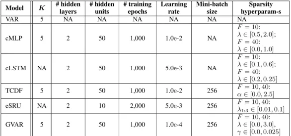
Table 3: Hyperparameter values for Lorenz 96 datasets withF = 10and40. Herein,Kdenotes model order (maximum lag). If a hyperparameter is not applicable to a model, the corresponding entry is marked by ‘NA’.

Model K # hidden layers

# hidden units

# training epochs

Learning rate

Mini-batch size

Sparsity hyperparam-s

VAR 5 NA NA NA NA NA NA

cMLP 5 2 50 1,000 1.0e-2 NA

F= 10:

λ∈[0.5,2.0];

F= 40:

λ∈[0.0,1.0]

cLSTM NA 2 50 1,000 5.0e-3 NA

F= 10:

λ∈[0.1,0.6];

F= 40:

λ∈[0.2,0.25]

TCDF 5 2 50 1,000 1.0e-2 256 F= 10,40:

α∈[0.0,2.5]

eSRU NA 2 10 2,000 5.0e-3 256 F= 10,40:

λ1:3∈[0.01,0.1]

GVAR 5 2 50 1,000 1.0e-4 256

F= 10,40:

λ∈[0.0,3.0], γ∈[0.0,0.025]

Figure 7: GVAR hyperparameter grid search results for Lorenz 96 time series, underF = 10, across 5 values ofλ∈[0.0,3.0]andγ∈[0.0,0.02]. Each cell shows average balanced accuracy (left) and AUPRC (right) across 5 replicates.

4We did not observe high sensitivity of performance w.r.t.α, as long as sufficiently many evenly spaced sparsity levels are considered.

Table 4: Hyperparameter values for simulated fMRI time series.

Model K # hidden layers

# hidden units

# training epochs

Learning rate

Mini-batch size

Sparsity hyperparam-s

VAR 1 NA NA NA NA NA NA

cMLP 1 1 50 2,000 1.0e-2 NA λ∈[0.001,0.75]

cLSTM NA 1 50 1,000 1.0e-2 NA λ∈[0.05,0.3]

TCDF 1 1 50 2,000 1.0e-3 256 α∈[0.0,2.0]

eSRU NA 2 10 2,000 1.0e-3 256

λ1∈[0.01,0.05], λ2∈[0.01,0.05], λ3∈[0.01,1.0]

GVAR 1 1 50 1,000 1.0e-4 256 λ∈[0.0,3.0],

γ∈[0.0,0.1]

Table 5: Hyperparameter values for multi-species Lotka–Volterra time series.

Model K # hidden layers

# hidden units

# training epochs

Learning rate

Mini-batch size

Sparsity hyperparam-s

VAR 1 NA NA NA NA NA NA

cMLP 1 2 50 2,000 5.0e-3 NA λ∈[0.2,0.4]

cLSTM NA 2 50 1,000 5.0e-3 NA λ∈[0.0,1.0]

TCDF 1 2 50 2,000 1.0e-2 64 α∈[0.0,2.0]

eSRU NA 2 10 2,000 1.0e-3 256

λ1∈[0.01,0.05], λ2∈[0.01,0.05], λ3∈[0.01,1.0]

GVAR 1 2 50 500 1.0e-4 256 λ∈[0.0,1.0],

γ∈[0.0,0.01]

(a) BA (b) AUPRC

(c) BApos (d) BAneg

Figure 8: GVAR hyperparameter grid search results for multi-species Lotka–Volterra time series across 5 values ofλ∈[0.0,1.0]andγ∈[0.0,0.01]. Heat maps above show balanced accuracies (a), AUPRCs (b), and balanced accuracies for positive (c) and negative (d) effects.

H Additional Experiments

Inferring Granger Causality: Lorenz 96,F = 40. In addition to the results on the Lorenz 96 system underF= 10(see Section 4), we compared the methods underF= 40. This forcing constant value (in combination withp= 20) results in a higher degree of nonlinearity. In this scenario, our model oce again performs competetively with the baselines (see Table 6).

Table 6: Performance comparison on the Lorenz 96 model withF = 40. Model BA(±SD) AUPRC(±SD)

VAR 0.59(±0.03) 0.47(±0.04) cMLP 0.81(±0.02) 0.96(±0.03) cLSTM 0.66(±0.04) 0.39(±0.06) TCDF 0.60(±0.03) 0.31(±0.05) eSRU 0.89(±0.02) 0.83(±0.03) GVAR 0.89(±0.05) 0.92(±0.02)

Effect Sign Detection in a Linear VAR. Herein we provide results for the evaluation of GVAR and our inference framework on a very simple synthetic time series dataset. We simulate time series with p= 4variables and linear interaction dynamics given by the following equations:

xt=a1xt−1+ε^x_t,

wt=a₂wt−1+a₃xt−1+ε^w_t, y_t=a4y_t−1+a5w_t−1+ε^y_t,

zt=a6zt−1+a7wt−1+a8y_t−1+ε^z_t,

(11)

where coefficientsai∼ U([−0.8,−0.2]∪[0.2,0.8])are sampled independently in each simulation;

andε^·_t∼ N(0,0.16)are additive innovation terms. This is an adapted version of one of artificial datasets described in [25], but without instantaneous effects.

The GC summary graph of the system is visualised in Figure 9. It is considerably denser than for the Lorenz 96, fMRI, and Lotka–Volterra time series investigated in Section 4.

Figure 9: The adjacency matrix of the GC summary graph for the model given by Equation 11.

Similarly to the experiment described in Section 4.2, we infer GC relationships with the proposed framework and evaluate inference results against the true dependency structure and effect signs. Table 7 contains average performance across 10 simulations achieved by GVAR with hyperparameter valuesK= 1,λ= 0.2, andγ= 0.5. In addition, we provide results for some of the baselines (no systematic hyperparameter tuning was performed for this experiment).

GVAR attains perfect AUROC and AUPRC in all 10 simulations. In some cases, stability-based thresholding fails to recover a completely correct GC structure, nevertheless, average accuracy and balanced accuracy scores are satisfactory. Signs of inferred generalised coef- ficients mostly agree with the ground truth effect signs, as given by coefficientsa1:8in Equation 11. Figure 10 shows generalised coef- ficients plotted against time. As expected, coefficients almost do not vary, since parameterγis set to a large value.

Not surprisingly, linear VAR performs the best on this dataset w.r.t. all evaluation metrics. Both cMLP and eSRU successfully infer GC relationships, achieving results comparable to GVAR. However, neither infers effect signs as well as GVAR. Thus, similarly to the experiment in Section 4.2, we conclude that generalised coefficients are more interpretable than neural network weights leveraged by cMLP, TCDF, and eSRU.

To summarise, this simple experiment serves as a sanity check and shows that our GC inference framework performs reasonably in low-dimensional time series with linear dynamics and a relatively dense GC summary graph (cf. Figure 5). Generally, the method successfully infers both the dependency structure and interaction signs.

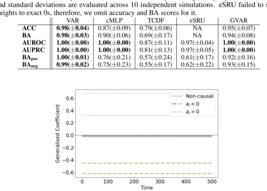
Table 7: Performance on synthetic time series with linear dynamics, given by Equation 11. Averages and standard deviations are evaluated across 10 independent simulations. eSRU failed to shrink weights to exact 0s, therefore, we omit accuracy and BA scores for it.

VAR cMLP TCDF eSRU GVAR

ACC 0.98(±0.04) 0.87(±0.09) 0.79(±0.06) NA 0.95(±0.07) BA 0.98(±0.03) 0.90(±0.06) 0.69(±0.17) NA 0.94(±0.08) AUROC 1.00(±0.00) 1.00(±0.00) 0.87(±0.11) 0.97(±0.04) 1.00(±0.00) AUPRC 1.00(±0.00) 1.00(±0.00) 0.81(±0.13) 0.97(±0.05) 1.00(±0.00) BApos 1.00(±0.01) 0.76(±0.21) 0.57(±0.24) 0.61(±0.17) 0.92(±0.16) BAneg 0.99(±0.02) 0.75(±0.23) 0.55(±0.17) 0.62(±0.22) 0.93(±0.15)

Figure 10: Variability of GVAR generalised coefficients throughout time for one simulation of the time series with linear dynamics (see Equation 11). Observe that signs of generalised coefficients agree with signs of coefficientsai. Generalised coefficients for Granger non-causal relationships are significantly lower in magnitude. As expected, coefficients vary little w.r.t. time, since parameterγis chosen to be very large.