SUPPORTING INFORMATION APPENDIX

(1)

SUPPORTING INFORMATION

APPENDIX

(2)

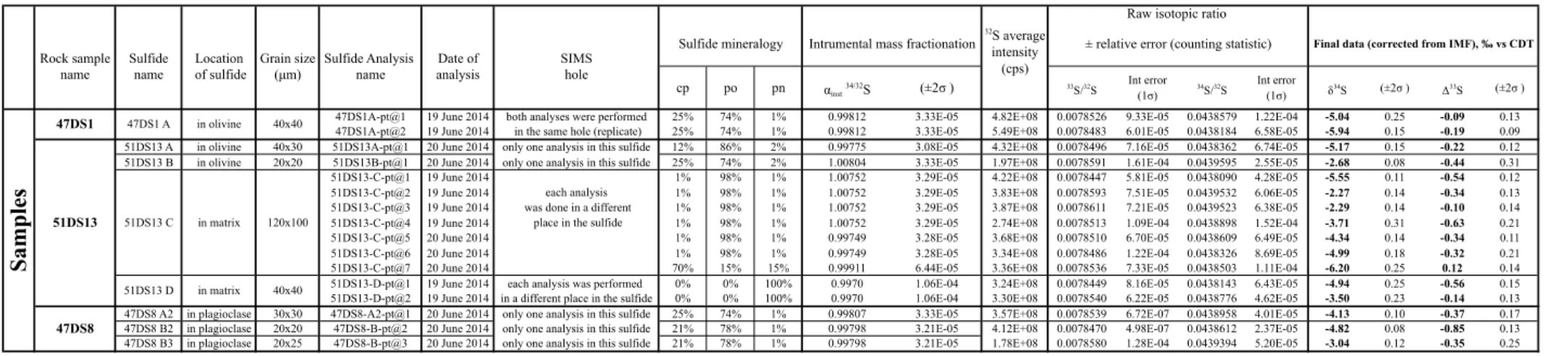
Table S1a: S isotopic analyses

Sulfide mineralogy is expressed as percentages of chalcopyrite (cp, CuFeS2), pentlandite (pn, (Fe,Ni)9S8) and pyrrhotite (po, Fe1-xS).

The measurement sequence was as follows: 17 standards, 2 samples (51DS13, 47DS1), 10 standards (check IMF stability), 2 samples (51DS13A, 51DS13C), 2 standards inside ring (check calibration), 2 samples (51DS13Cabd, 51DS13B, 2 standards inside ring (check calibration)

Rock sample Sulfide Location Grain size Sulfide Analysis Date of SIMS

name name of sulfide (µm) name analysis hole

cp po pn αinst34/32S (±2σ ) ³³S/³²S Int error

(1σ) ³⁴S/³²S Int error

(1σ) δ³⁴S (±2σ ) Δ³³S (±2σ ) 47DS1A-pt@1 19 June 2014 both analyses were performed 25% 74% 1% 0.99812 3.33E-05 4.82E+08 0.0078526 9.33E-05 0.0438579 1.22E-04 -5.04 0.25 -0.09 0.13 47DS1A-pt@2 19 June 2014 in the same hole (replicate) 25% 74% 1% 0.99812 3.33E-05 5.49E+08 0.0078483 6.01E-05 0.0438184 6.58E-05 -5.94 0.15 -0.19 0.09 51DS13 A in olivine 40x30 51DS13A-pt@1 20 June 2014 only one analysis in this sulfide 12% 86% 2% 0.99775 3.08E-05 4.32E+08 0.0078496 7.16E-05 0.0438362 6.74E-05 -5.17 0.15 -0.22 0.12 51DS13 B in olivine 20x20 51DS13B-pt@1 20 June 2014 only one analysis in this sulfide 25% 74% 2% 1.00804 3.33E-05 1.97E+08 0.0078591 1.61E-04 0.0439595 2.55E-05 -2.68 0.08 -0.44 0.31

51DS13-C-pt@1 19 June 2014 1% 98% 1% 1.00752 3.29E-05 4.22E+08 0.0078447 5.81E-05 0.0438090 4.28E-05 -5.55 0.11 -0.54 0.12

51DS13-C-pt@2 19 June 2014 each analysis 1% 98% 1% 1.00752 3.29E-05 3.83E+08 0.0078593 7.51E-05 0.0439532 6.06E-05 -2.27 0.14 -0.34 0.13

51DS13-C-pt@3 19 June 2014 was done in a different 1% 98% 1% 1.00752 3.29E-05 3.87E+08 0.0078611 7.21E-05 0.0439523 6.38E-05 -2.29 0.14 -0.10 0.14

51DS13-C-pt@4 19 June 2014 1% 98% 1% 1.00752 3.29E-05 2.74E+08 0.0078513 1.09E-04 0.0438898 1.52E-04 -3.71 0.31 -0.63 0.21

51DS13-C-pt@5 20 June 2014 1% 98% 1% 0.99749 3.28E-05 3.68E+08 0.0078510 6.70E-05 0.0438609 6.49E-05 -4.34 0.14 -0.34 0.11

51DS13-C-pt@6 20 June 2014 1% 98% 1% 0.99749 3.28E-05 3.34E+08 0.0078486 1.22E-04 0.0438326 8.69E-05 -4.99 0.18 -0.32 0.21

51DS13-C-pt@7 20 June 2014 70% 15% 15% 0.99911 6.44E-05 3.36E+08 0.0078536 7.33E-05 0.0438503 1.11E-04 -6.20 0.25 0.12 0.14

51DS13-D-pt@1 19 June 2014 each analysis was performed 0% 0% 100% 0.9970 1.06E-04 3.24E+08 0.0078449 8.16E-05 0.0438143 6.43E-05 -4.94 0.25 -0.56 0.15 51DS13-D-pt@2 19 June 2014 in a different place in the sulfide 0% 0% 100% 0.9970 1.06E-04 3.30E+08 0.0078540 6.22E-05 0.0438776 4.62E-05 -3.50 0.23 -0.14 0.13 47DS8 A2 in plagioclase 30x30 47DS8-A2-pt@1 20 June 2014 only one analysis in this sulfide 25% 74% 1% 0.99807 3.33E-05 3.57E+08 0.0078539 6.72E-07 0.0438958 4.01E-05 -4.13 0.10 -0.37 0.17 47DS8 B2 in plagioclase 20x20 47DS8-B-pt@2 20 June 2014 only one analysis in this sulfide 21% 78% 1% 0.99798 3.21E-05 4.12E+08 0.0078470 4.98E-07 0.0438612 2.37E-05 -4.82 0.08 -0.85 0.13 47DS8 B3 in plagioclase 20x25 47DS8-B-pt@3 20 June 2014 only one analysis in this sulfide 21% 78% 1% 0.99798 3.21E-05 1.78E+08 0.0078580 1.28E-04 0.0439394 5.20E-05 -3.04 0.12 -0.35 0.25 Final data (corrected from IMF), ‰ vs CDT

± relative error (counting statistic)

Samples

Sulfide mineralogy Intrumental mass fractionation

47DS8

place in the sulfide 47DS1

32S average intensity

(cps)

51DS13

47DS1 A

51DS13 C

51DS13 D in olivine

Raw isotopic ratio

40x40

120x100

40x40 in matrix

in matrix

(3)

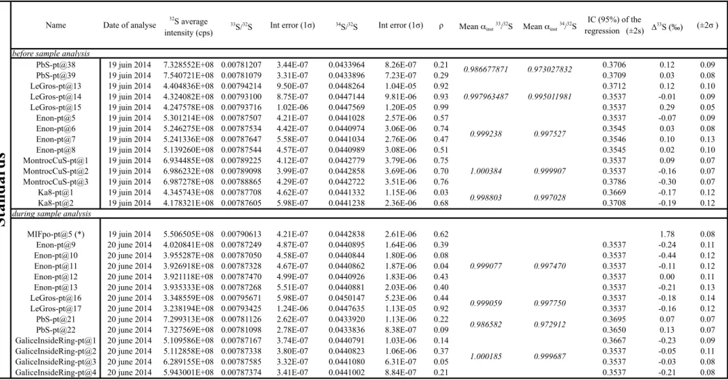
Table S1b: S isotopic analyses on reference material

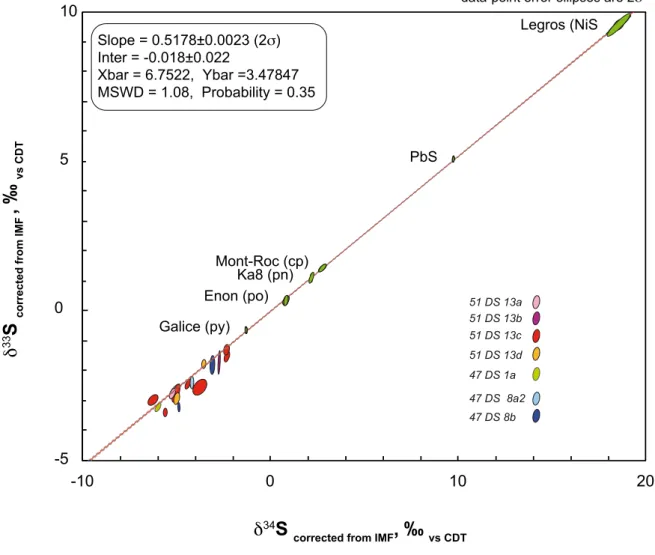
The reference materials define the following correlation: y= 0.50528 (±0.00291)x+ 0.4280 (±0.0286) with x= 103*ln alpha 34 and y= 103*ln alpha 33.

(*) Not used to set up the regression line.

Name Date of analyse ³²S average intensity (cps)

33S/³²S Int error (1σ) ³⁴S/³²S Int error (1σ) ρ Mean αinst33/³²S Mean αinst34/³²S IC (95%) of the

regression (±2s) ∆³³S (‰) (±2σ ) before sample analysis

PbS-pt@38 19 juin 2014 7.328552E+08 0.00781207 3.44E-07 0.0433964 8.26E-07 0.21 0.3706 0.12 0.09

PbS-pt@39 19 juin 2014 7.540721E+08 0.00781079 3.31E-07 0.0433896 7.23E-07 0.29 0.3709 0.03 0.08

LeGros-pt@13 19 juin 2014 4.404836E+08 0.00794214 9.50E-07 0.0448264 1.04E-05 0.92 0.3712 0.12 0.10

LeGros-pt@14 19 juin 2014 4.324082E+08 0.00793100 8.75E-07 0.0447144 9.81E-06 0.93 0.3537 -0.01 0.09

LeGros-pt@15 19 juin 2014 4.247578E+08 0.00793716 1.02E-06 0.0447569 1.20E-05 0.99 0.3537 0.29 0.05

Enon-pt@5 19 juin 2014 5.301214E+08 0.00787507 4.21E-07 0.0441028 2.57E-06 0.57 0.3537 -0.07 0.09

Enon-pt@6 19 juin 2014 5.246275E+08 0.00787534 4.42E-07 0.0440974 3.06E-06 0.74 0.3545 0.03 0.08

Enon-pt@7 19 juin 2014 5.241336E+08 0.00787647 5.58E-07 0.0441034 2.76E-06 0.47 0.3546 0.10 0.13

Enon-pt@8 19 juin 2014 5.139260E+08 0.00787544 4.57E-07 0.0440989 3.08E-06 0.51 0.3545 0.02 0.10

MontrocCuS-pt@1 19 juin 2014 6.934485E+08 0.00789225 4.12E-07 0.0442779 3.79E-06 0.75 0.3537 0.09 0.07

MontrocCuS-pt@2 19 juin 2014 6.986232E+08 0.00789098 3.99E-07 0.0442858 3.69E-06 0.70 0.3537 -0.16 0.07

MontrocCuS-pt@3 19 juin 2014 6.987278E+08 0.00788865 4.29E-07 0.0442722 3.51E-06 0.76 0.3786 -0.30 0.07

Ka8-pt@1 19 juin 2014 4.345743E+08 0.00787708 4.62E-07 0.0441332 1.15E-06 0.03 0.3669 -0.17 0.12

Ka8-pt@2 19 juin 2014 4.178321E+08 0.00787605 5.98E-07 0.0441238 2.36E-06 0.68 0.3708 -0.19 0.12

during sample analysis

MIFpo-pt@5 (*) 19 juin 2014 5.506505E+08 0.00790613 4.21E-07 0.0442838 2.61E-06 0.62 1.78 0.08

Enon-pt@9 20 june 2014 4.020841E+08 0.00787249 4.87E-07 0.0440895 1.64E-06 0.39 0.3537 -0.24 0.11

Enon-pt@10 20 june 2014 3.955287E+08 0.00787050 4.58E-07 0.0440844 1.80E-06 0.08 0.3537 -0.44 0.12

Enon-pt@11 20 june 2014 3.926918E+08 0.00787328 4.67E-07 0.0440862 1.87E-06 0.04 0.3537 -0.11 0.12

Enon-pt@12 20 june 2014 3.921118E+08 0.00787470 4.99E-07 0.0440926 1.83E-06 0.43 0.3537 0.00 0.11

Enon-pt@13 20 june 2014 3.935333E+08 0.00787268 5.51E-07 0.0440881 2.03E-06 0.40 0.3537 -0.21 0.13

LeGros-pt@16 20 june 2014 3.348559E+08 0.00795671 5.98E-07 0.0450147 5.23E-06 0.44 0.3537 -0.18 0.14

LeGros-pt@17 20 june 2014 3.238194E+08 0.00793425 1.24E-06 0.0447635 1.13E-05 0.92 0.3537 -0.16 0.12

PbS-pt@21 20 june 2014 7.299313E+08 0.00781126 2.62E-07 0.0433920 1.13E-06 0.22 0.3695 0.07 0.07

PbS-pt@22 20 june 2014 7.327569E+08 0.00781098 2.78E-07 0.0433836 8.38E-07 0.09 0.3650 0.13 0.07

GaliceInsideRing-pt@1 20 june 2014 5.109586E+08 0.00787167 3.74E-07 0.0440791 1.03E-06 0.14 0.3667 -0.23 0.09

0.999077

0.999059 0.986582

1.000185

0.997470

0.997750 0.972912

0.999687 0.997963487

0.999238

1.000384

0.998803

0.995011981

0.997527

0.999907

0.997028 0.973027832 0.986677871

S tan d ar d s

(4)

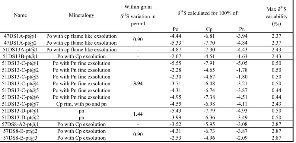
Table S1c: Sulfur isotopic composition of Pitcarin sulfides, mineralogy and within-grain isotopic variation.

An inaccurate correction of the instrumental mass fractionation would lead to misevaluated internal isotopic fractionation.

However, as shown in the last column, the maximum error that could be attributed to inappropriate data treatment is smaller than the actual isotopic range, suggesting that the within-grain variability is signicantly different from 0‰.

Po Cp Pn

47DS1A-pt@1 Po with cp flame like exsolution -4.44 -6.81 -3.94 2.37

47DS1A-pt@2 Po with cp flame like exsolution -5.33 -7.70 -4.84 2.37

51DS13A-pt@1 Po with cp flame like exsolution - -4.87 -7.30 -4.43 2.43

51DS13B-pt@1 Po with Cp exsolution - -2.07 -4.51 -1.63 2.43

51DS13-C-pt@1 Po with Pn fine exsolution -5.55 -7.91 -5.05 0.50

51DS13-C-pt@7 Cp rim, with po and pn -4.55 -6.98 -4.11 2.43

51DS13-D-pt@1 pn -5.43 -7.79 -4.93 0.50

51DS13-D-pt@2 pn -3.99 -6.36 -3.49 0.50

57DS8-A2-pt@1 Po with Cp exsolution - -3.52 -5.95 -3.08 2.87

57DS8-B-pt@2 Po with Cp exsolution -4.31 -6.73 -3.87 2.87

57DS8-B-pt@3 Po with Cp exsolution -2.53 -4.96 -2.09 2.87

Within grain δ³⁴S variation in

permil

δ³⁴S calculated for 100% of:

0.90

3.94

1.44

0.90

Mineralogy Max δ³⁴S

variability (‰) Name

(5)

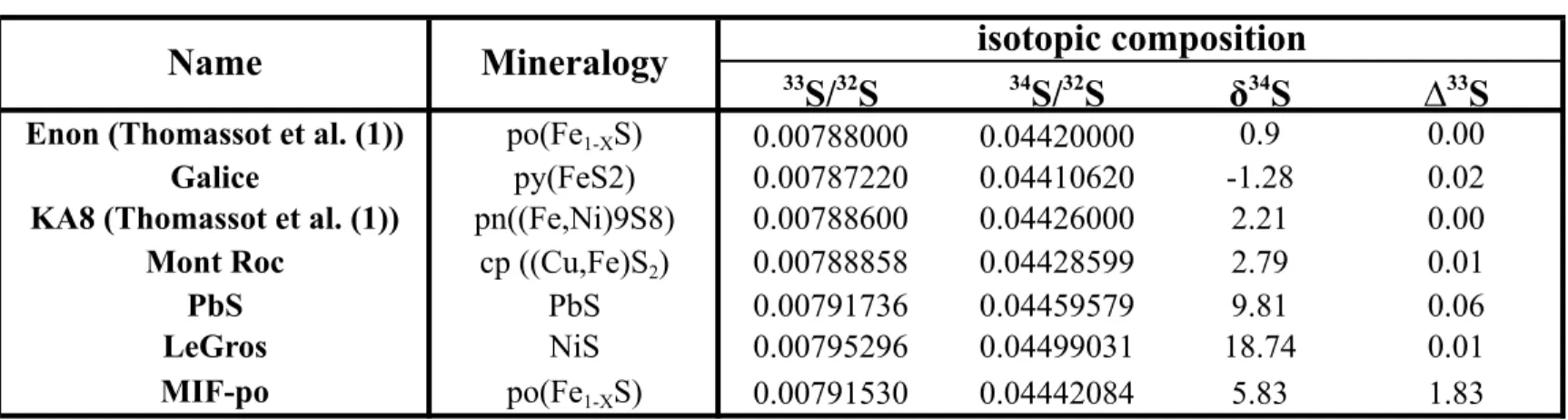
Table S1d: Sulfur reference materials

33S/³²S ³⁴S/³²S δ³⁴S ∆³³S

Enon (Thomassot et al. (1)) po(Fe1-XS) 0.00788000 0.04420000 0.9 0.00

Galice py(FeS2) 0.00787220 0.04410620 -1.28 0.02

KA8 (Thomassot et al. (1)) pn((Fe,Ni)9S8) 0.00788600 0.04426000 2.21 0.00

Mont Roc cp ((Cu,Fe)S₂) 0.00788858 0.04428599 2.79 0.01

PbS PbS 0.00791736 0.04459579 9.81 0.06

LeGros NiS 0.00795296 0.04499031 18.74 0.01

MIF-po po(Fe1-XS) 0.00791530 0.04442084 5.83 1.83

Mineralogy isotopic composition Name

(6)

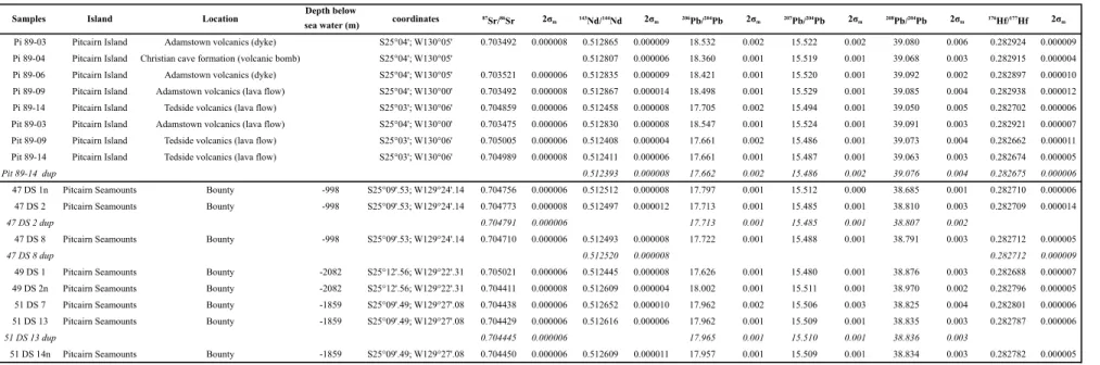
Table S2: Sr, Nd, Pb, and Hf isotopic compositions of Pitcairn samples (Island and Seamounts) from this study. Data shown in italics are duplicates

Depth below sea water (m)

Pi 89-03 Pitcairn Island Adamstown volcanics (dyke) S25°04'; W130°05' 0.703492 0.000008 0.512865 0.000009 18.532 0.002 15.522 0.002 39.080 0.006 0.282924 0.000009

Pi 89-04 Pitcairn Island Christian cave formation (volcanic bomb) S25°04'; W130°05' 0.512807 0.000006 18.360 0.001 15.519 0.001 39.068 0.003 0.282915 0.000004

Pi 89-06 Pitcairn Island Adamstown volcanics (dyke) S25°04'; W130°05' 0.703521 0.000006 0.512835 0.000009 18.421 0.001 15.520 0.001 39.092 0.002 0.282897 0.000010 Pi 89-09 Pitcairn Island Adamstown volcanics (lava flow) S25°04'; W130°00' 0.703492 0.000008 0.512867 0.000014 18.498 0.001 15.529 0.001 39.085 0.004 0.282938 0.000012 Pi 89-14 Pitcairn Island Tedside volcanics (lava flow) S25°03'; W130°06' 0.704859 0.000006 0.512458 0.000008 17.705 0.002 15.494 0.001 39.050 0.005 0.282702 0.000006 Pit 89-03 Pitcairn Island Adamstown volcanics (lava flow) S25°04'; W130°00' 0.703475 0.000006 0.512830 0.000008 18.547 0.001 15.524 0.001 39.091 0.003 0.282921 0.000007 Pit 89-09 Pitcairn Island Tedside volcanics (lava flow) S25°03'; W130°06' 0.705005 0.000006 0.512408 0.000004 17.661 0.002 15.486 0.001 39.073 0.004 0.282662 0.000011 Pit 89-14 Pitcairn Island Tedside volcanics (lava flow) S25°03'; W130°06' 0.704989 0.000008 0.512411 0.000006 17.661 0.001 15.487 0.001 39.063 0.003 0.282674 0.000005

Pit 89-14 dup 0.512393 0.000008 17.662 0.002 15.486 0.002 39.076 0.004 0.282675 0.000006

47 DS 1n Pitcairn Seamounts Bounty -998 S25°09'.53; W129°24'.14 0.704756 0.000006 0.512512 0.000008 17.797 0.001 15.512 0.000 38.685 0.001 0.282710 0.000006

47 DS 2 Pitcairn Seamounts Bounty -998 S25°09'.53; W129°24'.14 0.704773 0.000008 0.512497 0.000012 17.713 0.001 15.485 0.001 38.810 0.003 0.282709 0.000014

47 DS 2 dup 0.704791 0.000006 17.713 0.001 15.485 0.001 38.807 0.002

47 DS 8 dup 0.512520 0.000008 0.282712 0.000009

51 DS 13 dup 0.704445 0.000006 17.965 0.001 15.510 0.001 38.836 0.003

2σm 208Pb/²⁰⁴Pb 2σm 176Hf/¹⁷⁷Hf 2σm 207Pb/²⁰⁴Pb

Samples Island Location coordinates ⁸⁷Sr/⁸⁶Sr 2σm 143Nd/¹⁴⁴Nd 2σm 206Pb/²⁰⁴Pb 2σm

(7)

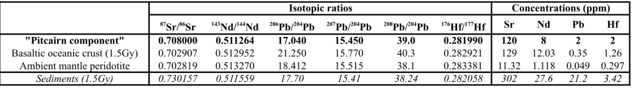
Table S3: Parameters of the mixing model that reproduces the isotopic data of Pitcairn island and seamounts

87Sr/⁸⁶Sr ¹⁴³Nd/¹⁴⁴Nd ²⁰⁶Pb/²⁰⁴Pb ²⁰⁷Pb/²⁰⁴Pb ²⁰⁸Pb/²⁰⁴Pb ¹⁷⁶Hf/¹⁷⁷Hf Sr Nd Pb Hf

"Pitcairn component" 0.708000 0.511264 17.040 15.450 39.0 0.281990 120 8 2 2 Basaltic oceanic crust (1.5Gy) 0.702907 0.512952 21.250 15.770 40.3 0.282921 129 12.03 0.35 1.26

Ambient mantle peridotite 0.702819 0.513270 18.412 15.515 38.1 0.283381 11.32 1.118 0.049 0.297 Sediments (1.5Gy) 0.730157 0.511559 17.70 15.41 38.24 0.282058 302 27.6 21.2 3.42

Isotopic ratios Concentrations (ppm)

Footnotes: The compositions of the 1.5Gy recycled materials (basaltic crust and sediments) and ambient peridotite are from Delavault et al. (2) .

(8)

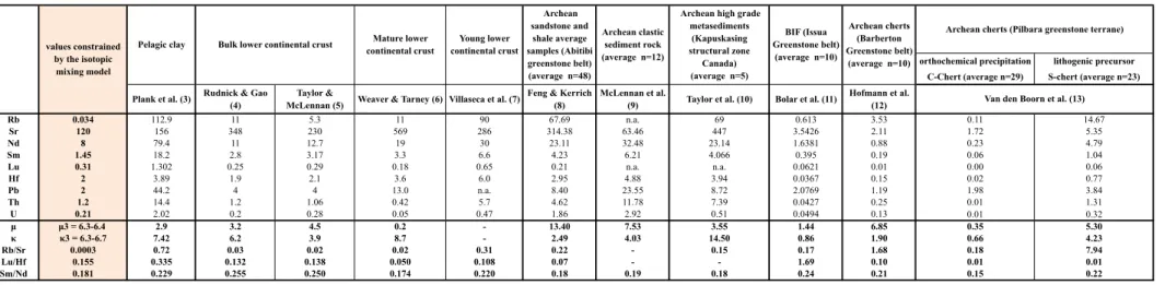
Table S4: Trace element contents (in ppm) of the "Pitcairn component" relative to those of pelagic clay, lower continental crust and various Archean sedimentary materials.

orthochemical precipitation lithogenic precursor C-Chert (average n=29) S-chert (average n=23) Plank et al. (3) Rudnick & Gao

(4)

Taylor &

McLennan (5) Weaver & Tarney (6) Villaseca et al. (7) Feng & Kerrich (8)

McLennan et al.

(9) Taylor et al. (10) Bolar et al. (11) Hofmann et al.

(12)

Rb 0.034 112.9 11 5.3 11 90 67.69 n.a. 69 0.613 3.53 0.11 14.67

Sr 120 156 348 230 569 286 314.38 63.46 447 3.5426 2.11 1.72 5.35

Nd 8 79.4 11 12.7 19 30 23.11 32.48 23.14 1.6381 0.88 0.23 4.79

Sm 1.45 18.2 2.8 3.17 3.3 6.6 4.23 6.21 4.066 0.395 0.19 0.06 1.04

Lu 0.31 1.302 0.25 0.29 0.18 0.65 0.21 n.a. n.a. 0.0621 0.01 0.00 0.06

Hf 2 3.89 1.9 2.1 3.6 6.0 2.95 4.88 3.94 0.0367 0.15 0.02 0.77

Pb 2 44.2 4 4 13.0 n.a. 8.40 23.55 8.72 2.0769 1.19 1.98 3.84

Th 1.2 14.4 1.2 1.06 0.42 5.7 4.62 11.78 7.39 0.0427 0.25 0.01 1.31

U 0.21 2.02 0.2 0.28 0.05 0.47 1.86 2.92 0.51 0.0494 0.13 0.01 0.32

µ µ3 = 6.3-6.4 2.9 3.2 4.5 0.2 - 13.40 7.53 3.55 1.44 6.85 0.35 5.30

κ κ3 = 6.3-6.7 7.42 6.2 3.9 8.7 - 2.49 4.03 14.50 0.86 1.90 0.66 4.23

Rb/Sr 0.0003 0.72 0.03 0.02 0.02 0.31 0.22 - 0.15 0.17 1.68 0.18 7.94

Lu/Hf 0.155 0.335 0.132 0.138 0.050 0.108 0.07 - - 1.69 0.10 0.01 0.01

Sm/Nd 0.181 0.229 0.255 0.250 0.174 0.220 0.18 0.19 0.18 0.24 0.21 0.15 0.22

Bulk lower continental crust Pelagic clay

values constrained by the isotopic

mixing model

Archean clastic sediment rock (average n=12)

Archean cherts (Barberton Greenstone belt)

(average n=10) Mature lower

continental crust

Young lower continental crust

Van den Boorn et al. (13) Archean

sandstone and shale average samples (Abitibi greenstone belt) (average n=48)

Archean high grade metasediments

(Kapuskasing structural zone

Canada) (average n=5)

BIF (Issua Greenstone belt)

(average n=10)

Archean cherts (Pilbara greenstone terrane)

Footnotes: Sr, Nd, Hf and Pb contents required by the curvature of the mixing arrays shown in figures 2 and S3 are listed in the first column while Rb, Sm, Lu, Th, and U contents were calculated to fit the isotopic ratios.

Pelagic sediments may constitute a good candidate to model the Pitcairn source, as they have low ²³⁸U/²⁰⁴Pb and high ²³²Th/²³⁸U, leading with time to low ²⁰⁶Pb/²⁰⁴Pb and high ²⁰⁸Pb/²⁰⁴Pb ratios (3,14). However, they also have high ⁸⁷Rb/⁸⁶Sr (~2.08 see ref.3) that lead, with time, to very high ⁸⁷Sr/⁸⁶Sr, much higher than the value required by our mixing model (our calculated ⁸⁷Rb/⁸⁶Sr is ~0.001).

Lower crust recycled into the mantle has also been suggested to explain the EMI composition. Such material could have the required high ²⁰⁸Pb/²⁰⁴Pb and low ²⁰⁶Pb/²⁰⁴Pb observed in Pitcairn due to its low µ and high κ. However, the other parent/daughter ratios (Rb/Sr, Sm/Nd and Lu/Hf) differ from those constrained by our mixing model and would not produce the necessary Sr, Nd and Hf isotopic ratios.

(9)

1

Figure S1

1

2

Figure S1: Images of the analyzed sulfides. Sub-panels a1, b1, c1, d1, e1 and f1 show reflected-light 3

optical photomicrographs. Panels a2, b2, c2, d2 and e2 show backscattered electron images from the 4

electron microprobe at 20kV. Panels a3, b3, d3 and e3 show enlarged photos of the respective sulfides.

5

Panel c3 shows an SIMS image of sulfide 51DS13C after analysis; in this panel, numbers refer to 6

individual analyses (for example, 1 corresponds to the analysis called 51DS13-C-pt@1 in Table S1).

7

Only sulfides in sample 51DS13C were big enough to perform several analyses at different locations 8

in individual sulfide inclusions. For the other sulfides, the SIMS beam size was similar to the sample 9

size and no SIMS images are provided. Unfortunately, sulfides from samples 51DS13D and 47DS8B 10

were found only during the SIMS analyses session and no microprobe images are available, only 11

sample 47DS8B has a reflected-light optical microscope image shown in panel f₁. The mineralogy and 12

proportion of sulfide types are given in Table S1.

13 14 15 16 17 18 19 20 21

(10)

2

Figure S2

22

23

Figure S2: Pb, Sr, Nd and Hf isotopic compositions showing how our new data compare to previously 24

published data along the Pitcairn-Gambier chain and some other global OIB. (a) ²⁰⁷Pb/²⁰⁴Pb vs.

25 206Pb/²⁰⁴Pb, (b) ²⁰⁸Pb/²⁰⁴Pb vs. ²⁰⁶Pb/²⁰⁴Pb, (c) ¹⁷⁶Hf/¹⁷⁷Hf vs. ¹⁴³Nd/¹⁴⁴Nd and (d) ¹⁴³Nd/¹⁴⁴Nd vs.

26 87Sr/⁸⁶Sr. Literature data: Mururoa(15-18); Fangataufa(16, 17, 19); Gambier(2, 16, 17, 20); Pitcairn 27

Island and seamounts(21-25). Fields for Kerguelen (dark green), Walvis Ridge (light green), Society 28

(beige), Austral-Cook (pink), Marquesas (blue) and Hawaii (purple) are from the GEOROC database.

29 30 31 32 33 34

0.2825 0.2827 0.2829 0.2831 0.2833

0.5122 0.5124 0.5126 0.5128 0.5130 0.5132

38.0 38.4 38.8 39.2 39.6 40.0

17 18 19 20 21

15.4 15.5 15.6 15.7

17 18 19 20 21

0.5123 0.5125 0.5127 0.5129 0.5131

0.702 0.703 0.704 0.705 0.706

a

c

b

d

Mururoa Fangataufa Gambier Pitcairn Island Pitcairn Seamounts

Literature This study

Pitcairn Island Pitcairn Seamounts 208 Pb/204 Pb

207 Pb/204 Pb

87Sr/⁸⁶Sr

206Pb/²⁰⁴Pb ²⁰⁶Pb/²⁰⁴Pb

143 Nd/144 Nd

176 Hf/177 Hf

143Nd/¹⁴⁴Nd

Kerguelen Kerguelen

Kerguelen

Hawaii

Hawaii Hawaii

Walvis Ridge Walvis

Ridge

Walvis Ridge Walvis Ridge

Austral-Cook

Society Society Austral-Cook Society

Austral-Cook Marquesas

Society

Austral-Cook

Marquesas

Marquesas Marquesas

(11)

3

Figure S3

35

36

Figure S3: Mixing arrays similar to those shown in figure 2 but for all isotopic systems. Literature 37

data are shown with diamonds: Mururoa(15-18) (blue), Fangataufa(16, 17, 19) (purple), Gambier(2, 38

16, 17, 20) (green), Pitcairn Island and seamounts(21-25) (orange and red).

39 40 41 42 43 44 45 46 47 48

(12)

4

Figure S4

49

50 51

Figure S4: Theoretical evolution of Pb isotopes through time in ²⁰⁷Pb/²⁰⁴Pb versus ²⁰⁶Pb/²⁰⁴Pb space 52

showing the individual stages of the Monte Carlo refinement model used to reach the present-day Pb 53

isotopic composition of the Pitcairn component. The model has three steps: (I) the first step, shown by 54

the dark blue curve, starts at the Earth initial ratios (blue cross) and evolves along a line controlled 55

by a µ1 of 8.3 (26). This corresponds to the evolution of the Earth´s initial mantle. (II) The second step 56

represents the crustal history. It starts at T2 and the Pb isotopic composition shown with the red cross 57

evolves along the red curve. (III) The third step represents the sedimentary history. It starts at T₃ and 58

the Pb isotopic ratios evolve along the green curve and reach the ‘Pitcairn component’ shown with a 59

yellow star. The parameters µ2, µ3 and T3 (and also κ1 & κ2) are unknown in our model and those 60

parameters are tested with the Monte Carlo refinement method described below.

61 62 63 64 65 66 67 68 69 70 71 72

(μ¹=8.3)

Geochron

T1= Earth formation (4.55Gy)

T

2

=3Gy

Pitcairn component T

₃

Mantle history

206

Pb/

²⁰⁴

Pb

207

Pb/

204

Pb

10 11 12 13 14 15 16 17

9 11 13 15 17 19

Sedimentary Crustal

history history

(13)

5

Figure S5

73

74

Figure S5: Interdependence of the evolution parameters of the three-stage Pb evolution model 75

showing the results for the Monte Carlo refinement modeling. Only the values fitting the target (i.e.

76

the Pitcairn Component) are shown. See method section for details. The pink field highlights ages 77

compatible with the presence of S-MIF. The dashed lines show the preferred range of µ2 (9 - 11.6) 78

and κ2 (4 - 5) for continental crust and the red dots correspond to results assuming such µ2 and κ2. It 79

is clear that the age T₃ (Gy) is highly dependent on µ2 (see panel a). Selecting a possible range of 80

continental crust µ2 value between 9.0 and 11.6 limits T3 to 2.4-2.8 Gy. Once T3 is constrained, it 81

limits the possible range of µ3 (see panel b) and κ3 (see panels c and d), but it is independent of κ2

82

(panel e).

83 84 85 86 87 88 89 90 91 92

(14)

6

Figure S6

93

94

Figure S6: Results of the Monte Carlo refinement modelling for three distinct ages of crustal history 95

onset (T2) of 2.5, 3.0 and 3.5 Ga. Panel (a) shows the interdependence between κ2, µ2 and κ3, panel 96

(b) shows interdependences between µ2, κ2 and T3, panel (c) shows the interdependence between µ2 &

97

κ3 and panel (d) shows the interdependence between µ2 &T3. Only model parameters that produce 98

results within <0.01 of the isotopic ratios of the target ‘Pitcairn component’ (²⁰⁶Pb/²⁰⁴Pb=17.04, 99 207Pb/²⁰⁴Pb=15.45, ²⁰⁸Pb/²⁰⁴Pb=39) are represented (see method section for details). The grey fields in 100

panels a&b show our preferred range of µ2 (9 - 11.6) and κ2 (4 - 5) for continental crust and the red 101

dots show the corresponding results. (e) Proportion of successful results as a function of the age used 102

for the onset of crustal history T2. Color coding is similar to other panels. For completeness, the grey 103

histograms in panel e show the proportion of successful results for T2 values between the three we 104

chose to represent on panels a-d. The total number of successful results is 1.2×e⁵ solutions out of the 105

total of 1×e¹² configurations tested.

106 107

(15)

7

Radiogenic isotope analyses

108

1. Material 109

Samples were collected either in the field (Pitcairn Island) or dredged (Pitcairn Seamounts) 110

during the SO-65 campaign of the German RV "Sonne" in 1989. Sixteen basalts were selected 111

(8 from the island and 8 from a seamount) on freshness criteria. All samples were crushed in 112

an agate mortar.

113 114

2. Analytical methods 115

Nd, Hf, Pb, and Sr were isolated using ion exchange chromatography techniques described in 116

Chauvel et al.(27). The isotopic ratios were measured using high-resolution multicollector 117

ICP-MS (Nu Instrument 1700) at ENS Lyon for Nd, Hf and Pb, and TIMS (Thermo Scientific 118

Triton) at PSO-IUEM in Brest for Sr. The blanks were on average 84 pg for Nd (n=8), 28 pg 119

for Hf (n=5), 76 pg for Pb (n=6), and 23 pg for Sr (n=2). The Hf and Nd isotopic data were 120

corrected for mass fractionation using ¹⁷⁹Hf/¹⁷⁷Hf=0.7325 and ¹⁴⁶Nd/¹⁴⁴Nd=0.7219. The 121

average ¹⁴³Nd/¹⁴⁴Nd obtained for the Nd Ames-Rennes standard was 0.511967±30 (2σ, n=43) 122

and the average ¹⁷⁶Hf/¹⁷⁷Hf obtained for the Hf Ames-Grenoble standard was 0.282156±12 123

(2σ, n=26). Both standards were run every 2 or 3 samples, and any potential drift was 124

corrected using the values published by Chauvel and Blichert-Toft(28) 125

(¹⁴³Nd/¹⁴⁴Nd=0.511961) and Chauvel et al.(27) (¹⁷⁶Hf/¹⁷⁷Hf=0.282160). Lead mass 126

fractionation bias was corrected using a Tl tracer(29) and instrumental drift was corrected 127

using the standard bracketing method, with the NBS981 standard run every 2 or 3 samples 128

and corrections made to the values recommended by Galer and Abouchami(30). The Pb 129

isotopic data were measured over five sessions, and the average ²⁰⁸Pb/²⁰⁴Pb, ²⁰⁷Pb/²⁰⁴Pb and 130

206Pb/²⁰⁴Pb for NBS981 were 36.696±11, 15.491±4 and 16.937±4 (2σ, n=64). Sr isotopic 131

compositions were measured during 2 different sessions. Because the average values obtained 132

for the NBS987 standard differ slightly between the two sessions (0.710241±14 (2σ, n=7);

133

and 0.710231±10 (2σ, n=16), we normalized all measured ⁸⁷Sr/⁸⁶Sr ratios to the 134

recommended value of 0.710250 for the standard.

135 136

Sulfides analyses

137

1. Material 138

(16)

8 The sulfides in Pitcairn lavas are indifferently included in olivine, plagioclase or are directly 139

part of the matrix (see Figure S1). They are polyphase sulfide assemblages containing low-Ni 140

pyrrhotite (po, Fe1-XS), pentlandite (pn, FeNi7S8) and chalcopyrite (cp, CuFeS). The complex 141

mineralogy of these Cu-Fe-Ni sulfides is comparable to sulfide droplets occurring in mafic 142

mantle xenoliths(31) or sulfides included in eclogitic diamonds(1). Experimental studies at 143

temperatures above 300°C have shown that sulfide assemblages in the Cu-Fe-Ni-S system 144

form by sub-solidus exsolution from the monosulfide solid solutions (Mss) stable under 145

mantle conditions. This exsolution occurs long after sulfide entrapment in either olivine or 146

plagioclase (typically from about 560°C for cp(32, 33) and down to 250°C for low-Ni 147

po(34)).

148

The first liquid resulting from the incongruent melting process of the mantle Mss is Cu-rich.

149

A Cu-bearing intermediate solid solution from which cp later crystallizes appears as a phase 150

on the liquidus at about 970°C(35). Pictures of sulfides (Figure S1) show that the chalcopyrite 151

forms rims around the pyrrhotite instead of migrating, demonstrating that the liquid was 152

already trapped in the host minerals and that sulfide grains behave as closed system at least 153

since the temperature dropped below 970°C.

154 155

2. Method 156

We performed the in-situ multiple S-isotopes analyses (δ³³S, δ³⁴S, ∆³³S) using a high- 157

resolution secondary ion mass spectrometer (CAMECA 1280-HR, CRPG-Nancy). The 158

analytical methods and instrument parameters, previously described in Kitayama et al.

159

(2012)(36), were adapted to mantle sulfides. The samples were sputtered with a 1.5 nA Cs+

160

beam resulting in a spot size of about 15 µm. The negative secondary ions were accelerated at 161

10 kV and subsequently filtered in energy and mass. Relative isotope abundances were 162

simultaneously quantified in multicollection mode with three Faraday cups (L2 for ³²S-, C for 163

33S-, and H1 for ³⁴S-). Each measurement consisted of 120s of pre-sputtering (during which 164

the backgrounds of the three Faraday cups were automatically measured) followed by 40 165

measurement cycles of 6 seconds each.

166

Isobaric interferences on the ³³S peak were resolved using entrance slits (60 µm) as well as 167

exit slits (100 µm) that increase the mass resolution power up to 4500.

168 169

2.1 Reference materials 170

The main technical difficulty of in-situ sulfur isotope analysis is related to chemical 171

heterogeneity of the sulfides because each mineral is associated with a specific instrumental 172

(17)

9 mass fractionation (IMF). Consequently, in order to obtain all the IMF data necessary to 173

correct the data, we used a standard collection that includes the main Cu-Fe-Ni sulfide end 174

members: one pyrrhotite (Enon), one pentlandite (Ka8) and one chalcopyrite (Mont Roc). In 175

addition, we used highly fractionated reference materials, which are key standards for 176

calibrating the instrumental mass fractionation line: one galena (PbS), one pyrite (Galice) and 177

one Ni-sulfide (Legros). Finally, we used one additional pyrrhotite sample with a significant 178

S-MIF anomaly (MIF-po). All reference materials are listed in Table S1c.

179 180

Bulk isotope ratios of reference material were measured at the IPGP (Institut de Physique du 181

Globe Paris), using a fluorination line(37) to convert Ag2S into SF6. Gas separation and 182

purification (from condensable species and residual fluorine) was performed using cryogenic 183

trapping and gas chromatography respectively. Purified SF6 was then analyzed using a dual 184

inlet ThermoFinniganMAT 253 isotope ratio mass spectrometer where m/z=127+, 128+, 185

129+ and 131+ ion beams are monitored (a description of the fluorination protocol is 186

provided in Thomassot et al. 2015(38)).

187 188

2.2 In-Situ mass-independent fractionation measurements 189

2.2.1 Definition and notation 190

Sulfur isotopic fractionation factors are classically expressed relatively to the Canyon Diablo 191

Troilite (CDT) composition such that:

192 193

𝛼_!"!"#$%& = !"!/!"!!"#$%&

!"!/!"!!"# and 𝛼_!!= !!!/!"!!"#$%&

!!!/!"!!"#

194

where ³⁴S/³²S and ³³S/³²S are the absolute isotopic ratios and ³⁴S/³²S CDT= 0.0441626 and 195

33S/³²S CDT = 0.00787729, (from Ding et al., 2001(39)) 196

197

Isotopic fractionation would modify these factors according to a mass fractionation law such 198

199 as:

𝛼_!! !"#$%& = 𝛼_!"!"#$%&!

ln𝛼_!! !"#$%& = 𝛽∗𝛼_!"!"#$%& + 𝜀 200

A first order mass fractionation law for sulfur isotope partitioning at equilibrium would define 201

a 𝛽 factor of 0.515. Raw SIMS analyses are related to an instrumental fractionation factor 𝛽′

202

which slighly differs from this theoretical 𝛽 exponent.

203

(18)

10 Mass independent fractionation (∆³³S) refers to deviations from the mass fractionation law 204

(e.g. excess or deficit of ³³S). Effectively, ∆³³S corresponds to the distance of the sample 205

measurement perpendicular to the instrumental fractionation line (IFL), and is expressed in ‰ 206

207 as:

208

Equation 1:

209

∆^!!𝑆 ‰ = 10^!× 𝑙𝑛𝛼_!!!"#$%&"'− 𝛽′𝑙𝑛𝛼_!"!"#$%&"'+𝜀′

210

where β’ represents the slope, 𝜀′ the y-intercept of the IFL and 𝛼_!!!"#$%&"' the raw isotopic 211

ratios normalized to the CDT isotopic ratios (before instrumental mass fractionation , see 212

section 2.3). A collection of reference material of known composition is thus required to 213

define 𝛽^! and 𝜀′ during the analytical session.

214 215

2.2.2 Calculation of ∆³³S, method, corrections and associated error:

216

Seven reference materials, including one mass-independently fractionated pyrrhotite (MIF-po 217

see Table S1) and six grains without significant S-MIF, displaying a large range of sulfur 218

isotopic compositions (δ³⁴S ranging from -1.28 to +18.74 ‰), were used to calibrate the 219

instrumental mass fractionation line of S isotopes during ion probe analyses.

220 221

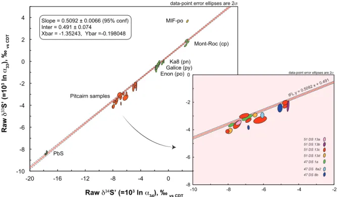
We measured the exponential factor as the slope of the linear regression of the reference 222

material analyses before IMF correction (±2 𝜎 errors related to counting statistic, see Figure 223

S7). For our analytical session, β' = 0.5092 ± 0.0066. The stability of this factor through time 224

(i.e. the stability of the analytical parameters such as the cross-calibration of the detector 225

yields) is the key to reliable in-situ multiple sulfur isotopes analysis. It was monitored by 226

repeated measurements of a grain of reference material (Galice (FeS2), δ³⁴S = -1.28‰). A 227

piece of the Galice standard was mounted in the sample ring, and analyzed between two 228

different sample grains (GaliceInsideRing, n=4, see Table S1b).

229

The ε’ is directly related to the analytical parameters of the detector yields. Long-term 230

stability of this factor was monitored throughout the entire session. We determined that 231

ε’=0.491(±0.074). The reference materials display a small ∆³³S with an average value of - 232

0.02 ‰, an average gap between standard measurements and the fractionation line equal to 233

± 0.14 ‰ (calculated from the root mean square of these ∆³³S, i.e. ^∆^!!^! ^!

! ).

234

(19)

11 The results are in good agreement with the composition determined earlier by classical gas 235

source mass spectrometry (see Table S1d).

236

The calibration error can be determined using the standard error to the mean:

237

Equation 2:

238

𝜎_!"#$% _∆^!!_! = 𝑠𝑡𝑑𝑒𝑣 ∆^!!𝑆

𝑛 239

The internal error on ∆³³S was calculated from the counting statistics on ³⁴S/³²S and ³³S/³²S 240

ratios (with σ_!!" and σ_!!! representing the internal absolute errors, respective) using the 241

partial derivation of Equation 1 such that:

242

Equation 3:

243

𝜎_!"# _∆^!!_! = 10

𝛼_!!

! !

σ_!!!^!+ −𝛽.10 𝛼_!"

! !

σ_!!"^!+ 2𝜌×10^!

𝛼_!!×−𝛽.10^!

𝛼_!" ×σ_!!!×σ_!!"

244

with ρ being the correlation factor between δ³⁴S and δ³³S determined from the counting 245

statistic on ³⁴S/³²S, ³³S/³²S and ³³S/³⁴S, and σ_!!!/!" the internal absolute error on the ³³S/³⁴S 246

ratio such that:

247 248

Equation 5:

249

𝜌 =σ_!!"^!+σ_!!!^!−σ_!!!/!"^! 2×σ_!!!×σ_!!"

250

The resulting 2σ external error on the ∆³³S is then calculated by adding, in a quadratic way, 251

the internal error (Equation 3) and the calibration error (Equation 4) such that:

252

Equation 6:

253

𝜎_!"# _∆^!!_! 2𝜎 =2× 𝜎_!"# _∆^!!_! ^!+𝜎_!"#$% _∆^!!_! ^!

This external error ranges from +0.05 ‰ up to +0.14‰ on reference material (average 254

𝜎_!"# _∆^!!_! = 0.10 ± 0.02 ‰) and from +0.09‰ to +0.31‰ on the samples (0.16 ± 0.06‰ on

255

average). An optimal surface condition of the reference material improves the counting 256

statistics, thus explaining the slight difference between 𝜎_!"# _∆^!!_! in standards and samples.

257

In order to check the validity of these ∆³³S calculation we:

258