Arithmetic Divisors on Products of Curves over non-Archimedean Fields
Dissertation
zur Erlangung des Doktorgrades der Naturwissenschaften (Dr. rer. nat.)
an der Fakult¨ at f¨ ur Mathematik der Universit¨ at Regensburg
Vorgelegt von Philipp Vollmer aus Herford bei Prof. Dr. Klaus K¨ unnemann
Regensburg im Jahre 2016
Die Arbeit wurde angeleitet von Prof. Dr. Klaus K¨unnemann
Pr¨ufungsausschuß:
Vorsitzender: Prof. Dr. Helmut Abels Erster Gutachter: Prof. Dr. Klaus K¨unnemann Zweiter Gutachter: Prof. Dr. Walter Gubler Weiterer Pr¨ufer: Prof. Dr. Felix Finster
Contents
Chapter 1. Introduction 5
Chapter 2. Definitions and Constructions 11
2.1. Notations/Conventions 11
2.2. Berkovich Analytification 11
2.3. Arithmetic Divisors 12
Chapter 3. The Approximation Theorem 15
3.1. Analysis on Products of Graphs 15
3.2. Semi-Stable Models and their Berkovich Skeleta 28
3.3. Gross–Schoen Semi-Stable Models 29
3.4. Curves in the Special Fibre of Gross–Schoen Models 33
3.5. Berkovich Skeleta of Gross–Schoen Models 46
3.6. The Case of a Curve 51
3.7. Proof of the Approximation Theorem 54
3.8. Comparison to Similar Results 63
Chapter 4. Applications 67
4.1. Formal Metrics and Local Heights 67
4.2. Local Heights for Arithmetic Divisors 69
4.3. Zhang’s/Kolb’s Formulae for Local Heights 71
4.4. A Monge–Amp`ere Type Differential Equation 74
4.5. A Poisson Type Differential Equation 76
Chapter 5. Differential forms on Berkovich Spaces and Monge–Amp`ere Measures 79
5.1. Differential Forms on Berkovich spaces 79
5.2. PSH-Metrics and Monge–Amp`ere Measures 84
5.3. The Canonical Calibration for a Poly-Stable Scheme 86
5.4. Functions on the Skeleton and Smooth Functions 88
5.5. Computation of the Monge–Amp`ere Measure onX×kX 89
Appendix A. Simplicial Sets and Graphs 95
Appendix B. Skeleta of Poly-Stable Schemes 101
Appendix C. Algebraic Geometry over Valuation Rings 107
Appendix D. Berkovich Analytic Geometry 111
Table of Symbols 113
Index 115
Bibliography 117
3
CHAPTER 1
Introduction
Let k be a field which is complete with respect to a non-trivial discrete non-Archi- medean absolute value | · | and let k◦ be its valuation ring, k◦◦ its maximal ideal, π a uniformiser, and setb =|π|. Let ek =k◦/k◦◦ be the residue field of k. We require ek to be algebraically closed. Fields with that property are classified by [Ser79, §4, Thm. 2, §5, Thm. 3].
We denote by Kthe completion of an algebraic closure ofk equipped with the unique absolute value which extends the given absolute value onk. This is an algebraically closed complete field by [BGR84, 3.4, Prop. 3]. We denote byK◦ the valuation ring and byK◦◦
the maximal ideal of K◦. We will consider the unique totally ramified extensions kn of k of degree n ≥ 1 as canonically embedded into K and equipped with the absolute value induced from that of K. Let πn be a uniformiser of k◦n. Note that by our choice of an absolute value on kn the absolute of πn is b1/n. We denote by η, s the generic point and the special point of Spec(k◦) respectively. For a schemeB over k◦ we denote by Bη and Bs the generic and the special fibre respectively.
Let X be a geometrically integral, projective variety over k. We set XK :=X⊗kK. We denote by Xan
K the analytification of XK in the sense of Berkovich (cf. [Ber90, Thm.
3.4.1]).
Forq ∈QletD=qD0 be aQ-Cartier divisor onX such thatD0 is an integral Cartier divisor. Then a Green’s function for D is a continuous function on the complement of supp(DK0 )an in XKan which has logarithmic poles alongDanK i.e., a function
g: (XK)anrsupp(D0K)an −→R,
such that if (fi)i∈I are local equations for D0 on an open covering (Ui)i∈I of X, for each i∈I the function
g+qlogb|fi|2: Ui,an
Krsupp(D0
K)an −→R extends to a continuous function on each Ui,an
K. Here, we consider supp(D0
K) as equipped with the reduced closed subscheme structure inXK. A pair of aQ-Cartier divisor D and a Green’s function g for D will be called arithmetic divisor and written D+g. The set of arithmetic divisors forms a Q-vector space.
An important class of Green’s functions arises from models. LetXbe amodel ofXover kn◦, that is a projective flat scheme over k◦n with a fixed isomorphismX⊗kn◦kn∼=X⊗kkn, and let D0 be a model of an integral Cartier divisor D0 onX, that is a Cartier divisor D0 onX satisfying D0|η =D0. We denote byπX : (XK)an →X⊗Ke the reduction map which is given on K-valued points by reduction modulo K◦◦ of suitable projective coordinates in K◦. For any x ∈ XKan let f be a local equation for D0 ⊗K◦ around πX(x) in X⊗K◦. Then the model function gX,D0 is defined by
gX,D0(x) = −logb|f(x)|2.
Clearly the definition of model functions can be extended to Q-Cartier divisors on X.
5
Letg, h be two Green’s functions for the divisor D. Then g−h is a Green’s function for the trivial Cartier divisor and we can define the distance of g and h by
d(g, h) = sup
x∈Xan
K
|(g−h)(x)|,
and this number is finite as X was assumed to be projective. Hence d is a metric on the space of Green’s functions forD. We say that an arithmetic divisorD+g issemipositive if g is the limit with respect to the distanced of a sequence of model functions (gXl,Dl)l∈N
where each Dl is a vertically nef Q-Cartier divisor on a model Xl, that is, the degree of O(Dl) restricted to any complete curve in the special fibre ofXl is non-negative. We say that an arithmetic divisor isDSP if it can be written as a difference of semipositive ones.
It is an interesting question which arithmetic divisors are DSP because for a d- dimensional prime cycle Z of X we can define the local height
λ(D0+g0),...,(Dd+gd)(Z)
with respect to DSP arithmetic divisorsD0+g0, . . . , Dd+gdwith suppD0∩. . .∩suppDd∩ Z = ∅ after [Zha95] and [Gub03] (cf. Ch. 4). This local height extends the local intersection numbers of Cartier divisors on models and, in fact, interesting local height functions such as canonical local height functions on abelian varieties in the case of bad reduction arise as heights with respect to DSP Green’s functions in a natural way. In general it is difficult to give an explicit description of the class of DSP arithmetic divisors, but in the case of the self product of a curve we can achieve a result.
Let X be a geometrically integral smooth projective curve over k and let X be a projective regular strictly semi-stable model of X over k◦. By the theory of Berkovich skeleta (cf. [Ber99]) the self-product of the geometric realisation of the dual graph|Γ(X)|2 of the special fibre naturally embeds into the Berkovich analytification (X ×k X)anK of the self product (X×kX)K and the image S(X×k◦X) under this embedding is a strong deformation retract via a retraction map calledτ. Letg :S(X×k◦X)→Rbe a continuous function. Then one can show thatg◦τ is a Green’s function for the trivial divisor and we are interested in the question when 0 +g◦τ is a DSP arithmetic divisor. If Xis smooth over k◦ then X×k◦ X is smooth and the skeleton S(X×k◦X) is a point. Otherwise the topological spaceS(X×k◦X) has a natural cover by charts isomorphic to [0,1]2 which are unique up to a choice of an order on the set of irreducible components of the special fibre ofXand which we will refer to ascanonical charts. The following result states that if the restriction ofg to each of this chart has reasonable regularity, theng◦τ is a DSP Green’s function:
Theorem A (Cor. 3.7.4)
If the restriction of g to each chart of S(X×k◦ X) is of class C2 then 0 +g◦τ is a DSP arithmetic divisor.
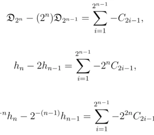
In the proof of the theorem we construct a series of projective models (Bn) ofXkn×kn Xkn independent of the functiong and Cartier divisorsDnon eachBnsuch thatgBn,gn → g ◦τ for n → ∞. We want to relate the corollary to the following result of Kolb (cf.
[Kol16a, Theorem 3.32]), which has been stated before in a similar way for different models by Zhang (cf. [Zha10, Prop. 3.3.1, 3.4.1]):
Theorem (Zhang,Kolb)
Assume thatg0, g1, g2 are functions onS(X×k◦X)such that the restriction to each canon- ical chart is of class C2. Denote by Din the Cartier divisors on Bn from above such that
1. INTRODUCTION 7
gBn,Din →gi◦τ. Then the limit of the series of local intersection numbers 1
n3 hD0,n,D1,n,D2,ni
n∈N
exists for n→ ∞ and equals Z
S(X×k◦X)
∂xf0∂yf1∂xyf2+ permutations. (ZF) By x and y we mean local coordinates in the canonical charts.
The context of this result is as follows. In [GS95] Gross and Schoen have constructed amodified diagonal cycle ∆0 on the triple productX×KX×KXof a curveX over a global fieldK, which is a 1-dimensional cycle and is homologically trivial. They define the height pairingh∆0,∆0i in the sense of Beilinson–Bloch of ∆0 with itself. Later in [Zha10] Zhang relates this number with the self intersectionωa2 of the admissibly metrised dualising sheaf ωa of X in the following shape.
ωa2 =h∆0,∆0i+ local contributions
The local contributions are (up to a factor) integrals of the form (ZF) for a special choice of the functions fi. These terms come from harmonic analysis on graphs and these been shown to be positive in [Cin11]. Assuming h∆0,∆0i ≥0 which is presently known in the case of K =C(T) this yields ωa2 >0. By [Zha93] this is in turn known to be equivalent to Bogomolov’s conjecture on the distribution of points of small height on X.
We are now confronted with two quantities. One quantity is the local height ofX×kX with respect to the DSP arithmetic divisors 0 +gi for i ∈ {0,1,2}. The other quantity is the number (ZF) occuring as a limit of local intersection numbers. In fact these two numbers coincide which is not clear neither from the existence of the limit of the intersec- tion numbers, nor from the property that g◦τ is DSP. Kolb ([Kol16a, Ex. 3.36]) gives a counterexample of a DSP arithmetic divisor onP1×kP1 where the limit of intersection numbers does indeed depend on the way the Green’s function of this divisor is approxi- mated. It was first observed by Zhang in [Zha95] that the height is independend of the approximating sequence whenever this sequence satisfies certain positivity conditions i.e., semipositivity using an important result of Kleiman [Kle66].
In fact in our situation we achieve the following result:
Corollary (Cor. 4.3.2)
The formula (ZF) computes the local height of X×kX with respect to 0 +f0◦τ,0 +f1◦ τ,0 +f2◦τ.
The main ingredient to the proof of this corollary is Theorem A. Fixi∈ {0,1,2}. It is known from algebraic geometry, that each divisorDin can be written as the difference of ample ones, sayDin=D0in−D00in. The problem is, that this decomposition is not canonical in general and one has to achieve that the sequences of Green’s functionsgBn,D0
in orgBn,D00
in
converge forn → ∞. In our work we can show that iffi satisfies some convexity condition CC, there is an ample divisor M on1 each Bn and a positive constant C ∈ N such that C·M+Din is vertically nef for all n. In fact, Mcan be chosen rather freely. The prove relies on explicit computations of intersection numbers of curves in the special fibre of Bn. Now by construction fi ◦τ =gB,M+fi◦τ −gB,M is DSP and the associated model functions gBn,M+Din converge for n→ ∞. This convergence is the essential ingredient to
1to be precise: There are mapsBn→B1for eachnandMis the pull-back of a fixed line bundle on B1.
prove the formula for the local height. From this point on the statement of the theorem follows formally. To extend the results to arbitraryC2 functions we show that every such function can be written as the difference of CC functions which is a purely analytic task.
One application of the explicit formula lies in solving partial differential equations on (X×kX)an
K. Let Y be an arbitrary projective variety of dimension d overk. Let Di+fi be DSP arithmetic divisors fori∈ {1, . . . , d}and set D0 as the trivial divisor. The rule
f0 7→λ(D+fi)i∈{0,...,d}(Y)
which assigns to each DSP Green’s function f0 for the trivial divisor the local height of Y with respect to D0+f0, . . . , Dd+fd determines a measure onYan
K , the Chambert-Loir measure, which we will denote by
c1(O(D1),k · kf1)∧. . .∧c1(O(Dd),k · kfd).
By solving partial differential equations on (X×kX)an
K we mean the following: Given a measureµ we look forf1, f2, f such that
µ=f ·c1(OX×kX,k · kf1◦τ)∧c1(OX×kX,k · kf2◦τ)
wheref, f1, f2 may be subject to constraints. In our work we focus on two kinds of partial differential equations: Monge–Amp`ere type and Poisson type differential equations. The first kind of differential equation has been investigated in [YZ10], [Liu11] and [BFJ15].
The second kind has been proposed by Shou-Wu Zhang in [Zha15]. It was observed in [Liu11] that explicit formulae for local heights can be used to solve differential equations by reducing to differential equations on real manifolds. In our case, the explicit formulae for the local height allow us to reduce our differential equations to the real Monge-Amp`ere equation and a linear elliptic equation of second order respectively.
Theorem B
2 Let f : |Γ|2 → R be a smooth function such that the support of f is contained in a canonical square S = [0,1]2 and has empty intersection with the topological boundary of S in R2. Let g: |Γ|2 → R be a smooth function. Assume that u : S → R is a smooth solution of the partial differential equation
f(∂xxg∂yyg−2(∂xyg)2) = ∂xxg∂yyu+∂yyg∂xxu−2∂xyg∂xyu
supported in the interior of S. Then u◦τ is a solution for the Poisson problem i.e., c1(O(X×kX)an
K ,k · ku◦τ)∧c1(O(X×kX)an
K ,k · kg◦τ) = f·c1(O(X×kX)an
K ,k · kg◦τ)∧c1(O(X×kX)an
K ,k · kg◦τ) holds.
Another aspect of the functions fi ◦τ is the following: Let Y be a good K-analytic space. In [CLD12] Chambert-Loir and Ducros have developed a theory of smooth differ- ential forms and currents of type (p, q) on Y. Roughly the idea is locally regarding the Berkovich space as a tropical variety and then using the differential forms from tropical geometry developed in [Lag12]. Chambert-Loir and Ducros have developed a theory of plurisubharmonic metrics on line bundles or psh for short in this context of differential forms. There is also a way of integration (n, n)-forms onn-dimensional Berkovich spaces.
If a metric can be written as the limit of psh metrics, then the say it ispsh-approximable.
If a metric is the quotient of two psh-approximable metrics, then they call itapproximable.
2On request of the reviewers the statement of Theorem B has been changed.
1. INTRODUCTION 9
For a psh approximable metrick · kon a line bundle Lof Y there is a well defined Chern- current c1(L,k · k). Moreover, products of such Chern currents can be obtained using an analogue of Bedford-Taylor theory.
Let Y be a projective variety over k. Any arithmetic divisor D+g defines a metric k · kg on O(D). Now we can compare the different notions of positivity of metrics as follows.
Theorem C
Let Y be the analytification of a projective variety of dimension d. Then
(i) If D+g is semipositive then the metric k · kg is a psh-approximable metric on O(D)an
K,
(ii) ifD1+g1, . . . , Dd+gdare semipositive then the Chambert-Loir measure associated to these DSP arithmetic divisors coincides with the measure associated to the wedge product of the Chern currents c1(O(D1),k · kgi◦τ) for i∈ {1, . . . , d}.
Point (i) is due to Chambert-Loir and Ducros in case the metrics come from modelsD where some power of O(D) is a globally generated line bundle. We generalise this result to the semipositive case using a result from [BFJ16] which in turn we had to generalise to the non-discretely valued case. Then (ii) follows from purely measure-theoretic arguments.
We turn back to the case of the self product of a curve. Now our approximation theorem implies that fi◦τ determines an approximable metric on the trivial line bundle and we can evaluate the integral
Z
(X×kX)an
f0◦τ·d0d00(f1◦τ)∧d0d00(f2◦τ) (DF) explicitly which is the integral off0against the product of the Chern currentsc1(OX×X,k·
kfi◦τ) for i ∈ {1,2}. Using the previous theorem we see that this is the local height of X×X with respect tof0◦τ, f1◦τ, andf2◦τ. Assume now thatfi is a smooth function on each canonical square for all i∈ {0,1,2}. We can show (cf. Thm. 5.4.2) that each fi ◦τ is a smooth function in the sense of [CLD12] on the dense open subsetQ of (X×kX)an which is the preimage of all topological interiors of charts|Γ|2 isomorphic to [0,1]2 underK
the retraction τ.
Theorem D (Thm. 5.5.2 (i))
We have the following explicit formula for the integral Z
Q
f0◦τ ·d0d00(f1◦τ)∧d0d00(f2◦τ) = Z
S(X×k◦X)
f0∂xxf1∂yyf2− Z
S(X×k◦X)
f0∂xyf1∂xyf2, (SP) We also show that if all fi ◦τ are smooth functions in the sense of Chambert-Loir and Ducros then this is in fact the integral over the whole analytification. The essential ingredient for the proof of our theorem is the computation of thecanonical calibration, i.e., data for the integration of (2,2)-forms coming from tropical geometry. Here the interplay with the geometry of the Berkovich space is essential: For example, the formula would not hold true ifek was not algebraically closed.
Comparing (DF) and (SP) we get a decomposition of the local height into a smooth contribution which is an integral over Q and asingular contribution, which is an integral with respect to a measure supported in the complement of Q.
The structure of this text is a follows: In Chapter 2 the necessary definitions and constructions are given. Chapter 3 is devoted to our approximation theorem: In Section
3.1 we discuss the analysis of a suitable class of functions on the geometric realisation of products of graphs. In Section 3.2 we construct the models which we will use for showing the DSP property of arithmetic divisors and investigate the structure of the special fibre.
In Section 3.7 we will show the DSP property for a class arithmetic divisors on products of curves. To illustrate the ideas of the proof we do the baby case of a curve in Section 3.6. Finally we compare our result with existing results, one due to Liu (cf. [Liu11]) and one due to Burgos, Philippon, and Sombra (cf. [BGPS14]).
Chapter 4 is devoted to applications: We prove our results on local heights ofX×kX.
Here we also give the application of our approximation theorem to differential equations of Monge-Amp`ere type and Poisson type.
Chapter 5 is devoted to the theory of smooth differential forms by [CLD12] and Monge-Amp`ere measures. Here we prove our comparison results between the smooth setting and the setting of DSP arithmetic divisors.
Acknowledgements: I would like to express my gratitude to my supervisor Klaus K¨unnemann for inspiring discussions, many of the ideas contained in this thesis, patience, and guidance during my PhD. I would also like to thank my co advisor Walter Gubler for many discussions and ideas, and for encouraging me to pursue ideas. I want to thank Johannes Kolb for explaining his thesis to me which was the starting point for my thesis.
I am very grateful to Christian Dahlhausen, Julius Hertel, Philipp Jell, Florent Martin, and Jascha Smacka for numerous inspiring discussions. I want to thank Ruben Jakob and Nikolai Nowaczyk for answering me questions to the fourth chapter. I acknowledge support from the DFG graduate school GRK 1692 Curvature, Cycles, and Cohomology in Regensburg.
Moreover, I would like to thank my parents Brigitte and Werner Vollmer for support- ing me during my studies in mathematics for the last 8 years and I want to thank my companion Magdalena K¨archer for support and consolation during the last years.
CHAPTER 2
Definitions and Constructions
2.1. Notations/Conventions
The natural numbers are assumed to contain zero. For two sets we write A ⊂ B if every element of A is contained in B. In particular, we allow equality. By an order on a set S we will mean a total order. For a subset Z ⊂ Rn we denote by convhull(Z) the convex hull of Z in Rn. A variety is an integral separated scheme of finite type over a field K. If Z ⊂ X is a closed subscheme of a scheme X then we denote by Zred the closed subscheme of X which has the unique reduced closed subscheme structure of Z.
Unless otherwise stated a divisor on a scheme will always be a Q-Cartier divisor. We write divisors additively and reserve the multiplicative notation for line bundles. Let R be a ring. By X ×RY we mean X ×SpecRY for two R-schemes X and Y. If S/R is a ring extension we denote by XS the base changeX×RSpecS. We say that a morphism ϕ: X →Y of schemes isprojective if it factors into a closed immersion X →Y ×SpecZPmZ and the projection to Y for some m ≥ 1. This kind of morphism is sometimes called H-projective. We say that a line bundle L is very ample relative to Y if there exists an immersion i: X ,→ Pm ×SpecZY such that i∗O(1) ∼= L. An immersion is an open immersion followed by a closed immersion.
LetK be a field which is complete with respect to a non-Archimedean absolute value and f : X →Y be a morphism ofK-analytic spaces in the sense of Berkovich. Then we denote by Int(X/Y) the interior of f and by∂(X/Y) the boundary.
2.2. Berkovich Analytification
We recall the definition of the analytic space associated to an admissible formal scheme as in [Ber94, §1]: Let K be a field which is complete with respect to a complete non- trivial non-Archimedean absolute value|·|. LetK◦ be the valuation ring,K◦◦the maximal ideal andKe be the residue field. Let η, s be the generic and the special points of SpecK◦ respectively. We say that a schemeXoverK◦ isvertical if the the image of the canonical map X→Spec(K◦) is the special point. By an admissible algebra we mean a K◦-algebra isomorphic to a K◦-torsion-free quotient of K◦hx1, . . . , xni by an ideal I. We denote by Spf(A) the formal spectrum of an admissible algebraA. Anadmissible formal scheme is a formalK◦-scheme which admits a locally finite cover by Spf(A) for admissibleK◦-algebras A.
The analytic space associated to Spf(A) of an admissible formal algebraAisM(A⊗K◦ K), whereM(B) is the Berkovich spectrum of an affinoid algebraB as defined in [Ber90, 1.2]. The special fibre over K◦ is defined as Spec(A⊗K◦ Ke). These definitions globalise yielding the analytification Xan and the special fibre Xs of X for an admissible formal scheme X. This construction is functorial: For a K◦-morphism ϕ: X → Y between admissible formal schemes we get a morphism ϕan: Xan → Yan between the associated
11
analytic spaces. Furthermore, there is a reduction map πX: Xan →Xs
which is surjective by [Ber90,§2.4].
Let X be a K-analytic space. A formal model of X is a proper admissible formal scheme X with a distinguished isomorphism Xan ∼= X. Let X be a separated scheme of finite type overK. In virtue of [Ber90, Thm. 3.4.1] we associate to X the analytification Xan. This construction is also functorial. So, for a separated algebraic scheme Bof finite presentation overK◦ we have two ways of associating a Berkovich analytic space with it:
First we can take the generic fibre ofBand take the associated analytic space (Bη)an. We will denote this analytic space by Ban. On the other hand we can consider the analytic space Bban associated to the completion Bb of B along the special fibre. There is always a functorial inclusion Bban ,→ Ban which is an isomorphism if B is proper (cf. [Thu07, Prop. 1.10]). We will be in the following setting repeatedly.
Assumption 2.2.1
Letk be a field which is complete with respect to a non-trivial non-Archimedean discrete absolute value. Let k◦ be the valuation ring of k and π be a uniformiser. Set b = |π|−1. Let ek be the residue field. Assume that ek is algebraically closed. Let kn be the totally ramified extension ofkof degreen. We denote byKthe completion of an algebraic closure of k, K◦ the valuation ring ofK, and by K◦◦ the maximal ideal of K◦. We consider kn as embedded intoK and equipped with the induced absolute value.
2.3. Arithmetic Divisors
We will introduce the language of arithmetic divisors on projective varieties over a non-Archimedean valued field which is partially a generalisation of the definition given in [Mor16].
We will be in the situation of Assumption 2.2.1.
Convention 2.3.1
LetB be a scheme over k◦n. Unless otherwise stated, by the generic and special fibre we mean the generic resp. special fibre over the generic and special point ofk◦n. Under abuse of notation we will denote them by Bη and Bs respectively.
Definition 2.3.2
LetX be a geometrically integral, projective variety over k.
(i) For d ∈ Q let D = qD0 be a Q-Cartier divisor on X such that D0 is an integral Cartier divisor. Then a Green’s function for D is a continuous function
g : (XK)anrsupp(D0
K)an →R
such that if (fi)i∈I are local equations for D0 on an open covering (Ui)i∈I of X, for each i∈I the function
g+qlogb|fi|2 :Ui,anKrsupp(D0K)anred→R extends to a continuous function on eachUi,an
K.
(ii) A pair of aQ-Cartier divisorD and a D-Green functiong will be called arithmetic divisor and written D+g. The set of arithmetic divisors has naturally the structure of aQ-vector space.
2.3. ARITHMETIC DIVISORS 13
(iii) Let D0 be a Z-Cartier divisor on X. Let X be a model of X over kn◦, that is a projective flat scheme overk◦n with a distinguished isomorphismX⊗kn◦kn ∼=X⊗kkn, and let D0 be a model of a Cartier divisor D0 on X, that is a Q-Cartier divisor D0 on X and an isomorphismD0|η compatible with the isomorphismX⊗kn◦kn ∼=X⊗kkn. Assume that D0 is aZ-Cartier divisor. We denote by πX: (XK)an →X⊗Ke the reduction map. For any x∈ Xan
K letf be a local equation for D around πX(x). Then themodel Green’s function gX,D0 is given by
gX,D0(x) = −logb|f(x)|2.
Clearly, the definition of model functions can be extended toQ-Cartier divisors onXand X respectively. For the rˆole of b in the definition of gX,D0 cf. Rem. 3.3.1 later on.
(iv) Letg, hbe twoD-Green’s functions. Theng−his a Green’s function for the trivial Cartier divisor and we can define the distance of g and h by
d(g, h) = sup
x∈Xan
K
|(g−h)(x)|.
The space Xan
K is compact, as X was assumed projective. Hence d attains only finite values and so defines a distance on the space of Green’s functions for D, indeed.
(v) We say that D+g issemipositive if g is the limit with respect to the distance d of model functions gXl,Dl where each Dl is a vertically nef Q-Cartier divisor on a model Xl, that is, the degree of O(Dl) restricted to any complete curve in the special fibre of Xl is non-negative.
(vi) We say that an arithmetic divisor is adifference of semipositive arithmetic divisors orDSP for short if it can be written as a difference of semipositive ones.
CHAPTER 3
The Approximation Theorem
3.1. Analysis on Products of Graphs
In this section we develop the analysis which will be used to prove our approximation theorem. Namely we will define a notion of positivity of real valued functions on the self product of the geometric realisation of a graph and will show that a large class of differentiable functions can be written as a difference of this kind of positive functions.
These positive functions functions will give rise to DSP Green’s functions for the trivial divisor. In the following let Γ be a finite graph in the sense of Def. A.4. In particular every edge of Γ has an orientation.
Definition 3.1.1
We define thevalence of Γ, denoted by val(Γ), as the maximal number of edges connected to a vertex.
Definition 3.1.2
Let Γ be a graph. Assume that Γ has no loop edges. The orientation on the edges of Γ provides us with an atlas of canonical charts on the self product |Γ|2 of the geometric realisation of Γ (cf. Appendix A) each of them isomorphic to [0,1]2. Choose coordinates x, y of [0,1]2. By dividing [0,1]2 into the standard simplices {x ≤ y} and {x ≥ y} we define the canonical two-simplices of |Γ|2.
x y
(0,1)
(1,0) (0,0)
(1,1)
{x≤y}
{x≥y}
Figure 3.1.1. A canonical chart with the canonical two-simplices
(i) The relative boundary of [0,1]2 is the topological boundary of [0,1]2 in R2. The relative boundary of |Γ|2 is the union of all relative boundaries of canonical charts. It will be denoted by relbd(|Γ|2). The relative interior is the complement of relbd(|Γ|2) in |Γ|2 and will be denoted by relint(|Γ|2).
(ii) Let Z be a closed subset of Rn for n ≥ 1. We say that a real valued function f: Z →R is of class Ck onZ if there exists an open set U ⊃Z such that f extends to a Ck(U)-function. We say that f is smooth if there exists a neighbourhood U of Z in Rn such thatf extends to a smooth function on U.
(iii) Let f:|Γ|2 →R be a continuous function. Let k ∈N∪ {∞}be a number. We say f is a Ck function on |Γ|2 if the restriction of f to every chart in the atlas associated to |Γ|2 is a Ck function on [0,1]2. Then, we say that f is Ck on the squares and denote the space of these functions by C2k(Γ2). If moreover, we demand the restriction of this
15
function to each canonical square to attain rational values at rational points then we write f ∈ C2k,Q(Γ2).
(iv) If f is aCk-function on |Γ|2 and i ∈ {1,2} we can define differential operators∂xi for i1, . . . , in ∈ {1,2} as follows. Let Z be a chart of |Γ|2 and consider f as a function on [0,1]2. Then ∂xif is the usual derivative with respect to the i-th coordinate on the relative interior of [0,1]2. This extends to a function ∂xi
1···xinf on the relative interior of
|Γ|2. Accordingly we define higher partial derivatives.
(v) Similarly we introduce the spaceC∆k(Γ2) of functions which areCk on the canonical two-simplices of |Γ|2 as the space of continuous functions on |Γ|2 whose restrictions to the canonical 2-simplices are Ck. For such functions it makes sense to define the partial derivatives on the union of the relative interiors of the canonical two simplices. If we demand that in each chart the partial derivatives in x and y direction up to the k-th order attain rational values at rational points then we writeC∆,k
Q(Γ2).
(vi) Let f: [0,1]2 → R be a function. We say that f satisfies the convexity condition CC if
(a) It is Lipschitz continuous on each square.
(b) For everyx, y ∈[0,1] and every ε >0 such that x+ε∈[0,1] and y+ 2ε∈[0,1] the inequality
g(x+ 2ε, y+ε)−g(x+ε, y)−g(x+ε, y+ε) +g(x, y)≥0 (CC1) holds. For everyx, y ∈[0,1] and everyε >0 such thatx+2ε∈[0,1] andy+ε∈[0,1]
the inequality
g(x+ε, y+ 2ε)−g(x, y+ε)−g(x+ε, y+ε) +g(x, y)≥0 (CC2) holds. For everyx, y ∈[0,1] and everyε >0 such thatx+εand y+ε lie in [0,1] we demand that
g(x+ε, y) +g(x, y+ε)−g(x, y)−g(x+ε, y+ε)≥0 (CC3) holds. We will speak of CC-functions for short for functions which satisfy the convexity condition CC.
(vii) Let f: |Γ|2 → R be a function. We say that f satisfies CC if the restriction of f to every chart of the atlas associated to Γ2 is a function which satisfies CC.
Remark 3.1.3
(i) The property of a function of beeing CC on a graph depends on the orientation of the edges of a graph. A priori it is not clear how the property of beeing CC behaves under refinement of graphs.
(ii) Not every convex function on [0,1]2 is a CC function. For example x2+xy+y2 is convex but not CC.
Definition 3.1.4
If f: |Γ|2 → R is a continuous function we can define the integral R
|Γ|2f: For every canonical chartZ ∼= [0,1]2 we defineR
Zf =R
[0,1]2f with respect to the standard Lebesgue measure of total mass one. We define R
|Γ|2f as the sum over all R
Zf for all canonical chartsZ of|Γ|2. Letf: relbd(|Γ|2)→Rbe a continuous function on the boundary. LetZ be a canonical chart of|Γ|2. Then we defineR
∂Zf as the integral off over the topological boundary of Z in R2. The space ∂Z is the union of four copies of the unit interval on which we have the standard Lebesgue measure each. We define
Z
relbd(|Γ|2)
f =X
Z
Z
∂Z
f,
3.1. ANALYSIS ON PRODUCTS OF GRAPHS 17
where the Z runs over all canonical charts of|Γ|2. Remark 3.1.5
Every CC-functionf: [0,1]2 →R satisfies
f(x, y) +f(x+ 2ε, y)−2f(x+ε, y)≥0 (3.1.1) and
f(x, y) +f(x, y+ 2ε)−2f(x, y+ε)≥0. (3.1.2) Indeed
f(x, y) +f(x+ 2ε, y+ε)−f(x+ε, y+ε)−f(x+ε, y)≥0 and
−f(x+ε, y)−f(x+ 2ε, y+ε) +f(x+ε, y+ε) +f(x+ 2ε, y)≥0
holds and adding these two inequalities we get (3.1.1) and similarly we get (3.1.2). Fur- thermore, it can be shown that the conditions (3.1.1), (3.1.2), and (CC3) jointly imply (CC1) and (CC2). However, the condition CC has the advantage that it can be checked
”locally”1 on each square, which will be useful in the proof of Prop. 3.1.13.
For later applications we are interested in functions on the self-product of a graph which can be written as differences of CC-functions. It can be shown that C2-functions on a closed subset of Rn can be written as a difference of convex functions. In analogy to this result we will show that C22,Q-functions on the self product of a graph after a suitable subdivision of the graph can be written as the difference of two CC functions.
In the remainder of the section we will prove the following theorem which is the crucial ingredient in our approximation theorem. The theorem is divided in two parts: The first claims that every C2 function on the self product of the S-subdivision in the sense of Def. A.9 of a finite graph can be written as a difference of CC-functions. Moreover, the second allows non-differentiability along the diagonals. Although the first claim follows from the second and the ideas of the proof are essentially the same, the second proof is much more technical due to the techniques of smoothening which are applied.
In the sequel we will assume Γ is a finite graph such that (i) Γ has more than one vertex and at least one edge,
(ii) Γ has no double edges that is, for two vertices v1, v2 there is at most one edge linking v1 and v2,
(iii) Γ has no loop edges.
Theorem 3.1.6
Assume that Γ be the S-subdivision of a finite graph. Let f: |Γ|2 → R be a continuous function.
(i) If f ∈ C22(Γ2) then it is the difference of two CC-functions g, h in C22(Γ2). If furthermore f ∈C22,Q(Γ2) then g and h can be chosen in C22,Q(Γ2),
(ii) if f ∈ C∆4(Γ2) then it is the difference of two CC-functions in C∆2(Γ2). If fur- thermore f ∈C∆,4
Q(Γ2) then g and h can be chosen in C∆,2
Q(Γ2).
Proof. We define an auxillary functiona: |Γ|2 →R. Let x, y be local coordinates in one of the canonical charts of Γ. Then we define
a(x, y) =x2−xy+y2. (3.1.3)
1i.e. in an appropriate G-topology on |Γ|2
In Figure 3.1.2 we have depicted all eight possible ways how the canonical charts of |Γ|2 can intersect a fixed chart, which is filled in grey. The arrows at the diagonals indicate the diagonal from (0,0) to (1,1) in the canonical charts. Then it is easy to see that a is well-defined. This special structure of the canonical charts of |Γ|2 is due to to the fact that Γ is the S-subdivision of some graph (cf. Rem. A.11 and A.8).
Figure 3.1.2. All eight ways how charts in an S-subdivision can intersect.
The arrow is the diagonal from (0,0) to (1,1) in each canonical chart
Let x, y be local coordinates in a canonical chart and ε > 0. Then we have the following equalities.
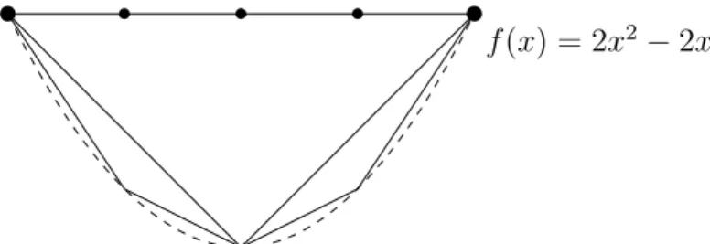
a(x+ 2ε, y+ε)−a(x+ε, y)−a(x+ε, y+ε) +a(x, y) =ε2, (3.1.4) a(x+ε, y+ 2ε)−a(x, y+ε)−a(x+ε, y+ε) +a(x, y) =ε2, (3.1.5) a(x+ε, y) +a(x, y+ε)−a(x, y)−a(x+ε, y+ε) =ε2. (3.1.6) This shows thatais a CC function. Accordingly, whenever the failure of a function to be CC is at least of quadratic order forε→0, we can use positive multiples of a (which are again CC) to make it CC.
We begin with the proof of (i): We restrict f and a to a canonical square which we identify with [0,1]2 and introduce coordinates x, y. We will now show that there is a real constantM ≥0 such thatM·a+f satisfies CC. As|Γ|2 can be covered by finitely many canonical charts we can choose M large enough that this holds for every square. Then M a is CC and M a+f is CC hence f =M a+f−M a is difference of two CC functions and we have shown our claim.
Note the following lemma:
Lemma 3.1.7
Let f: [0, b] → R be a continuous function and let f be twice continuously differentiable on (0, b). Then we have the estimate
1
2[f(0) +f(b)]−f(b/2)
≤ 1
4b2kf00k∞
where k · k∞ is the sup-norm on C0([0,1]).
Proof. We compute
f(0) +f(b)−2f(b/2) (b/2)2
=
f0(ζ)−f0(ξ) b/2
for suitable ζ ∈(b/2, b) and ξ ∈(0, b/2) by the mean value theorem. Then
f0(ζ)−f0(ξ) b/2
≤
f0(ζ)−f0(ξ)
1
2(ξ−ζ)
3.1. ANALYSIS ON PRODUCTS OF GRAPHS 19
which equals
2|f00(η)|
for a suitable η∈(0, b) again by the mean value theorem, hence the claim.
Applying Lemma 3.1.7 to the restriction of f to the lines convhull({(x+ε, y),(x+ ε, y+ε)}) and convhull({(x+ 2ε, y+ε),(x, y)}) respectively we conclude
−f(x+ε, y)−f(x+ε, y+ε)≥ −Cε2 −2f(x+ε, y+ε 2) and
f(x+ 2ε, y+ε)−f(x+ε, y)−f(x+ε, y+ε) +f(x, y)
≥ −Cε2 −2·f(x+ε, y+ ε
2) +f(x+ 2ε, y+ε) +f(x, y)≥ −Cε2−5ε2·C
for C = 14kf00k∞. So (3.1.4) shows that we can choose M >0 such that M a+f satisfies (CC1). The argument for (CC2) follows by symmetry as the condition (CC2) is the same as (CC1) withx andy interchanged. Likewise we see that there exists a C >0 such that
−f(x, y)−f(x+ε, y+ε)≥ −Cε2−2f(x+ ε
2, y+ ε 2).
IncreasingC we get
f(x+ε, y) +f(x, y+ε)−2f(x+ ε
2, y +ε
2)≥ −Cε2 and finally
f(x+ε, y) +f(x, y+ε)−f(x, y)−f(x+ε, y+ε)≥ −2Cε2.
Accordingly we can increase M to achieve (CC3) for M a+f. Now the proof of (i) is complete.
For the proof of (ii) we define another auxilliary function b defined in canonical coor- dinatesx, y by
b(x, y) = |x−y|.
We have the equalities
0 =b(x+ 2ε, y+ε)−b(x+ε, y)−b(x+ε, y+ε) +b(x, y) and
0 =b(x+ε, y+ 2ε)−b(x, y+ε)−b(x+ε, y+ε) +b(x, y) and
b(x+ε, y) +b(x, y+ε)−b(x, y)−b(x+ε, y+ε) =
(0 for |x−y|> ε 2ε−2|x−y| for |x−y| ≤ε.
(3.1.7) Which in particular shows, thatb is a CC-function.
Definition 3.1.8
Let f: U → R be a function on an open subset of Rn for some n ≥ 1. Let v ∈ Rn be a vector. We will use the following notation for one-sided partial derivatives
∂v+f(x) = lim
t&0
f(x+tv)−f(x)
|t| , ∂v−f(x) = lim
t&0
f(x−tv)−f(x)
|t| .
and similarly define higher one-sided derivatives.
The following lemma will be used for the regularisation of functions on [0,1]2 with singularities along the diagonal with functions which are differences of CC functions.
Lemma 3.1.9
Let g: [0,1]2 →R be a continuous function which is of class C2 on the sets {x ≥y} and {x≤y} respectively. We define:
kg(x, y) =
1
2(y−x)∂(1,−1)+ g(12(x+y),12(x+y)) if x≤y, y 6= 0, x6= 1
1
2(x−y)∂(1,−1)− g(12(x+y),12(x+y)) if x > y, x6= 0, y 6= 1
0 otherwise.
Then
(i) The function g+kg is of class C1 on [0,1]2.
(ii) There exists an M > 0 such that kg+M(a+b) is CC on [0,1]2. Proof.
(i) The functiong+kgisC1at all points except possibly at the diagonal. By construction
∂(1,−1)+ kg(z, z) = lim
t&0
2t∂−(1,−1)g(z, z)−0
2t =∂(1,−1)− g(z, z) and
∂(1,−1)− kg(z, z) = lim
t&0
2t∂+(1,−1)g(z, z)−0
2t =∂(1,−1)+ g(z, z) hold for all z ∈[0,1]. So we have the equality
∂(1,−1)+ (g +kg) = ∂(1,−1)+ g+∂(1,−1)− g =∂(1,−1)− g+∂(1,−1)+ g =∂(1,−1)− (g+kg).
The two-sided partial derivatives ∂(−1,1) of kg and g exist everywhere in [0,1]2 and are continuous. Now the gradient of g+kg on the triangle {x≥y} ⊂[0,1]2 agrees with the gradient on the triangle {x≤y}. As we assumed thatg is differentiable on each of these triangles, this implies, thatg+kg is differentiable on [0,1]2 and hence the first part of the lemma.
(ii) AsgisC2 on the closed subsets{x≥y}and{x≤y}of [0,1]2 we can chooseM >0 such that M ·a+kg satisfies (CC1), (CC2), and (CC3) whenever all points appearing in these inequalities are contained in either one of the subsets {x ≤ y} or {x ≥ y} of [0,1]2. This can be seen by extending the restriction of the function kg to a C2 function on the upper (resp. lower triangle) to the whole square and applying the first part of the theorem. We see that all points in the inequality (CC1) are contained in the same two-simplex of [0,1]2 if and only if|x−y| ≥ ε. Indeed, assume by symmetry that y ≥x holds. Then for every ε >0
y ≥x∧y ≥x+ε∧y+ε≥ε+ 2ε∧y+ε≥x+ε ⇔y≥x+ε holds.
Let ε >0 be a positive number. Now choose x, y with |x−y| ≤ε to treat the cases where possibly not all coordinates in the inequalities (CC1), (CC2), and (CC3) lie in the same triangle of [0,1]2. By symmetry assume y ≥x. Then
|kg(x, y)−kg(x+ε, y+ε)|
= 1
2|x−y| ·
∂(1,−1)+ g(1
2(x+y),1
2(x+y))−∂(1,−1)+ g(1
2(x+y) +ε,1
2(x+y) +ε)
≤ε2C,
3.1. ANALYSIS ON PRODUCTS OF GRAPHS 21
whereConly depends on the Lipschitz constants of the first partial derivatives of g which are finite by the mean value theorem. Now if y≥x and |x−y| ≤ε then y+ε≤x+ 2ε and y≤x+ε. Hence
|kg(x+ε, y)−kg(x+ 2ε, y+ε)|= 1
2|x−y| ·
∂(1,−1)− g(1
2(x+y+ε),1
2(x+y+ε))
−∂(1,−1)− g(1
2(x+y+ 3ε) +ε,1
2(x+y+ 3ε))
≤ε2C,
holds for a constant C only depending on g again by the Lipschitz continuity of the first partial derivatives. So after possibly enlargingM we can arrange that (CC1) and (CC2) are satisfied forM ·a+kg on the whole of [0,1]2 for all ε >0.
It remains to show that we can achieve (CC3). Note that (CC3) is satisfied forM·a+kg whenever |x−y| ≥ε. So let x, y be such that|x−y| ≤ε. We can assume that x≤y by symmetry. Then the point (x, y) is contained in the closed segment L⊂[0,1]2 from
(1
2(x+y)−ε
| {z }
=:z1
,1
2(x+y) +ε
| {z }
=:z2
) to
(1
2(x+y)
| {z }
=:z01
,1
2(x+y)
| {z }
=:z20
).
We define kN0 (z, w) =N(a(z, w) +b(z, w)) +kg(z, w) for any numberN ≥0 and set kN(z, w) := k0N(z+ε, w) +kN0 (z, w+ε)−k0N(z, w)−kN0 (z+ε, w+ε)
for (z, w)∈[0,1]2 such thatz+ε ≤1 andw+ε ≤1. The restriction of kN toL is affine for any N ≥ 0 as ε is fixed. So to check kN(x, y) ≥ 0 it suffices to check kN(z1, z2) ≥ 0 and kN(z10, z20)≥0. Note that forN =M we have kN(z1, z2) ≥0. By (3.1.6) and (3.1.7) we have the following equality.
kN(z10, z20) = 2N ε+N ε2+ ε
2·∂−(1,−1)g(z10 + ε
2, z20 + ε 2) + ε
2·∂(1,−1)+ g(z10 + ε
2, z20 +ε 2) As the restrictions of the derivatives to the diagonal are bounded functions we may enlarge N such that kN(z10, z20)≥0 for all εand we are done. Enlarging M such that M ≥N, we are finished with the proof of the lemma.
Lemma 3.1.10
Assume that the functiong: [0,1]2 →R isC1 on[0,1]2 andC4 on the closed sets{x≥y}
and {x≤y}. Then we define kg2(x, y) =
(1
8(x−y)2∂(1,−1)2,+ g(12(x+y),12(x+y)) for x≤y
1
8(x−y)2∂(1,−1)2,− g(12(x+y),12(x+y)) for x > y Then:
(i) The function g+kg2(x, y) is C2 on [0,1]2,
(ii) there is an M > 0 such that M ·(a+b) +kg2 is CC.
Proof.
(i) We define functions on [0,1]2 as follows.
k+(x, y) = 1
8(x−y)2∂(1,−1)2,+ g(1
2(x+y),1
2(x+y)), k−(x, y) = 1
8(x−y)2∂(1,−1)2,− g(1
2(x+y),1
2(x+y)).
Ask+andk−are products ofC2-functions on [0,1]2 they are againC2-functions on [0,1]2. In particular k2g is a C2 function on the sets {x ≤ y} and {x≥ y} respectively. For any z ∈[0,1] we have the equality
∂(1,−1)+ kg2(z, z) = ∂(1,−1)+ k+(z, z) = lim
t&0
1 t
1
84t2∂(1,−1)2,− g(z, z)
= 0 and accordingly
∂(1,−1)− kg2(z, z) = 0.
We compute the second single-sided derivatives of kg2 at the diagonal. We do this by computing the two-sided derivative of k+ and k− respectively using difference quotients for the second derivatives. We have
∂(1,−1)2,+ k2g(z, z) = lim
t&0
1
t2 k−(z+t, z−t)−2k−(z, z) +k−(z−t, z +t)
= limt&0
1 t2
1
84t2∂(1,−1)2,− g(z, z)−0 + 1
84t2∂(1,−1)2,− g(z, z)
=∂(1,−1)2,− g(z, z) and likewise
∂(1,−1)2,− kg2(z, z) =∂(1,−1)2,+ g(z, z).
Hence
∂(1,−1)+ (g+k2g) =∂(1,−1)+ g,
∂(1,−1)− (g+k2g) =∂(1,−1)− g,
∂(1,−1)2,+ (g+k2g) =∂(1,−1)2,+ g+∂(1,−1)2,− g,
∂(1,−1)2,− (g+k2g) =∂(1,−1)2,− g+∂(1,−1)2,+ g.
at (z, z) forz ∈[0,1]. We conclude that g+kg2 is C2 on [0,1]2. (ii) We have the estimate
|k2g(z, w)| ≤C|z−w|2 (3.1.8)
for all (z, w)∈[0,1]2and a real constantC > 0 only depending ongusing the boundedness of the partial derivatives and the definition of kg2. We can find anM such that M a+kg2 is CC: Choose (x, y) ∈ [0,1]2 and ε > 0. As k2g is C2 on the two-simplices we find an M > 0 such that M a+k2g satisfies (CC1), (CC2), and (CC3) whenever |x−y| ≥2ε. If
|z−w| ≤2ε then by 3.1.8 we have
|kg2(z, w)| ≤Cε2 for some biggerC. So we conclude
|k2g(x, y)−kg2(x+ε, y)−k2g(x+ε, y+ε) +k2g(x+ 2ε, y+ε)| ≤4Cε2,
|k2g(x, y)−kg2(x, y+ε)−k2g(x+ε, y+ε) +k2g(x+ε, y+ 2ε)| ≤4Cε2,
|k2g(x+ε, y) +k2g(x, y+ε)−k2g(x, y)−kg2(x+ε, y+ε)| ≤4Cε2.