Research Collection
Doctoral Thesis
Applications of Deep Learning for Sequential Data: Music, Human Activity and Language
Author(s):
Brunner, Gino Publication Date:
2020
Permanent Link:
https://doi.org/10.3929/ethz-b-000450816
Rights / License:
In Copyright - Non-Commercial Use Permitted
This page was generated automatically upon download from the ETH Zurich Research Collection. For more information please consult the Terms of use.
ETH Library
Applications of Deep Learning for Sequential Data:
Music, Human Activity and Language
A thesis submitted to attain the degree of DOCTOR OF SCIENCES
(Dr. sc. ETH Zurich)
presented by GINO BRUNNER
MSc in Eletrical Engineering, ETH Zurich, Switzerland born on 09.07.1990
citizen of Hochdorf LU
accepted on the recommendation of Prof. Dr. Roger Wattenhofer, examiner Prof. Dr. Thomas Hofmann, co-examiner
2020
Copyright © 2020 by Gino Brunner
Series in Distributed Computing, Volume 34 TIK-Schriftenreihe-Nr. 186
Edited by Roger Wattenhofer
This thesis presents applications of deep learning to three domains of se- quential data; music, human activity recognition and natural language un- derstanding.
In part one, we present work on automatic music generation and musi- cal genre transfer. We show how a model based on two hierarchical LSTMs learns an important concept from music theory. We introduce a VAE model that leverages a novel representation of symbolic music to generate music, create interpolations and mixtures of songs, and even perform genre trans- fer. We then focus exclusively on genre transfer. To that end we employ a model based on CycleGAN to perform genre transfer solely based on note pitches. We further discuss several extensions to this model as well as a sim- ple content retention metric backed by a user study.
In part two we move away from music and instead investigate how in- ertial sensor data from smartwatches can be leveraged by neural networks to perform activity recognition for strength exercises and swimming. In ad- dition to activity recognition we also tackle repetition counting as well as swimming lane counting. For both tasks we collect large datasets using off- the-shelf smartwatches; in total our datasets features almost 100 participants.
We find that sports activity recognition can be done with high accuracy by neural networks. Remarkably, the neural network approaches require little fine-tuning and generalize very well across athletes. We also saw how wear- ing a second smartwatch on the ankle can help with certain exercises, but is in general not absolutely necessary. We introduce a constrained data collec- tion approach where participants are prompted to perform the next repetition by the smartwatch. This allows to collect more and cleaner data, as well as automate some of the labelling. We verify the ability of models trained on constrained data to generalize to unconstrained settings; such a constrained
III
data collection setting could help with crowd-sourced (unsupervised) data collection. In terms of swimming style recognition, we achieve strong results that are good enough for the use in semi-professional swimming training.
In part three shift gears for the last time and arrive at the third sequential data domain; natural language. In particular, we investigate the inner work- ings of neural networks trained on natural language tasks. We find that the properties of the latent space of character-based sequence-to-sequence mod- els can be manipulated by adding decoders that solve auxiliary language tasks. For instance, adding a POS tagging decoder causes sentences with different syntactic structures to be well separated in the latent space. Inter- estingly, models that have such a disentangled latent space also perform bet- ter in interpolation and latent vector algebra tasks. We then transition from our RNN-based models to the state-of-the-art transformer architecture, and in particular, decoder-only transformers like BERT. In transformers, input tokens aggregate context as they pass through the model, hence the name contextualized word embeddings. We challenge and verify common assump- tions underlying work trying to understand transformers by interpreting the learned self-attention distributions. We find that the tokens remain largely identifiable as they pass through the model, which gives some support to work that relates hidden tokens to input words. However, at the same time, the information is heavily mixed as tokens aggregate context, and the origi- nal input token is often not the largest contributor as measured by gradient attribution. This indicates that BERT somehow keeps track of token identity.
Overall, we caution against the direct interpretation of self-attention distri- butions and suggest more principled methods such as gradient attribution.
In dieser Arbeit werden drei Anwendungsbereiche von Deep Learning für sequentielle Daten vorgestellt: Musik, menschlicher Aktivitäten und natürli- che Sprache.
Im ersten Teil präsentieren wir Arbeiten zur automatischen Musikgene- rierung und zum Transfer zwischen Musikgenres. Wir zeigen, wie ein Mo- dell, das auf zwei hierarchischen LSTMs basiert, ein wichtiges Konzept aus der Musiktheorie lernt. Wir stellen ein VAE-Modell vor, das eine neuartige Darstellung symbolischer Musik nutzt, um Musik zu erzeugen, Interpola- tionen und Mischungen von Liedern zu generieren und sogar Genretrans- fers durchzuführen. Anschliessend konzentrieren wir uns ausschließlich auf Genretransfer; zu diesem Zweck verwenden wir ein auf CycleGAN basie- rendes Modell, um den Genretransfer ausschließlich auf der Grundlage von Tonhöhen durchzuführen. Darüber hinaus diskutieren wir verschiedene Er- weiterungen dieses Modells sowie eine einfache Inhaltserhaltungsmetrik, die durch eine Benutzerstudie evaluiert wird.
Im zweiten Teil wenden wir uns von der Musik ab und untersuchen statt- dessen, wie Sensordaten von Smartwatches von neuronalen Netzen genutzt werden können, um Aktivitätserkennung für Kraftübungen und Schwim- men durchzuführen. Neben der Aktivitätserkennung befassen wir uns auch mit der Zählung von Wiederholungen und geschwommenen Längen. Für beide Aufgaben sammeln wir große Datensätze mit handelsüblichen Smart- watches; insgesamt enthalten unsere Datensätze fast 100 Teilnehmer. Wir stel- len fest, dass die Erkennung von Sportaktivitäten mit hoher Genauigkeit durch neuronale Netze erfolgen kann. Bemerkenswert ist, dass die neurona- len Netze nur wenig Feinabstimmung erfordern und sehr gut über die Ath- leten hinweg verallgemeinern können. Wir haben auch gesehen, wie das Tra- gen einer zweiten Smartwatch am Knöchel bei bestimmten Übungen helfen
V
kann, aber im Allgemeinen nicht unbedingt notwendig ist. Wir führen einen eingeschränkten Datenerfassungsansatz ein, bei dem die Teilnehmer durch die Smartwatch aufgefordert werden, die nächste Wiederholung durchzu- führen. Dies ermöglicht es, mehr und sauberere Daten zu sammeln sowie einen Teil der Datenannotation zu automatisieren. Wir verifizieren, dass Mo- delle, die mit eingeschränkten Daten trainiert wurden, auf uneingeschränkte Daten verallgemeinern; eine solche eingeschränkte Datenerfassungsart könn- te bei der (unbeaufsichtigten) Sammlung von Daten durch crowd-sourcing helfen. In Bezug auf die Erkennung des Schwimmstils erzielen wir hohe Ge- naugkeiten, die gut genug für den Einsatz im semiprofessionellen Schwimm- training sind.
In Teil drei gelangen wir zum letzten Anwendungsbereich von sequenti- ellen Daten; natürliche Sprache. Insbesondere untersuchen wir das Innenle- ben von neuronalen Netzen, die auf Sprachdaten trainiert werden. Wir stel- len fest, dass die Eigenschaften der gelernten Repräsentationen von buch- stabenbasierten sequence-to-sequence Modellen durch das Hinzufügen von Decodern, die Hilfsaufgaben lösen, manipuliert werden können. Beispiels- weise bewirkt das Hinzufügen eines POS-Tagging-Decoders, dass Sätze mit unterschiedlichen syntaktischen Strukturen im Latent Space gut voneinander getrennt werden. Interessanterweise sind Modelle, die einen derart separier- ten Latent Space aufweisen, auch für Interpolationen und Vektoralgebra im Latent Space besser geeignet. Wir gehen dann von RNN-basierten Modellen zur Transformerarchitektur, und insbesondere BERT, über. In Transformern aggregieren Input-Tokens den Kontext während sie das Modell durchlaufen;
daher der Namecontextualized word embeddings. Wir hinterfragen und veri- fizieren allgemeine Annahmen, die vielen wissenshaftlichen Arbeiten zum Verständnis von Transformers zugrunde liegen, welche versuchen die gelern- ten Self-Attention Verteilungen zu interpretieren. Wir stellen fest, dass die To- kens beim Durchlaufen des Modells weitgehend identifizierbar bleiben, was eine gewisse Basis für die Annahmen von Arbeiten darstellt, welche Hidden Tokens mit Input Tokens gleichsetzen. Gleichzeitig werden die Input-Tokens jedoch stark vermischt, und das ursprüngliche Input-Token ist, gemäss Gra- dient Attribution, oft nicht der Hauptbestandteil der entsprechenden Hid- den Tokens. Dies deutet darauf hin, dass BERT irgendwie die Identität der Tokens beibehält. Insgesamt warnen wir vor der direkten Interpretation von Self-Attention Verteilungen und schlagen prinzipiellere Methoden wie die Gradient Attribution vor.
During my PhD I had the privilege to be surrounded by great people that helped me along on the way. First of all, I want to thank my supervisor Roger Wattenhofer for the opportunity to spend a good part of my life in his group, for the easy-going collaboration, and for his continued believe in me. Next, I want to thank Thomas Hofmann for taking the time to read this thesis; I am truly honored to have him as my co-referee.
Being a member of DISCO was a great experience, mainly thanks to all my amazing colleagues. In the following I will thank everyone in more or less chronological order of when I met them: Beat Futterknecht, for know- ing how everything works. Philipp Brandes, for transferring the duty of first coffee officer to me. Klaus Förster, for introducing me to the hidden secrets behind truly excellent cakes. Ladislas de Naurois, for starting out on the deep learning journey with me. Benny Gächter, for setting up dozens of VMs for me. Pascal Bissig, for bringing me into this, and for welcoming me to the dark side. Michael “King” König for redefining what it means to come in late. Thomas Ulrich, for being my first office mate. Friederike Brütsch, for the sweets. Sebastian Brandt, for being an inspiration in table soccer. Go- erg Bachmeier, for all the laughs and cakes. Conrad Burchert, for sparing me even more talks about bitcoin. Julian Steger, for leaving me his shiny Macbook. Stefan Schindler, for teaching me the importance of hovercrafts.
Manuel Eichelberger, for always going “härter!”. Aryaz Eghbali, for the Ira- nian sweets. Pankaj Khanchandani, for all the hilarious noises during table soccer. Yuyi Wang, for his help with my first-ever paper. Darya Melnyk, for her patience with our students. Simon Tanner for the (snowshoe) hikes and the nightly paper writing that turned out to be for nothing. Susann Arregh- ini, for meeting all my questions with a smile on her face. Oliver Richter, for his inspiring work attitude and for teaching me about reinforcement learn-
VII
ing. Jakub Silwinski for keeping King’s legacy alive. András Papp for en- lightening me about gulyás. Zeta Avarikioti, for having the most amazing rooftop terrace. Tejaswi Nadahalli, for being my Aeropress brother. Roland Schmid, for the free and delicious food-sharing lunches. Damian Pascual, for rekindling my motivation and making every day more fun. Ye Wang, for dis- infecting Roger’s office. Zhao Meng, for being amazed that I could correctly pronounce his name. Lukas Faber, for bringing fresh competition into table soccer, and for the feedback on my thesis. Henri Devillez, for his wisdom on competitive coding. Béni Egressy, simply for being a fun guy to be around.
I also want to thank my family and friends for making sure I still take time to enjoy life. Finally, my biggest thanks goes to my wife Yimmy, who has stayed strong and supportive throughout the ups, and many downs, which I have experienced during my PhD. Truly could not have done it without you!
Collaborations and Contributions
This dissertation is the result of years of work at the distributed comput- ing group, during which I have collaborated with several colleagues. Here I would like to thank all of my collaborators for their contributions and all the fruitful and interesting discussions. For each chapter of this dissertation I list the contributors in alphabetical order. All of the work in this thesis is joint work with my supervisor Roger Wattenhofer.
Chapter 3is based on the publicationJamBot: Music Theory Aware Chord Based Generation of Polyphonic Music with LSTMs[28]. Co-authors are Yuyi Wang and Jonas Wiesendanger.
Chapter 4is based on the publicationMIDI-VAE: Modeling Dynamics and In- strumentation of Music with Applications to Style Transfer[23]. Co-authors are Andres Konrad and Yuyi Wang.
Chapter 5is based on the publicationSymbolic Music Genre Transfer with Cy- cleGAN[29]. Co-authors are Sumu Zhao and Yuyi Wang.
Chapter 6is based on the publicationNeural Symbolic Music Genre Transfer Insights[26]. Co-authors are Mazda Moayeri, Oliver Richter and Chi Zhang.
Chapter 8is based on the publicationRecognition and Repetition Counting for Complex Physical Exercises with Deep Learning[130]. Co-authors are Andrea Soro and Simon Tanner.
Chapter 9 is based on the publication Swimming Style Recognition and Lap Counting Using a Smartwatch[25]. Co-authors are Darya Melnyk and Birkir Sigfusson.
Chapter 11is based on the publicationDisentangling the Latent Space of (Vari- ational) Autoencoders for NLP[27]. Co-authors are Yuyi Wang and Michael Weigelt.
Chapter 12is based on the publicationOn Identifiability in Transformers[24].
Co-authors are Massimiliano Ciaramita, Yang Liu, Damian Pascual and Oliver Richter.
1 Introduction 1
1.1 Music Generation and Genre Transfer . . . 2
1.2 Human Activity Recognition in Sports . . . 4
1.3 Understanding Neural Networks for NLP . . . 5
I Automatic Music Generation and Genre Transfer 7 2 Related Work and Background 9 2.1 Automatic Music Generation . . . 9
2.2 Style and Domain Transfer . . . 10
2.3 Music Theory Primer . . . 11
2.4 Symbolic Music and MIDI . . . 12
3 JamBot: Automatic Composition of Music Using Hierarchical Re- current Neural Networks 15 3.1 Dataset . . . 16
3.2 Model Architecture . . . 17
3.3 Results . . . 24
3.4 Conclusion and Future Work . . . 26
4 MIDI-VAE: Modeling Dynamics and Instrumentation of Music with Applications to Style Transfer 28 4.1 Model Architecture . . . 29
4.2 Implementation . . . 32
4.3 Experimental Results . . . 35
X
4.4 Conclusion . . . 39
5 Explicit Music Genre Transfer with CycleGAN 41 5.1 Model Architecture . . . 42
5.2 Dataset and Preprocessing . . . 44
5.3 Architecture Parameters and Training . . . 45
5.4 Experimental Results . . . 46
5.5 Conclusion . . . 53
6 Content Retention Metric for Genre Transfer And Other Insights 55 6.1 Methodology . . . 55
6.2 Experiments and Results . . . 57
6.3 Conclusion . . . 61
II Activity Recognition in Sports 62 7 Related Work 64 7.1 HAR in Strength Training . . . 65
7.2 HAR for Swimming . . . 67
8 Recognition and Repetition Counting for Complex Physical Exer- cises 68 8.1 Data . . . 70
8.2 Methods . . . 75
8.3 Results . . . 81
8.4 Conclusion . . . 90
9 Swimming Style Recognition and Lap Counting 91 9.1 Data . . . 93
9.2 Methods . . . 97
9.3 Results . . . 101
9.4 Conclusion . . . 105
III Understanding Neural Networks for NLP 106 10 Related Work 107 10.1 Neural Multi-Task Language Models . . . 108
10.2 Token Identity in Transformers . . . 109
11 NLP Multitasking: Analyzing the Latent Space of Multi-Task Lan-
guage Models 111
11.1 Model and Data . . . 112
11.2 Results . . . 115
11.3 Conclusion and Future Work . . . 120
12 Token Identifiability in Transformers 121 12.1 Background . . . 122
12.2 Token Identifiability . . . 123
12.3 Attribution Analysis to Identify Context Contribution . . . 129
12.4 Results for Other Datasets . . . 134
12.5 Conclusion . . . 139
13 Conclusion 140
Introduction 1
“Verdammt, I should have discovered the general theory of deep learning instead... Geoff Hinton already has more citations than me and he is not even dead yet!”
— Not Albert Einstein Every once in a while a new technology comes along that has the poten- tial to completely transform our lives. Think fire, the wheel, airplanes and the Internet. Now, I am not saying that deep learning will be able to com- pete with good old firemaking in terms of overall impact, nor that, when all is said and done, its legacy will necessarily be an equally positive one (after all, what beats not having to eat raw chicken?). However, no matter whether deep learning will manage to live up to the hype, or whether it will soon be superseded by something better in the quest for general artificial intelligence, it is definitely a fascinating technology that arguably deserves all the atten- tion it has been getting. Deep learning certainly had a captivating effect on me, and I have thus devoted the past four years of my (work) life to it. I am still fascinated by the the depth of the topic; from its roots in classical statistics and machine learning to all the amazing novel applications that let us solve problems that were thought out of reach not long ago. There has been great progress in fundamental research in deep learning, and a continued effort is
1
necessary to bring these advances to a wide range of existing and novel appli- cation domains. It is there, at the intersection between fundamental research and application, where my research has mostly taken place. This disserta- tion will take the reader on a tour through interesting applications of deep learning focused on sequential data (computer vision was too mainstream).
Sequential data is hugely important and ubiquitous in our daily lifes; from written and spoken language over video to sensor data. While research in these areas has traditionally been quite disjoint, each following its own sets of methods and developing separate theories, machine and deep learning have brought these domains somewhat closer together. For instance, a sin- gle neural network architecture (such as a recurrent neural network) can be applied across all of these domains, and since neural networks alleviate the need for manual feature engineering, domain knowledge has become less important as well (again, for better or worse). During my research I found it very appealing that many different problem domains can be approached with essentially the same set of methods. In particular, this thesis is split into three main parts, where each part deals with a different domain of se- quential data: In part one, we will investigate how we can leverage neural networks to compose music and change the style of a music piece. We also try to gain a better understanding of the inner workings of our models by analyzing learned embeddings and latent spaces. In part two, we will see how deep learning can be applied to raw sensor data collected from smart- watches to track workouts in the gym and swimming pool. Finally, the main focus of part three is on gaining a better understanding of the inner workings of neural networks for natural language processing.
1.1 Music Generation and Genre Transfer
Music has something magical about it; it is like a universal language that uni- fies humanity and has the power to touch (almost) everyone. It is also very tightly associated with creativity, a trait that we think of as typically human.
While attempts have been made at using computers to automatically com- pose music for decades, the success has been limited (how many AI artists do you currently listen to?). However, the success of deep learning has in- spired us, and made us believe that maybe with this new tool we can finally teach computers to be truly creative. Especially deep generative models that attempt to uncover the underlying data generating distribution have shown promise in creative tasks, from joke generation to music composition. The combination of creativity and machine learning is immensely fascinating to me, and I devoted a considerable amount of time to it. Hence, the first part of
this dissertation presents contributions to the field of automatic music com- position and music genre transfer.
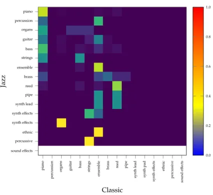
In particular, in Chapter 3 we introduce JamBot, a model that uses hier- archical recurrent neural networks (RNN) to generate music. The structure of JamBot is inspired by how humans compose music; composers first think about the long-range structures of the music piece before filling in the indi- vidual notes. Apart from being able to generate music, the most remarkable feature of JamBot are the chord embeddings that it learned: When visualized in two dimensions, the learned embeddings almost perfectly form the circle of fifths, an important tool from music theory. While JamBot can generate music, it is not per-se a generative model, and sampling new music from it is somewhat awkward since it requires a seed input to start generation.
Thus, in Chapter 4 we introduce MIDI-VAE, a model that still uses RNNs, but arranges them in a variational autoencoder (VAE) setup. The main ad- vantage of this is that MIDI-VAE learns a joint distribution over the data and latent variables, and we can then generate new examples by sampling from the latent space. MIDI-VAE also uses a more sophisticated music represen- tation; whereas JamBot only considers note pitches, MIDI-VAE can model instrumentation, velocity (loudness) and note durations as well. Another difference to JamBot is the existence of an explicit latent space which can be used to manipulate data in interesting ways; for example to interpolate be- tween music pieces to generate medleys, or even to mix multiple songs into one. Finally, by attaching a music genre classifier to the latent space we man- age to use MIDI-VAE for musical genre transfer, e.g., to transcribe a music piece from Jazz to Classic. One limitation of MIDI-VAE for genre transfer is that it mainly adapts the instrumentation, but does not change the note pitches and velocities much. Therefore, in Chapter 5 we investigate whether a music genre transfer based solely on note pitches is even feasible. To that end we use an entirely different architecture: Two generative adversarial net- works (GAN) arranged in a cycle. This architecture is generally referred to as CycleGAN and was introduced for image domain transfer [160] (think transforming a picture of a summer landscape into a winter landscape, or a painting into a photograph). Thus, in contrast to MIDI-VAE, the genre trans- fer objective is the main objective of the model, as opposed to being simply an auxiliary objective to shape the latent space. We find that with some effort, CycleGAN can be adapted to perform music genre transfer based solely on note pitches, and it does so more convincingly than MIDI-VAE. GAN train- ing is known to be difficult, and researchers have been coming up with tricks to stabilize the training process. We also experienced difficulties with getting our models to converge consistently. We came up with a trick to add addi- tional discriminators to the CycleGAN that are based on different subsets of the training data. However, there are more principled and general ways to
improve GAN training. Two particularly successful ones are Self-Attention GANs [157] and Spectral Normalization [92]. Consequently, in Chapter 6 we present work on evaluating our CycleGAN model with these additions.
Whereas in the image domain these two techniques have been almost surefire ways to improve any GAN, they surprisingly did not yield measurably bet- ter results for our genre transfer setup. To the contrary, adding self-attention seemed to have adverse effects, and caused the models to diverge even more often. In this chapter we also introduce a simple metric to measure how much content is preserved during a genre transfer. Content retention is important since it is obviously desirable that the original music piece be still recogniz- able. We evaluate the metric with a small user study and find that it correlates highly with human perception.
1.2 Human Activity Recognition in Sports
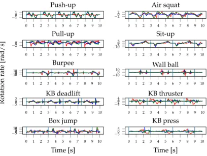
We then move on from the creative realm of music generation to the some- what more practical domain of human activity recognition (HAR) for sports using body-worn inertial sensors. We are especially interested in using off- the-shelf devices such as smartwatches, since they are becoming more and more ubiquitous. Furthermore, there is a definite interest in applications for tracking one’s workouts; society as a whole seems to be becoming more health conscious, which is also signified by an increase in commercial fitness devices and application in recent years. While most devices have a range of sensors, the most important ones for activity tracking applications are those within the Inertial Measurement Unit (IMU), namely accelerometer, gyro- scope and sometimes the magnetometer (compass). Just like music, the data from the IMU is of sequential nature. However, whereas for music we were dealing with the symbolic MIDI representation, sensor data is more akin to raw audio waves. Also, while in the first part of this dissertation our focus lies on generative tasks, in this part we are trying to discriminate between different types of movements.
In Chapter 8 we use off-the shelf smartwatches to collect data from roughly 40 CrossFit athletes of all levels while they were performing ten different ex- ercises. In order to improve data quality and minimize possible errors dur- ing the data annotation phase, as well as get accurate labels for repetition counting, we propose a constrained workout setting. In this setting, the par- ticipants are not completely free to perform the repetitions of a particular exercise, but instead they wait for a vibration signal from the smartwatch.
This way we know exactly when a repetition has started, and labelling can partly be automated. We verify that this constrained setting still generalizes well to realistic unconstrained workouts, and we believe that the use of such
constrained data collection schemes has a lot of potential for crowd-sourcing HAR datasets. Other contributions include a novel way of counting repeti- tions using a neural network that recognizes the beginning of repetitions, as well as an ablation study including smartwatches worn on both wrist and ankle. While HAR for strength training related exercises is still in its infancy, there have already been commercial solutions for swimming tracking for a while. For example, the Apple Watch supports swimming recognition, and special purpose sensors such as the Moov [5] exist as well. However, from discussions with the swimming team of our university we found that none of the existing solutions were adequate for serious swimming training. In par- ticular, the swimmers wanted an application that can help them follow a pre- defined swimming plan. This includes the requirements for highly accurate swimming style recognition, also when multiple styles are swum within the same lane, as well as turn recognition. In Chapter 9 we tackle this challenge by collecting a large dataset from roughly 50 swimmers swimming all major styles. We achieve very high recognition accuracy as well as arguably state of the art results for turn recognition (fair comparison to other work is difficult since most datasets are not publicly available). The results are promising and there is ongoing work to bring the proof of concept into production.
1.3 Understanding Neural Networks for NLP
Now, after all that workout for our muscles, our brain wants to get back in on the action. Much of how we perceive the world and communicate and interact within it is done through language, which is one of the main func- tions our brain performs every day. However, as amazing as our brain might be, it is still limited in terms of raw processing power. Luckily, we can now let computers do the heavy lifting. It is therefore no wonder that there has been a continued effort to bring computers and human language together, and in particular, to teach computers how to understand human language.
In this field, as in many others, deep learning had a transformative impact and novel applications and state of the art results have been appearing at an astonishing rate. While strong results in the latest language understand- ing benchmark are impressive and enable novel applications, the power of neural networks also comes with some downsides. In particular, as mod- els get deeper and ever more complex, we understand them less and less.
This is particularly vexing in the area of natural language processing (NLP), since it has a lot of potential for applications in, e.g., medical and legal do- mains, where interpretability and explainability are paramount. In the last part of this dissertation we investigate neural networks for NLP with the aim
of gaining a better understanding of these black boxes. True to the theme of this thesis, natural language is another type of sequential data.
In particular, in Chapter 11 we analyze the latent space of sequence-to- sequence language models based on (variational) autoencoders. We find that by adding auxiliary tasks such as translation and part-of-speech (POS) tag- ging we can change the properties of the latent space. We find that sentences of different syntactical structures get more separated in the latent space as we add more auxiliary tasks. This is encouraging, since it means that even though these neural networks have millions of parameters, they still seem to behave in a somewhat predictable and understandable manner when we add bottleneck constraints. We further find that our character-based models en- able some vector algebra operations on entire sentences, similar to the canon- ical Word2Vec examples [91].1 While our models in Chapter 11 are based on RNNs, a new neural network architecture has since taken over NLP; the transformer [141]. Transformers have even more parameters than any mod- els up to that point, and there are now models such as Microsoft’s Turing- NLG [11] with 17 billion parameters. While the increase in model size has so far led to better performance on benchmarks, the models are getting ever more opaque. One particularly popular and successful transformer variant called BERT [48] has been subject to a lot of work on interpreting and ana- lyzing transformers. In Chapter 12 we contribute to this ongoing work by challenging commonly held assumptions underlying work on drawing con- clusions about transformers based on analyzing and visualizing the learned attention distributions at different points in the model. One feature of the self-attention operation is that it updates the internal word representations by aggregating information from all other words in the input. Thus, the in- ternal word representations are mixtures of the entire input, and in deeper layers the mixing becomes stronger. Much prior work on analyzing trans- formers has assumed that a hidden token still represents the original input word as it passes throughout the model. We take an important step towards verifying this assumption, and at the same time we show that the mixing of information is indeed very strong. We therefore suggest to use more princi- pled explanation methods, such as gradient attribution, instead of inspecting attention distributions, in order to explain transformers.
1For example, the difference vector ofqueenandkingmight roughly equal that ofwomanand man.
Automatic Music Generation and Genre Transfer
7
In this part we present contributions to automatic music composition and musical style transfer. Chapter 3 introduces JamBot, a model based on hier- archical recurrent neural networks (RNN) that composes music in a human- like manner. Most interestingly, JamBot learns chord embeddings that, when plotted in two dimensions, correspond almost perfectly to the circle of fifths from music theory. While JamBot’s architecture is well suited for modeling sequential data, it is trained in a discriminative fashion and requires input seeds for generation. A more elegant, and arguably better, approach is to use a deep generative model such as a variational autoencoder (VAE). Chap- ter 4 thus presents MIDI-VAE, a recurrent VAE with parallel encoders/de- coders and shared latent space. MIDI-VAE can generate music from scratch, as well as combine songs into mixtures and medleys. MIDI-VAE also intro- duces a novel music representation based on piano rolls that simultaneously models not only the pitches of notes, but also note duration, note velocity (loudness) as well as instrumentation. In addition, MIDI-VAE is to the best of our knowledge the first approach capable of performing genre transfer on symbolic (MIDI) music. The concept of musical genre transfer can simply be understood as automatically transforming a source piece from one genre, e.g., Jazz, to another genre, e.g., Classical music. Intuitively, we want to keep the melody of the original piece mostly intact, but change the accompani- ment to match the target genre. While MIDI-VAE can be used to perform genre transfer, it is not explicitly trained with this objective. Thus, in Chap- ter 5 we adapt the CycleGAN model to the task of music genre transfer and show that it is indeed possible to achieve good genre transfer performance using a GAN-based model. For both MIDI-VAE and the CycleGAN based approach we use separately trained genre classifiers to evaluate the genre transfer performance. The use of genre classifiers is convenient as it allevi- ates the need for human evaluation or complex hand-crafted metrics. How- ever, it does not capture whether the source music piece is still recognizable at all. In other words, a model that completely ignores the source piece and just learns to generate music in the target genre can get a high score based on the genre classifier metric, but would obviously be incapable of performing actual genretransfer. Thus, Chapter 6 introduces a simple content retention metric that correlates well with human perception. Additionally, we build on the CycleGAN model introduced in Chapter 5 and investigate whether recent methods to stabilize GAN training have any positive effect on genre transfer performance.
Related Work and Background 2
In the following we will discuss related work on symbolic music generation as well as style and domain transfer. Further, we provide some background on music theory and on the symbolic music representation used in all chap- ters in this part.
2.1 Automatic Music Generation
Researchers have been trying to compose music with the help of computers for decades. One of the most famous early examples is “Experiments in Musi- cal Intelligence” [43], a semi-automatic system based on Markov models that is able to create music in the style of a certain composer. Soon after, the first attempts at music composition with artificial neural networks were made.
Most notably, Todd [135], Mozer [97] and Eck et al. [53] all used Recurrent Neural Networks (RNN). More recently, Boulanger-Lewandowski et al. [21]
combined long short term memory networks (LSTMs) and Restricted Boltz- mann Machines to simultaneously model the temporal structure of music, as well as the harmony between notes that are played at the same time, thus being capable of generating polyphonic music. There have been only few approaches that explicitly take chord progressions into account, like we do in Chapter 3. Choi et al. [37] propose a text based LSTM that learns relation-
9
ships within text documents that represent chord progressions. Chu et al. [41]
present a hierarchical recurrent neural network where at first a monophonic melody is generated, and based on the melody chords and drums are added.
It is worth noting that they incorporate the circle of fifths as a rule for generat- ing the chord progressions, whereas our model is able to extract the circle of fifths from the data. Similarly to the chord embeddings of JamBot (cf. Chap- ter 3), Huang and Wu [64] experiment with learning embeddings for notes.
The visualized embeddings show that the model learned to distinguish be- tween low and high pitches. Hadjeres et al. [59] introduce an LSTM-based system that can harmonize melodies by composing accompanying voices in the style of Bach Chorales, which is considered a difficult task even for professionals. Johnson et al. [68] use parallel LSTMs with shared weights to achieve transposition-invariance (similar to the translation-invariance of CNNs). Chuan et al. [42] investigate the use of an image-based Tonnetz rep- resentation of music, and apply a hybrid LSTM/CNN model to music gener- ation.
Generative models such as the Variational Autoencoder (VAE) [72] and Generative Adversarial Networks (GAN) [57] have become increasingly suc- cessful at generating music. The introduction of these generative models has led to numerous works in the visual domain. Progress has been slower in sequence tasks, but the pace has recently picked up, and increasingly more works are now based on generative models. Google Brain’s Magenta project [2] has introduced a range of approaches based on generative mod- els for the generation of symbolic music. Roberts et al. introduced Music- VAE [118], a hierarchical VAE model that can capture long-term structure in polyphonic music and exhibits high interpolation and reconstruction perfor- mance. They use fixed instrument assignments and treat drums separately, whereas our model, MIDI-VAE, (cf. Chapter 4) is also based on a VAE, but can learn arbitrary instrument mappings that do not need to be defined be- forehand. GANs, while very powerful, are notoriously difficult to train and have initially not been applied to sequential data. However, Mogren [93], Yang et al. [152] and Dong et al. [51] have shown the efficacy of CNN-based GANs for music composition. Yu et al. [155] successfully applied RNN-based GANs to music by incorporating reinforcement learning techniques. We use CNN-based GANs to model music and perform domain transfer (cf. Chap- ter 5).
2.2 Style and Domain Transfer
Gatys et al. [55] introduced the concept of neural style transfer and show that pre-trained CNNs can be used to merge the style and content of two im-
ages. For sequential data, autoencoder based methods [124, 159] have been proposed to change the sentiment or content of sentences. Van den Oord et al. [140] introduce a VAE model with discrete latent space that is able to perform speaker voice transfer on raw audio data. Mor et al. [94] develop a system based on a WaveNet autoencoder [54] that can translate music across instruments, genres and styles, and even create music from whistling. Ma- lik et al. [89] train a model to add note velocities (loudness) to sheet music, resulting in more realistic sounding playback. Their model is trained in a su- pervised manner, with the target being a human-like performance of a music piece in MIDI format, and the input being the same piece but with all note velocities set to the same value. While their model can indeed play music in a more human-like manner, it can only change note velocities, and does not learn the characteristics of different musical styles/genres. MIDI-VAE (cf. Chapter 4) is trained on unaligned songs from different musical genres.
MIDI-VAE can not only change the dynamics of a music piece from one style to another, but also automatically adapt the instrumentation and even the note pitches themselves.
Approaches such as CycleGAN [160] use a pair of generators to transform data from a domain A to another domain B. The nature of the two domains implicitly specifies the kinds of features that will be extracted. For example, if domain A contains photographs and domain B contains paintings, then CycleGAN should learn to transfer any painting into a photograph and vice versa. We use the same structure as CycleGAN (cf. Chapter 5) and apply it to music in the MIDI format. The general idea of CycleGAN has been fur- ther developed and improved. A few notable examples include CycleGAN- VC [69], StarGAN [39], CoGAN [81] and DualGAN [154]. In the future more complex architectures should be investigated but in this thesis we focus on showing the feasibility of a CycleGAN approach to domain transfer for sym- bolic music.
2.3 Music Theory Primer
Here we introduce some important principles from music theory that we use in subsequent chapters. This is a very simplistic introduction, and we refer the reader to standard works such as [90] for an in-depth overview.
In musical notation, abarormeasureis a segment of time corresponding to a specific number of beats. Each beat corresponds to a note value. The boundaries between bars (hence the name) are indicated by vertical lines. In most, but not all music a bar is 4 beats long.
Almost all music uses a 12 tone equal temperament system of tuning, in which the frequency interval between every pair of adjacent notes has the
same ratio. Notes are: C,C]/D[,D, D]/E[,E,F,F]/G[,G, G]/A[, A,H, and then againCone octave higher. One cycle (e.g.,Cto nextC) is called an octave. Notes from different octaves are denoted with a number, for example D6 is theDfrom the sixth octave.
Ascaleis a subset of (in most cases) 7 notes. Scales are defined by the pitch intervals between the notes of the scale. The most common scale is the major scalewith the following pitch intervals: 2, 2, 1, 2, 2, 2, 1. The first note of the scale is called theroot note. The pair of root note and scale is called a key. The major scale with the root noteCcontains the following notes:
C−→2 D−→2 E−→1 F−→2 G−→2 A−→2 H−→1 C.
Thenatural minorscale has different pitch intervals than the major scale, but a natural minor scale with root note Acontains exactly the same notes as a major scale with root noteC. This is called arelative minor.
Achordis a set of 3 or more notes played together. Chords are defined, like keys, by the pitch intervals and a starting note. The two most common types of chords aremajor chordsandminor chords. We denote the major chords with the capital starting note, e.g.,Ffor anFmajor chord. For minor chords we add anm, e.g.,Dmfor aDminor chord.
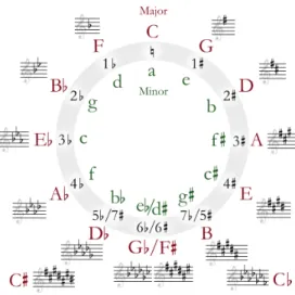
Thecircle of fifths, which is shown in Figure 2.1, is the relationship among the 12 notes and their associated major and minor keys. It is a geometrical representation of the 12 notes that helps musicians switch between different keys and develop chord progressions. Choosing adjacent chords to form a chord progression often produces more harmonic sounding music.
2.4 Symbolic Music and MIDI
All of the work presented in this thesis uses a symbolic representation of music based on so-called MIDI files. MIDI (Musical Instrument Digital In- terface) [4] was originally created as a standard communication interface be- tween electrical instruments, computers and other devices. Thus, MIDI files do not contain actual sound like MP3 files, but instead so-called MIDI mes- sages. For our purposes, the most relevant ones are theNote OnandNote Off messages. TheNote Onmessage indicates that a note is beginning to be played, and it also specifies the velocity (loudness) of that note. TheNote Off message denotes the end of a note. Each note also has a specified pitch, which in MIDI can range between 0 and 127, corresponding to a note range ofC−1toG9. A standard piano can play MIDI notes 21 to 108, or equivalently A0toC8. Velocity values also range between 0 and 127. MIDI messages may be sent on different channels which have different instruments assigned to
Figure 2.1: Circle of fifths, a visualization of the relationship between the 12 notes as it is used by musicians.
them. For example channel 0 may represent a piano while channel 1 corre- sponds to a guitar. Because MIDI files only contain a score (sheet music) of the song and no actual sound, a song usually takes much less storage space than other audio files such as WAV or MP3. Furthermore, the MIDI format already provides a basic representation of music, whereas a raw audio file is more difficult to interpret, for humans as well as machine learning algo- rithms. Since MIDI files do not contain any sounds themselves, a MIDI syn- thesizer is required to actually play them, which makes it easy to change the instrument with which the music is played. Such synthesizers can either be hardware devices or pieces of software. The final sound will depend on the implementation of the instrument sounds within the used synthesizer.
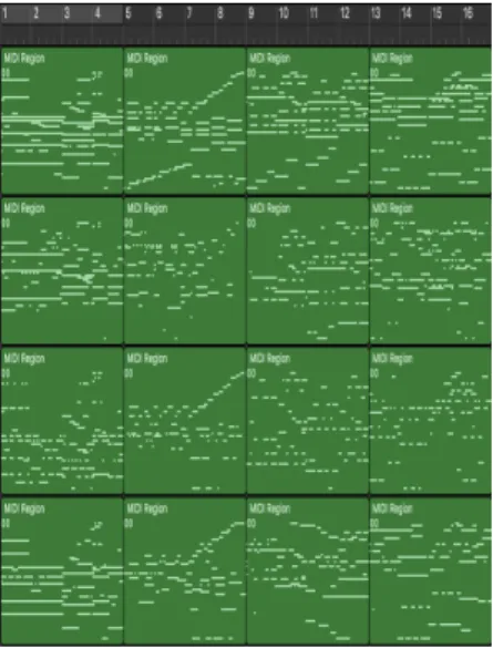
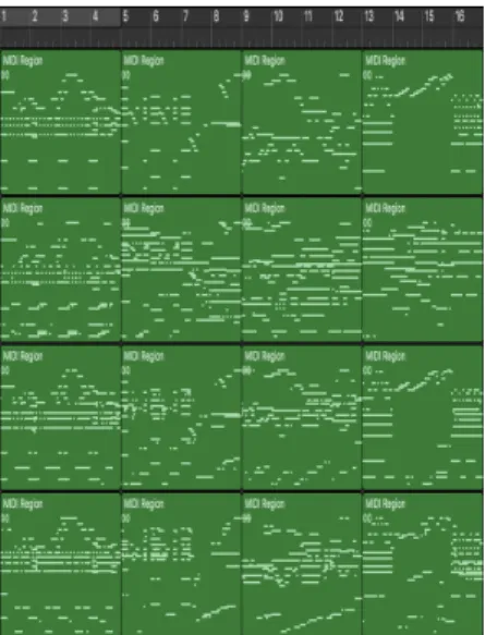
In order to actually train neural networks using data from MIDI files we need to convert them into matrix form. The most basic form is the so-called piano roll which gets its name from the actual physical piano roll used in automatic pianos, but has since also been used to refer to digital represen- tations of MIDI files [6]. In the context of machine learning for music, we use the term piano roll for a matrix where one dimension represents time, and the other represents pitch. In particular, there is ak-hot vector for each
time step that encodes which notes are being played. The basic pianoroll rep- resentation only supports single instruments and cannot encode notes that are held across time steps. In the following chapters we use slightly differ- ent versions of the piano roll; in Chapters 3, 5 and 6 we use the basic piano roll as just described. In Chapter 4 we propose a novel symbolic music rep- resentation based on piano rolls that can encode multiple instruments and note durations. We will provide more detailed descriptions of the specific implementations in the respective chapters.
JamBot: Automatic Composition of 3
Music Using Hierarchical Recurrent Neural Networks
In this chapter we introduceJamBot1, a music theory aware system for the generation of polyphonic music. JamBot consists of two hierarchically ar- ranged LSTMs. First, thechord LSTMgenerates a chord progression which serves as the long-term structure for the music piece. The chord sequence is then fed into thepolyphonic LSTMthat generates the individual notes. The polyphonic LSTM is free to predict any note, not just chord notes. The chords are only provided as information to the LSTM, not as a rule. JamBot man- ages to produce harmonic sounding music with a long time structure. When trained on MIDI music in major/natural minor scales with all twelve keys, our model learns a chord embedding that corresponds strikingly well to the circle of fifths. Thus, our LSTM is capable of extracting an important concept of music theory from the data.
1Music samples and our code can be found at www.youtube.com/channel/
UCQbE9vfbYycK4DZpHoZKcSwandhttps://github.com/brunnergino/JamBotrespectively
15
0 10 20 30 40 50 60 70 80 90 100 0
0.5 1
·106
Pitch
Occurrences
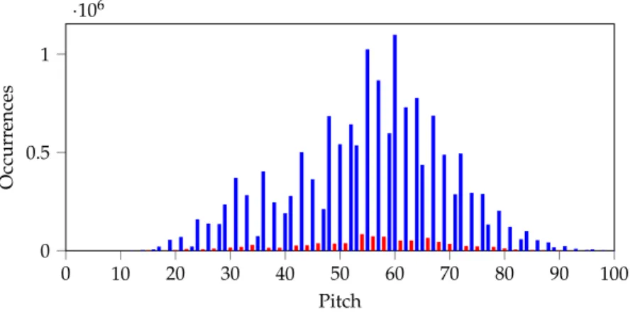
Figure 3.1: Histogram over the notes of the shifted dataset. The notes that belong to theCmajor/Aharmonic minor scale are blue, the others red.
3.1 Dataset
To train JamBot we use a subset of the Lakh MIDI Dataset [112]. The dataset contains approximately one hundred thousand songs in the MIDI data for- mat. To analyze the scales and keys of the songs we consider 5 scale types:
Major, natural minor, harmonic minor, melodic minor and the blues scale.
Because the major scale and its relative natural minor scale contain the same notes and only the root note is different, we treat them as the same major/rel- ative minor scale in the preprocessing. Every scale can start at 12 different root notes, so we have 4·12 = 48 different possible keys. To find the root notes and scale types of the songs we compute a histogram of the twelve notes over the whole song. To determine the keys, the 7 most occurring notes of the histograms were then matched to the 48 configurations. Analyzing the 114,988 songs of the dataset shows that 86,711 of the songs are in the major/relative minor scale, 1,600 are in harmonic minor, 765 are in the blues scale and 654 are in melodic minor. The remaining 25,258 are in another scale, there is a key change in the song or the scale could not be detected correctly with our method. If the key changes during a song, the histogram method possibly detects neither key. Also, if a non scale note is played often in a song, the key will also not be detected correctly. To simplify the music gener- ation task, we use only the songs in the major/minor scales as training data, since they make up most of the data. Additionally those songs are shifted to the same root noteCwhich corresponds to a constant shift of all the notes
in a song. We call this dataset theshifted datasetfrom now on. This way the models only have to learn to create music in one key instead of twelve keys.
This step is taken only to avoid overfitting due to a lack of data per key. After generation, we can transpose the song into any other key by simply adding a constant shift to all the notes. If a song sounds good in one key, it will also sound good in other keys. Figure 3.1 shows a histogram of all the notes in the shifted dataset. We notice that most of the notes belong to the scale, but not all of them. Therefore, simply ignoring the notes that do not belong to the scale and solely predicting in-scale notes would make the generated music
“too simplistic”. In real music, out of scale notes are played, e.g., to create tension. MIDI has a capacity of 128 different pitches fromC-1 toG9. Fig- ure 3.1 shows that the very high and the very low notes are not played often.
Because of the lack of data in these ranges and since very low and very high notes usually do not sound pleasant, we only use the notes fromC2 toC6 as training data.
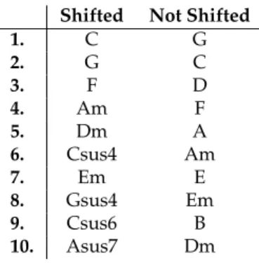
In order to train the chord LSTM (see Section 3.2.2), we need to extract the chords from the songs. Because it is not feasible to determine the chords manually, we automate the process. To that end, we compute a histogram of the 12 notes over a bar. The three most played notes of the bar make up the chord. The length of one bar was chosen because usually in popular music the chords roughly change every bar. Of course this is only an approximation to a chord as it is defined in music theory. We only consider chords with up to three notes, even though there are chords with four or more notes. Our method might also detect note patterns that are not chords in a music theo- retical sense, but appear often in real world music. For example, if a note that is not a note of the current chord is played more often than the chord notes, the detected chord might vary from the true chord. In Table 3.2 the 10 most common chords of the extracted chord datasets can be seen. In both datasets the most common chords are what one might expect from large datasets of music, and the extracted chords agree with [32], [34] and [8]. Therefore we conclude that our chord extraction method is plausible.
3.2 Model Architecture
When you listen to a song, temporal dependencies in the song are impor- tant. Likewise, as you read this paragraph, you understand each word based on your understanding of the context and previous words. Classical neu- ral networks, so-called Multi Layer Perceptrons(MLP), cannot do this well.
Recurrent neural networks (RNN) were proposed to address this issue, how- ever, normal RNNs usually only capture short-term dependencies. In order to add long-term dependencies into generated music, which is believed to be
Table 3.2:The 10 most frequent chords in the shifted and the original dataset.
Shifted Not Shifted
1. C G
2. G C
3. F D
4. Am F
5. Dm A
6. Csus4 Am
7. Em E
8. Gsus4 Em
9. Csus6 B
10. Asus7 Dm
a key feature of pleasing music, we use LSTM (Long Short-Term Memory) networks [63] which is an architecture designed to improve upon the RNN with the introduction of memory cells with a gating architecture. These gates decide whether LSTM cells should forget or persist the previous state in each loop and thus make LSTMs capable of learning dependencies across longer sequences.
We denote byx0, . . . ,xt, . . . the input sequences andy0, . . . ,yt, . . . the out- put sequences. For each memory cell, the network computes the output of four gates: an update gate, input gate, forget gate and output gate. The out- puts of these gates are:
i=σ(Uixt+Viht−1) f =σ(Ufxt+Vfht−1) o=σ(Uoxt+Voht−1) g=tanh(Ugxt+Vght−1)
where Ui,Uf,Uo,Ug,Vi,Vf,Vo,Vg are all weight matrices. The bias terms have been omitted for clarity. The memory cell state is then updated as a function of the input and the previous state:
ct =fct−1+ig.
The hidden state is computed as a function of the cell state and the output gate, and finally the output is computed as the output activation functionδ
pre pro- cessing
chords piano rolls
chord LSTM
polyphonic LSTM
generated chord pro- gression
tempo instrumentation
input MIDI training data
extract
extract
train
train
train generate
input generate MIDI
Figure 3.3: The architecture of JamBot. Chords and piano roll representa- tions are extracted from the MIDI files in the training data (in black). The extracted chords and piano rolls are then used to train the chord and poly- phonic LSTMs (in red). During music generation (in blue), the chord LSTM generates a chord progression that is used as input to the polyphonic LSTM which generates new music in MIDI format. When listening to the music, one can freely vary tempo and instrumentation.
of the output matrixWoutmultiplied with the hidden state:
ht =otanh(ct) yt=δ(Woutht)
For more details about LSTMs, we refer the interested reader to [56]. In Figure 3.3 JamBot’s architecture is shown. We will explain it in detail in the following.
3.2.1 Input Data Representation
To represent the music data that is fed into thepolyphonic LSTMwe use api- ano rollrepresentation. Every bar is divided into eight time steps. The notes that are played at each time step are represented as a vector. The length of these vectors is the number of notes. If a note is played at that time step, the corresponding vector entry is a 1 and if the note is not played the correspond- ing entry is a 0. The piano rolls of the songs are created with the pretty_midi library [113].
0 50 100 150 200 250 300 0
0.5 1
·106
Chords
Occurrences
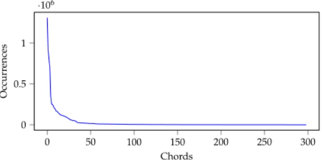
Figure 3.4: This figure shows the number of occurrences of all 300 unique chords in the shifted dataset.
To represent thechords of a song we use a technique from natural lan- guage processing. In machine learning applications that deal with language, words are often replaced with integer ids and the word/id pairs are stored in a dictionary. The vocabulary size is usually limited. Only theNmost occur- ring words of a corpus receive a unique id, because the remaining words do not occur often enough for the algorithms to learn anything meaningful from them. The rarely occurring words receive the id of anunknown tag. For the chord LSTMwe use the same technique. The chords are replaced with ids and the chord/id pairs stored in a dictionary. Thus, the chord LSTM only sees the chord ids, but has no knowledge of the notes that make up the chords. Fig- ure 3.4 shows the number of occurrences of all unique chords in the shifted dataset. On the left is the most frequent chord and on the right the least fre- quent one. Even though there are 12·11·10+12·11+12=1, 465 different possible note combinations for 3, 2 or 1 notes, there are only 300 different combinations present in the shifted dataset. This makes sense since most random note combinations do not sound pleasing, and thus do not occur in real music. It can be seen that few chords are played very often and then the number of occurrences of the chords drops very fast. Based on this data the vocabulary size was chosen to be 50. The remaining chords received the id of the unknown tag. Before we can feed the chord ids into the chord LSTM we have to encode them as vectors. To do so we use one-hot encoding. The input vectors are the same size as the size of the chord vocabulary. All the vector entries are 0, except for the entry at the index of the chord id which equals 1.
3.2.2 Chord LSTM Model
For the first layer of the chord LSTM we used another technique from nat- ural language processing; input embeddings. This technique has been pio- neered by Bengio et al. [20] and has since been continuously developed and improved [91]. In natural language processing, a word embedding maps words from the vocabulary to vectors of real numbers. Those embeddings are often not fixed, but learned from the training data. The idea is that the vector space can capture relationships between words, e.g., words that are semantically similar are also close together in the vector space. For example, the days of the week, or words like king and queen, might be close together in the embedding space. For the chords we used this exact same technique. The one-hot vectorsxchord (cf. Section 3.2.1) are multiplied with an embedding matrixWembed, resulting in a 10-dimensional embedded chord vector:
xembed=Wembed·xchord
The hope is that the chord LSTM learns a meaningful representation of the chords from the training data. In our LSTM the embedding matrixWembed consists of learnable parameters. Those parameters are trained at the same time as the rest of the chord LSTM. After the embedding layer, the embedded chords are fed into an LSTM with 256 hidden cells. We use softmax as the activation function of the output layer. Thus, the output of the LSTM is a vector that contains the probabilities for all the chords to be played next.
To train the chord LSTM we use cross-entropy as loss function and the Adam optimizer [71]. The best initial learning rate we found was 10−5. The training data consists of the extracted chords of 80,000 songs from the shifted dataset. We trained the model with this data for 4 epochs. We also trained a second chord LSTM with the extracted chords of 100’000 songs from the original unshifted dataset to visualize the embeddings that it learned.
To predict a new chord progression, we first feed a seed of variable length into the LSTM. The next chord is then predicted by sampling from the out- put probability vector with temperature. The predicted chord is then fed back into the LSTM and the next chord is sampled, and so on. The temperature pa- rameter controls how diverse the generated chord progression is by scaling the logits before the softmax function. A higher temperature will generally result in more “interesting” music, but will also lead to more wrong/disso- nant notes.
3.2.3 Polyphonic LSTM Model
The input vector of the polyphonic LSTM can be seen in Figure 3.5. It consists of the vectors from the piano rolls of the songs (cf. Section 3.2.1) with addi-
xtpoly=
0
... 3.579
... 0.256
... 1 ...
)
Piano roll )
Chord )
Next Chord )
Counter
Figure 3.5:The input vector of the polyphonic LSTM at timet. It consists of the piano roll vector, the embedded current chord, the embedded next chord and the counter.
ytpoly=
P(n0=1|x0poly,· · ·,xt−1poly) ...
P(nN =1|x0poly,· · ·,xt−1poly)
Figure 3.6:The output vector of the polyphonic LSTM at timet.
tional features appended. The first additional feature is the chord embedding of the next time step. The embedding is the same as in the completely trained chord LSTM described in Section 3.2.2. With the chord of the notes to be pre- dicted given, the LSTM can learn which notes are usually played to which chords. This way the predicted notes follow the chord progression and the generated songs receive more long term structure. In music the melodies of- ten “lead” to the next chord. For this reason we also append the embedding of the chord which follows the next chord. This should cause the generated songs to be more structured. The last feature that is appended is a simple binary counter that counts from 0 to 7 in every bar. This helps the LSTM to know at which time step in the bar it is and how many steps remain to the next chord change. This should make the chord-transitions smoother.
The input vectors are fed into an LSTM with 512 cells. The activation function of the output is a sigmoid. The output of the LSTM at timetytpoly can be seen in Figure 3.6. It is a vector with the same number of entries as there are notes. Every output vector entry is the probability of the cor- responding note to be played at the next time step, conditioned on all the
inputs of the time steps before. The polyphonic LSTM is trained to mini- mize the cross entropy loss between the output vectorsytpolyand the ground truth. We use the Adam optimizer with an initial learning rate of 10−6. Since for every time step in the chord LSTM there are 8 time steps in the poly- phonic LSTM, the training data for the polyphonic LSTM only consists of 10,000 songs from the shifted dataset in order to reduce training time. We trained the LSTM for 4 epochs.
To predict a new song we first feed a seed consisting of the piano roll and the corresponding chords into the LSTM. The notes which are played at the next time step are then sampled using the output probability vectorytpoly. The notes are sampled independently, so if one note is chosen to be played, the probabilities of the other notes do not change. We also implement a soft upper limit for the number of notes to be played at one time step. The train- ing data mainly consists of songs where different instruments are playing at the same time with different volumes. The predicted song however is played back with only one instrument and every note is played at the same volume.
So while the songs from the training data might get away with many notes playing at the same time, with our playback method it quickly sounds too cluttered. For this reason we implemented a soft upper limit for the number of notes to be played at one time step. Before prediction we take the sum of all probabilities of the output vector and if it is greater than the upper limitl, we divide all the probabilities by the sum and then multiply them byl:
s=sum{ytpoly}=
∑
N i=1P(ni=1|x0poly,· · ·,xt−1poly) ytpoly
new=ytpoly·(l/s)
This prevents us from sampling too many notes to be played simultaneously.
We foundl=5 to work well in our experiments.
In the piano roll representation there is no distinction between a note that is held forttime steps and a note played repeatedly forttime steps. So it is up to us how to interpret the piano roll when replaying the predicted song.
We found that it generally sounds better if the notes are played continuously.
To achieve this, we merge consecutive notes of the same pitch before sav- ing the final MIDI file. However, at the beginning of each bar all notes are repeated again. This adds more structure to the music and emphasizes the chord changes. The instrumentation and the tempo at which the predicted songs are played back with can be chosen arbitrarily. Thus, the produced music can be made more diverse by choosing different instruments, e.g., pi- ano, guitar, organ, etc. and varying the tempo that is set in the produced MIDI file.
3.3 Results
In this section we investigate the chord embeddings which the chord LSTM has learned, and also briefly discuss the qualities of the generated music.
3.3.1 Learned Chord Embeddings
The most interesting result from the chord LSTM are the embeddings it learned from the training data. To visualize those embeddings we used PCA (Princi- pal Component Analysis) to reduce the ten dimensional embeddings of the chords to two dimensions. In Figure 3.7 we can see a plot of the visualized embeddings of a chord LSTM that was trained with the original unshifted dataset. The plot contains all the major chords from the circle of fifths, which we can see in Figure 2.1. Interestingly the visualized embeddings form ex- actly the same circle as the circle of fifths. So the chord LSTM learned a repre- sentation similar to the diagram that musicians use to visualize the relation- ships between the chords. Thus, our model is capable of extracting concepts of music theory from data.
In contrast to previous methods such as [41] where domain knowledge is used explicitly to help the system do post-processing (i.e., to produce the chords with the circle of fifths), our method automatically mines this knowl- edge from the dataset and then, arguably, exploits this mined theory to gener- ate music. Actually, these two learning methods are also similar to the ways in which human-being learns. A human musician either learns the theory from her teacher, or learns by listening to a number of songs and summa- rizing a high level description and frequent patterns of good music. At a first glance, the first way appears more efficient, but in most cases encoding knowledge into a machine-readable way manually is difficult and expensive, if not impossible. Besides, the second learning way may help us extend the current theory by finding some new patterns from data.
In Figure 3.8 we used the same technique to visualize the chord embed- dings trained on the shifted dataset. The embeddings of the 15 most occur- ring chords are plotted. Instead of the chord names the three notes that make up each chord are shown. We can see that chords which contain two common notes are close together. It makes sense that chords that share notes are also close together in the vector space. The chord progressions predicted by the chord LSTM contain structures that are often present in western pop music.
It often repeats four chords, especially if the temperature is set low. If the temperature is set higher, the chord progressions become more diverse and there are fewer repeating structures. If the sampling temperature is low, the predicted chords are mostly also the ones that occur the most in the training
−3
−2
−1 0 1 2 3
−3
−2
−1 0 1 2 3
D[
A[
E[
B F
C
G
D
EA
H G[,/F
Figure 3.7:Chord embeddings of the chord LSTM trained with the original, unshifted dataset. The learned embedding strongly resembles the Circle of Fifths. The 10 dimensional embeddings were reduced to 2 dimensions with PCA.
data, i.e., from the Top 10 in Table 3.2. If the sampling temperature is high the less occurring chords are predicted more often.
3.3.2 Music Generation
The songs generated by the polyphonic LSTM sound quite pleasant. There clearly is a long term structure in the songs and one can hear distinct chord changes. The LSTMs succeeded in learning the relationship between the chords and which notes can be played to them. Therefore it is able to generate polyphonic music to the long term structure given by the predicted chords.
The music mostly sounds harmonic. Sometimes there are short sections that sound dissonant. That may be because even if the probabilities for playing dissonant notes are small, it can still happen that one is sampled from time to time. Sometimes it adds suspense to the music, but sometimes it just sounds wrong. With a lower sampling temperature for the chord LSTM, the songs sound more harmonic but also more boring. Accordingly, if the sampling temperature is high, the music sounds less harmonic, but also more diverse.
This might be because the chord LSTM predicts more less occurring chords