Compression of Matrices with Multi-Terminal Decision Diagrams

Goethe Universität Frankfurt am Main Institut für Informatik

Wintersemester 2018/2019

Bachelor‘s thesis

Compression of Matrices with Multi-Terminal Decision Diagrams

Emre Cümbüş

Supervisor: Prof. Dr. Manfred Schmidt-Schauß

Due Date: 22.11.2018

Erklärung

gemäß § 25, Abs. 11 der Ordnung für den Bachelorstudiengang Informatik vom 06. Dezember 2010:

Hiermit erkläre ich, dass ich die vorliegende Arbeit selbstständig und ohne Benutzung anderer als der angegebenen Quellen und Hilfsmittel verfasst habe. Ebenso bestätige ich, dass diese Arbeit nicht,

auch nicht auszugsweise, für eine andere Prüfung oder Studienleistung verwendet wurde.

Frankfurt am Main, 22.11. 2018 Emre Cümbüş

………

Ort und Datum

………..

Unterschrift

Acknowledgements

I would like to thank everyone who supported me throughout this project:

My supervisor, Prof. Dr. Schmidt-Schauß for guiding and supporting me.

Dr. Dermot O`Brien for examining this thesis as well as making suggestions for improvement.

Contents

1 Introduction ...1

2 Preliminaries ...1

2.1 Grammar for Compression of Matrices ...2

2.1.1 +MTDD - Grammar ...2

2.2 Linear Algebra ...4

2.2.1 Basics ...4

2.2.2 Linear Equations ...7

2.2.3 Gaussian Elimination ...8

2.3 Combinations ...9

2.4 Haskell ... 10

3 Enhanced +MTDD – Grammar ... 10

4 Implementations using Haskell ... 12

4.1 Implementing the +MTDD – Grammar ... 13

4.1.1 Data Structure ... 13

4.1.2 Overview Functions ... 14

4.2 Implementing Enhanced +MTDD – Grammar... 14

4.2.1 Data Structure ... 14

4.2.2 Overview of Functions ... 15

4.2.3 Creating an Enhanced +MTDD Grammar using toMatrixGrammarEnhanced ... 17

4.2.4 Finding Solutions and Sub-solutions using Gauss Elimination ... 19

4.2.5 Checking Combinations ... 23

4.2.6 Get Element ... 26

4.2.7 Creating an Enhanced +MTDD Grammar from a List of Matrices ... 29

5 Analysis ... 32

5.1 Time Complexity Analyze... 32

5.1.1 toMatrixGrammarEnhanced ... 32

5.1.2 getElementEnhanced ... 33

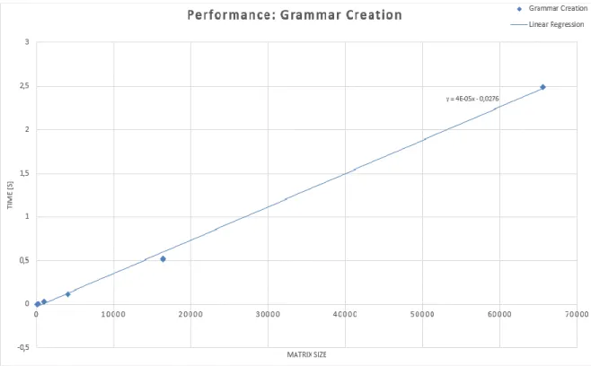
5.2 Performance ... 33

6 Conclusion and Future Work ... 37

Bibliography... 38

Function Descriptions ... 39

1

1 Introduction

Data compression is playing an important role in many areas of computer science. According to an infographic by Nasuni (Nasuni Corporation, 2016), the average cost to store one terabyte of file data per year is 3,351 dollars. Another study, by Ben Walker, Marketing Executive at Voucher Cloud (VCloudNews, 2015), shows that everyday 2.5 million terabytes of data are created. With these numbers the yearly cost of data storage in the world amounts to 2.5 million TB * 365 * 3.351 = over 3 billion dollars. Thus, it is possible to reduce data storage costs by compressing the data first.

However, the compression comes with a computational cost and/or with some possible information loss. We can categorize data compression into two types: lossy, where the data experiences some information loss (e.g. MP3, JPEG and MPEG data formats) and lossless where there is no information loss after the compression is done. Due to its computational costs, it is important for a compression algorithm to compress and decompress a given data-flow efficiently. To be able to discuss any compression algorithm, one should define the type of the data-flow and the category the compression algorithm belongs to.

In subsection 2.1.1, we define Multi-Terminal Decision Diagram with Addition (+MTDD), which is used for lossless compressing square matrices of form 2^𝑘× 2^𝑘, 𝑘 ∈ 𝑘. Moreover, we extend the data structure of +MTDD and present Enhanced Multi-Terminal Decision Diagram with Addition (Enhanced +MTDD) in section 3, which allows us to represent non-terminal symbols with other non-terminal symbols using linear equations and combinations. How we create linear equations and combinations using non-terminals is discussed in subsection 4.2.4 and 4.2.5 respectively. Furthermore, in

subsection 4, we implement the data structure and some useful functions for +MTDD as well as for Enhanced +MTDD using the functional programming language Haskell (In subsection 2.4, we aim to give a brief understanding on how Haskell works and which data types we use). Due to the time constraint of this thesis, we can only explain some essential functions in detail in section 4. However, a list of functions with their brief descriptions is found at the end of this document. In subsection 5.1.1 and subsection 5.1.2, we discuss the time complexities of creating an enhanced +MTDD

grammar and calculating an entry of the matrix that is represented by an enhanced +MTDD grammar respectively. Moreover, we benchmark the run-time of grammar creation and entry calculation using a library called Criterion. Criterion uses Kernel Density Estimation, which allows us to examine the distribution of run-times.

In this thesis, we put the emphasis on the implementation of the data structure as well as on the implementation of functions for Enhanced +MTDD Grammar. Not to mention that derivation of Enhanced +MTDD Grammar from +MTDD Grammar is also an integral part of the thesis.

2 Preliminaries

In this section, we introduce the preliminaries that we use in the rest of the thesis. The first

subsection aims to give a brief understanding of what a matrix grammar is. We then further discuss a matrix compression method called +MTDD (which is derived from MTDD) in the subsections 2.1.1.

Lastly, in the sections 2.2, 2.3 and 2.4 our goal is to give an overview of linear algebra, give an understanding on what we refer to with “combinations” and discuss some of the qualities of the functional programming language Haskell, respectively.

2

2.1 Grammar for Compression of Matrices

Informally, a grammar is a set of production rules, which can be recursively applied on a finite

sequence to generate new finite sequences. The finite sequence consists of nonterminal and terminal symbols. One can think of nonterminal symbols as the nodes of a tree, where with the given set of production rules, it is possible to generate another subtree or a leaf and terminal symbols as the leafs. We say, a grammar is context-free, if every generated finite sequence can be any combinations of terminal and nonterminal symbols. The formal definition of a context-free grammar (cf. Schnitger, 2018, pp. 312-317), (cf. Chiang, 2017, p. 41):

Definition 1. (Context-free grammar) A context-free grammar is a quadruple 𝐺 = (𝑁, 𝛴, 𝑃, 𝑆), where

 𝑁 is a set of nonterminal symbols

 𝛴 is a set of terminal symbols

 𝑃 is a set of production rules of the form 𝐴 → 𝛽, where 𝐴 ∈ 𝑁 and 𝛽 ∈ (𝑁 ∪ 𝛴)^∗

 𝑆 ∈ 𝑁 is a distinguished start symbol

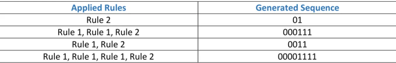
Example 1. ({0^𝑛1^𝑛, 𝑛 ≥ 1} -Generator)

Let grammar 𝐺 = ({𝑆}, {0,1}, 𝑃, 𝑆} with the production rules 1. 𝑆 → 0𝑆1

2. 𝑆 → 01

With this grammar, we can generate every 0^𝑛1^𝑛 (𝑛 ≥ 1) finite sequence.

Here are some sequences generated by this context-free grammar:

Applied Rules Generated Sequence

Rule 2 01

Rule 1, Rule 1, Rule 2 000111

Rule 1, Rule 2 0011

Rule 1, Rule 1, Rule 1, Rule 2 00001111

Table 1: Generated sequences with the grammar from Example 1.

2.1.1 +MTDD - Grammar

The ideas in this section are mainly taken from Processing Succinct Matrices and Vectors (Lohrey &

Schmidt-Schauß, 2015, pp. 323-338).

A MTDD (Multi Terminal Decision Diagram) - Grammar of height ℎ is a non-cyclical, context-free grammar used for compressing matrices of size (2^𝑛× 2^𝑛). A height 𝑖 (0 ≤ 𝑖 ≤ ℎ) describes how many replacements it takes from a nonterminal symbol, which has the height 𝑖, to reach a terminal symbol (leaf). However, the standard implementation of MTDD does not allow the addition of nonterminal symbols of height 𝑖 with (1 ≤ 𝑖 ≤ ℎ) to be represented in the grammar. In other words, only the scalars (terminal symbols) are allowed to be added. For that reason, we use an enhanced

3

version of MTDD called +MTDD (Multi Terminal Decision Diagram with Addition) - Grammar, which we formally define as follows:

Definition 2. (+MTDD Grammar) A +MTDD (Multi Terminal Decision Diagram) - Grammar 𝐺 of height ℎ is a non-cyclical, context-free grammar, where every nonterminal symbol of 𝐺 is unambiguous, meaning there is exactly one production rule for each nonterminal symbol. Let 𝑁 be the set of nonterminal symbols. We partition the set of nonterminal symbols 𝑁 into ℎ non-empty

subsets {𝑁₀, … , 𝑁_ℎ}, with 𝑁_ℎ being a singleton that contains the start symbol. Let 𝑎 be a terminal symbol of 𝐺. We can assign a height 𝑖 (0 ≤ 𝑖 ≤ ℎ) to every production rule in the grammar, so each production rule has one of the following forms:

1. 𝐴 → (𝐴_1,1 𝐴_1,2

𝐴_2,1 𝐴_2,2) , with 𝐴 ∈ 𝑁_𝑖 and 𝐴_1,1, 𝐴_1,2, 𝐴_2,1, 𝐴_2,2∈ 𝑁_𝑖−1 2. 𝐴 → 𝐴1+ 𝐴2, with 𝐴, 𝐴1, 𝐴2∈ 𝑁𝑖

3. 𝐴 → 𝑎, with 𝐴 ∈ 𝑁₀

As we can see above, due to the production rule 1, every non-terminal symbol of height 𝑖 (𝑖 ≠ 0) has four child nodes, where each child node corresponds to a non-terminal symbol of height 𝑖 − 1. To put it another way, in order for a non-terminal symbol of height 𝑖 to reach the zero level, it needs to use the rule 1 𝑖 times, which results in a 2^𝑖× 2^𝑖 matrix consisting of 4^𝑖 terminal values. For 𝑖 = ℎ, we calculate 4^ℎ terminals, which corresponds to a matrix of size 2^ℎ × 2^ℎ. Hence, the height ℎ

corresponds to the exponent 𝑛 of the represented matrix. The production rule 2 is used to represent the addition of two non-term symbols of same height. However, we can perform an addition of two non-terminal symbols only after every terminal symbol of these two non-terminals are calculated.

The production rule 3 represents the non-terminals of height zero that points to terminal symbols.

Example 2. (+MTDD Grammar)

Let 𝐺 be a +MTDD Grammar of height 2, where the start symbol 𝑆 = 𝐵₁, set of non-terminal symbols 𝑁 = {𝑁₀, 𝑁₁, 𝑁₂}, 𝑁₀= {𝑇₁, 𝑇₂, 𝑇₃, 𝑇₄}, 𝑁₁= {𝐴₁, 𝐴₂, 𝐴₃, 𝐴₄} and 𝑁₂= 𝐵₁, with the following productions:

𝐵₁→ (𝐴₁ 𝐴₂ 𝐴₃ 𝐴₄) 𝐴1 → (𝑇₁ 𝑇₂

𝑇3 𝑇4) 𝐴2→ (𝑇₂ 𝑇₂

𝑇1 𝑇4) 𝐴₃→ (𝑇₁ 𝑇₁

𝑇₁ 𝑇₁) 𝐴₄→ 𝐴₁+ 𝐴₂ 𝑇1→ 1 𝑇₂→ 2 𝑇₃→ 3 𝑇₄→ 4

We extract the represented matrix by starting with the start value:

4 𝐵₁→ (𝐴₁ 𝐴₂

𝐴₃ 𝐴₄)𝑎𝑝𝑝𝑙𝑦𝑖𝑛𝑔 𝑟𝑢𝑙𝑒 2

→ (𝐴₁ 𝐴₂

𝐴₃ 𝐴₁+ 𝐴₂)𝑎𝑝𝑝𝑙𝑦𝑖𝑛𝑔 𝑟𝑢𝑙𝑒 1

→ (

𝑇₁ 𝑇₂ 𝑇₂ 𝑇₂ 𝑇₃ 𝑇₄ 𝑇₁ 𝑇₄ 𝑇₁ 𝑇₁ 𝑇₁+ 𝑇₂ 𝑇₂+ 𝑇₂ 𝑇₁ 𝑇₁ 𝑇₃+ 𝑇₁ 𝑇₄+ 𝑇₄

)

𝑎𝑝𝑝𝑙𝑦𝑖𝑛𝑔 𝑟𝑢𝑙𝑒 3

→ (

1 2 2 2 3 4 1 4 1 1 3 4 1 1 4 8

)

2.2 Linear Algebra

For the next sections, we need some basic knowledge on linear algebra, which we discuss here.

2.2.1 Basics

The definitions we give in this subsection mostly rely on Numerical Mathematics (Quarteroni, Sacco,

& Saleri, 2000).

Definition 3. (Matrix) Let 𝑚, 𝑛 ∈ ℤ⁺. A matrix is a rectangular array of elements over a field Κ, consisting of 𝑚 rows and 𝑛 columns. It is represented as follows:

(

𝑎₁₁ ⋯ 𝑎_1𝑛

⋮ ⋱ ⋮

𝑎_𝑚1 ⋯ 𝑎_𝑚𝑛)

The matrix represented above is a 𝑚 × 𝑛 matrix. In case of 𝑚 = 𝑛, we say the matrix is a square matrix. Throughout this thesis, we deal with square matrices of order 2^𝑘, 𝑘 ∈ ℕ.

Definition 4. (Submatrix) Let 𝑀 be a 𝑚 × 𝑛 matrix. Let 1 ≤ 𝑖₁< 𝑖₂< ⋯ < 𝑖_𝑠 ≤ 𝑖_𝑚 and 1 ≤ 𝑗₁<

𝑗₂< ⋯ < 𝑗_𝑙 ≤ 𝑖_𝑛 two the sets of contiguous indexes. The matrix 𝑆(𝑠 × 𝑙) of entries 𝑠_𝑝𝑞 = 𝑎_{𝑖𝑝𝑗𝑞} with 𝑝 = 1, … , 𝑠, 𝑞 = 1, … , 𝑙 is called a submatrix of 𝑀.

In this project, by “creating submatrices”, we mean taking four block entries (submatrices) of size 2^𝑘−1× 2^𝑘−1 from a matrix of size 2^𝑘× 2^𝑘 with 𝑘 ∈ ℕ, where the selected block entries does not overlap.

Example 3. (Creating submatrices)

Let 𝑀 =

(

1 2 3 4 5 6 7 8

9 10 11 12 13 14 15 16 17 18 19 20 21 22 23 24 25 26 27 28 29 30 31 32 33 34 35 36 37 38 39 40 41 42 43 44 45 46 47 48 49 50 51 52 53 54 55 56 57 58 59 60 61 62 63 64)

be a 2³× 2³ matrix.

5 We select four non-overlapping 2²× 2² block entries.

(

1 2 3 4 5 6 7 8

9 10 11 12 13 14 15 16 17 18 19 20 21 22 23 24 25 26 27 28 29 30 31 32 33 34 35 36 37 38 39 40 41 42 43 44 45 46 47 48 49 50 51 52 53 54 55 56 57 58 59 60 61 62 63 64) The submatrices are:

𝑆₁= (

1 2 3 4

9 10 11 12 17 18 19 20 25 26 27 28

), 𝑆₂= (

5 6 7 8

13 14 15 16 21 22 23 24 29 30 31 32

), 𝑆₃= (

33 34 35 36 41 42 43 44 49 50 51 52 57 58 59 60

),

𝑆₄= (

37 38 39 40 45 46 47 48 53 54 55 56 61 62 63 64

)

Definition 5. (Matrix Operations) Let 𝑀₁= (

𝑎₁₁ ⋯ 𝑎_1𝑛

⋮ ⋱ ⋮

𝑎_𝑚1 ⋯ 𝑎_𝑚𝑛) and 𝑀₂= (

𝑏₁₁ ⋯ 𝑏_1𝑛

⋮ ⋱ ⋮

𝑏_𝑚1 ⋯ 𝑏_𝑚𝑛 ) be matrices of same size 𝑚 × 𝑛 over a field Κ. We define the following operations:

1. Matrix Addition: 𝑀₁+ 𝑀₂ = (

𝑎₁₁+ 𝑏₁₁ ⋯ 𝑎_1𝑛+ 𝑏_1𝑛

⋮ ⋱ ⋮

𝑎_𝑚1+ 𝑏_𝑚1 ⋯ 𝑎_𝑚𝑛+ 𝑏_𝑚𝑛 )

2. Matrix Subtraction: 𝑀₁− 𝑀₂= (

𝑎₁₁− 𝑏₁₁ ⋯ 𝑎_1𝑛− 𝑏_1𝑛

⋮ ⋱ ⋮

𝑎_𝑚1− 𝑏_𝑚1 ⋯ 𝑎_𝑚𝑛− 𝑏_𝑚𝑛 )

3. Matrix Multiplication by a Scalar: The multiplication of 𝑀₁ by 𝑐 ∈ Κ is defined as 𝑐. 𝑀₁ = (

𝑐. 𝑎11 ⋯ 𝑐. 𝑎1𝑛

⋮ ⋱ ⋮

𝑐. 𝑎_𝑚1 ⋯ 𝑐. 𝑎_𝑚𝑛)

4. Matrix Product: The product of two matrices 𝑀₁ and 𝑀₂ of sizes 𝑚 × 𝑝 and 𝑝 × 𝑛 respectively, is a matrix 𝑀₃ of size 𝑚 × 𝑛, whose entries are

𝑐_𝑖𝑗 = ∑ 𝑎_𝑖𝑘𝑏_𝑘𝑗

𝑝

𝑘=1

, for 𝑖 = 1, … , 𝑚 and 𝑗 = 1, … , 𝑛.

Definition 6. (Constant Matrix) A matrix 𝑀 is a constant matrix of value 𝑎 ∈ ℤ if it has the form

𝑀 = 𝑎 (

1 ⋯ 1

⋮ ⋱ ⋮ 1 ⋯ 1

).

6

Theorem 1. Let 𝑀₁, 𝑀₂ be matrices of same size. If 𝑀₁ and 𝑀₂ are constant matrices, then 𝑀 = 𝑀₁+ 𝑀₂ is also a constant matrix.

Proof. Let 𝑀₁= (

𝑎 ⋯ 𝑎

⋮ ⋱ ⋮

𝑎 ⋯ 𝑎

) and 𝑀₂= (

𝑏 ⋯ 𝑏

⋮ ⋱ ⋮

𝑏 ⋯ 𝑏

) be constant matrices, where 𝑎, 𝑏 ∈ ℤ. Using the addition operation as described in Definition 5 results in:

𝑀 = 𝑀₁+ 𝑀₂ = (

𝑎 + 𝑏 ⋯ 𝑎 + 𝑏

⋮ ⋱ ⋮

𝑎 + 𝑏 ⋯ 𝑎 + 𝑏 )

Now let 𝑐 = 𝑎 + 𝑏. Due to 𝑎 and 𝑏 being integers, 𝑐 is also an integer since addition of two integers results with an integer. Thus, 𝑀 is equivalent to

(

𝑐 ⋯ 𝑐

⋮ ⋱ ⋮ 𝑐 ⋯ 𝑐

) ⟺ 𝑐 (

1 ⋯ 1

⋮ ⋱ ⋮

1 ⋯ 1

)

, which is a constant matrix of value 𝑐. ∎

Definition 7. (Diagonal Matrix) For a square matrix 𝑀 of order 𝑚, one can say a matrix is a diagonal matrix, if only the entries 𝑎_𝑖,𝑗, where 1 ≤ 𝑖 ≤ 𝑗 ≤ 𝑚 , 𝑖 = 𝑗 are non-zero. However, in this thesis we use a specific diagonal matrix, which is a diagonal matrix consisting of a constant diagonal 𝑎 ∈ ℤ. It is described as follows:

𝑀 = 𝑎 (

1 ⋯ 0

⋮ ⋱ ⋮ 0 ⋯ 1

)

Theorem 2. Let 𝑀₁, 𝑀₂ be matrices of same size. If 𝑀₁ and 𝑀₂ are diagonal matrices consisting of constant diagonals, then 𝑀 = 𝑀₁+ 𝑀₂ is also a diagonal matrix consisting of a diagonal.

Proof. Let 𝑀₁= (

𝑎 ⋯ 0

⋮ ⋱ ⋮

0 ⋯ 𝑎

) and 𝑀₂= (

𝑏 ⋯ 0

⋮ ⋱ ⋮ 0 ⋯ 𝑏

) be diagonal matrices consisting of a constant diagonal, where 𝑎, 𝑏 ∈ ℤ. Using the addition operation as described in Definition 5 results in:

𝑀 = 𝑀₁+ 𝑀₂ = (

𝑎 + 𝑏 ⋯ 0

⋮ ⋱ ⋮

0 ⋯ 𝑎 + 𝑏 )

Now let 𝑐 = 𝑎 + 𝑏. Due to 𝑎 and 𝑏 being integers, 𝑐 is also an integer since addition of two integers results with an integer. Thus, 𝑀 is equivalent to

(

𝑐 ⋯ 0

⋮ ⋱ ⋮ 0 ⋯ 𝑐

) ⟺ 𝑐 (

1 ⋯ 0

⋮ ⋱ ⋮ 0 ⋯ 1

)

, which is a diagonal matrix of a constant value 𝑐. ∎

7

2.2.2 Linear Equations

Definition 8. (Linear Equation) A linear equation is an equation described as 𝑎1𝑥1+ ⋯ + 𝑎𝑛𝑥𝑛= 𝑏

, where 𝑎₁, … , 𝑎_𝑛 are the coefficients, 𝑥₁, … , 𝑥_𝑛 are the unknowns and 𝑏 is the constant term of the equation. If the coefficients and the constant term are 𝑚 × 𝑛 matrices

(

𝑎_11,1 ⋯ 𝑎_1𝑛,1

⋮ ⋱ ⋮

𝑎_𝑚1,1 ⋯ 𝑎_𝑚𝑛,1) 𝑥₁+ ⋯ + (

𝑎_11,𝑛 ⋯ 𝑎_1𝑛,𝑛

⋮ ⋱ ⋮

𝑎_𝑚1,𝑛 ⋯ 𝑎_{𝑚𝑛,𝑛}) 𝑥_𝑛= (

𝑏₁₁ ⋯ 𝑏_1𝑛

⋮ ⋱ ⋮

𝑏_𝑚1 ⋯ 𝑏_𝑚𝑛 )

, we say that it is a system consisting of 𝑚. 𝑛 equations.

𝑎_11,1𝑥₁+ ⋯ + 𝑎_11,𝑛𝑥_𝑛= 𝑏₁₁ ⋮ 𝑎_𝑚𝑛,1𝑥₁+ ⋯ + 𝑎_{𝑚𝑛,𝑛}𝑥_𝑛= 𝑏_𝑚𝑛

Definition 9. (System of Linear Equations) A system of linear equations is a set of 𝑚 equations with 𝑛 unknowns 𝑥₁, … , 𝑥_𝑛, coefficients 𝑎₁, … , 𝑎_𝑛 and constant terms 𝑏₁, … 𝑏_𝑛 of form

𝑎₁₁𝑥₁+ ⋯ + 𝑎_1𝑛𝑥_𝑛 = 𝑏₁ ⋮ 𝑎_𝑚1𝑥₁+ ⋯ + 𝑎_𝑚𝑛𝑥_𝑛= 𝑏_𝑛

, where a solution satisfies every equation of the system. If the number of unknowns equals the number of equations, we say the system is determined. If the number of unknowns is less than the number of equations, we say the system is over-determined. Lastly, if the number of unknowns is greater than the number of equations, we say the system is under-determined. However, for this project, we only accept the determined and over-determined systems with integer solutions.

We can represent an equation system in matrix form using the following matrix product equation:

𝑀. 𝑣 = 𝑏

, where 𝑀 is the coefficient matrix of form (

𝑎₁₁ ⋯ 𝑎_1𝑛

⋮ ⋱ ⋮

𝑎_𝑚1 ⋯ 𝑎_𝑚𝑛), 𝑣 is the column vector of unknowns (

𝑥₁

⋮

𝑥_𝑛) and lastly 𝑏 is the column vector of constant terms ( 𝑏₁

⋮ 𝑏_𝑛

).

Definition 10. (Row Echelon Form) A matrix is considered to be in row echelon form (REF) if it has the following property:

 Whenever two successive rows do not consist entirely of zeros, then the second row starts with a non-zero entry at least one-step further to the right than the first row.

 All the rows consisting entirely of zeros are at the bottom of the matrix.

(Lang, 1986, p. 73)

8

2.2.3 Gaussian Elimination

Gaussian elimination is used to find solutions to linear equation systems, which are in matrix form.

Let 𝑀. 𝑣 = 𝑏 a system of linear equations, where 𝑀 corresponds to coefficient matrix of size 𝑚 × 𝑛, while 𝑣 and 𝑏 corresponds to the column vector of unknowns and constant terms of size 𝑛

respectively. It calculates the solutions by first bringing the augmented matrix (𝑀|𝑏) = (

𝑎₁₁ ⋯ 𝑎_1𝑛 𝑏₁

⋮ ⋱ ⋮ ⋮

𝑎_𝑚1 ⋯ 𝑎_𝑚𝑛 𝑏_𝑛

) of size 𝑚 × (𝑛 + 1) into REF by using elementary row operations, which are

1. Multiplying one equation (row) by a non-zero number.

2. Add one row to another.

3. Interchange two rows.

(cf. Lang, 1986, p. 71) Lastly, we use back substitution on the row echelon matrix to extract the solutions.

Example 4. (Gaussian Elimination)

Let (𝑀|𝑏) = (

1 3 9 11 2 4 10 12 5 7 13 15 6 8 14 16

) be an augmented matrix of an equation system, where 𝑀 =

(

1 3 9 2 4 10 5 7 13 6 8 14

) and 𝑏 = ( 11 12 15 16

). Let 𝑥₁, 𝑥₂, 𝑥₃ be the unknowns of the system.

We bring the augmented matrix into REF by doing the following operations:

1. Multiply the first row by (−2) and add the first row to the second row.

2. Multiply the first row by 3 and add the first row to the last row.

3. Multiply the second row by (−5) and add the second row to the last row

4. Multiply the first row by 5, multiply the third row by 6 and add the first row to the third row.

5. Multiply the second row by (1/10), multiply the third row by (1/48) and add the second row to the third row.

6. Multiply the first row by (−1/30).

The augmented matrix (𝑀|𝑏) in REF equals

(

1 3 9 11

0 1 4 5

0 0 0 0

0 0 0 0

)

, which is equivalent to

𝑥₁+ 3𝑥₂+ 9𝑥₃= 11 𝑥₂+ 4𝑥₃= 5

𝑥₃= 0 By applying back substitution we get

9

𝑥₂+ 4 ∗ 0 = 5 ⟹ 𝑥₂ = 5 𝑥₁+ 3 ∗ 5 + 9 ∗ 0 = 11 ⟹ 𝑥₁= (−4) Thus, the solution to this equation system is

𝑥₁= (−4), 𝑥₂= 5, 𝑥₃= 0

Note: In REF, if we have a row, where the coefficients are zero, but the constant term is non-zero, we say that the equation system has no solutions or infinite solutions.

2.3 Combinations

In this thesis, combinations are a special case of linear equations. To give an illustration of what we mean, let us look at the following example.

Let 𝑀 = (

1 2 3 4

5 6 7 8

9 10 11 12 13 14 15 16

) be a 2²× 2² matrix. According to Definition 4, we extract the

following submatrices:

𝑀₁= (1 2 5 6) 𝑀₂= (3 4

7 8) 𝑀₃= (9 10

13 14) 𝑀₄= (11 12

15 16)

We build the equation 𝑀1𝑥1+ 𝑀2𝑥2+ 𝑀3𝑥3= 𝑀4 with the unknowns 𝑥1, 𝑥2, 𝑥3. One can recognize that this corresponds to the system of linear equations that we handled in Example 4. Thus, we can represent 𝑀₄ as

𝑀4= (−4) ∗ 𝑀1+ 5 ∗ 𝑀2+ 0 ∗ 𝑀3

Furthermore, we can represent 𝑀₃ with 𝑀₁ and 𝑀₂ by calculating the solution to the equation system 𝑀₁𝑥₁+ 𝑀₂𝑥₂ = 𝑀₃ using Gaussian Elimination, which returns for a solution 𝑥₁= (−3) and 𝑥₂= 4. Thus, 𝑀₃ can be represented as

𝑀₃= (−3) ∗ 𝑀₁+ 4 ∗ 𝑀₂

However, we cannot represent 𝑀2 by 𝑀1 using Gauss Elimination, because there exists no integer solution for

𝑀₂ = 𝑥₁𝑀₁

Yet, we can check if there exists a relationship between 𝑀₁ and 𝑀₂ such that 𝑀₂= 𝑥₁𝑀₁+ 𝑐

10

holds, where 𝑐 is a constant value. Such equations we refer to as combinations. Having said that, in this thesis, 𝑥₁ = 1 while the constant value 𝑐 can only be a constant matrix or a diagonal matrix with a constant diagonal.

2.4 Haskell

Haskell is a functional programming language, which uses lazy evaluation by default. Lazy evaluation works as follows: When Haskell sees an expression; it first inserts the expression into so-called thunk (stack) and only then evaluates an expression, when a result is needed from that expression. It is possible to increase the performance of a program using lazy evaluation, since we avoid unnecessary evaluations. For instance, assume a sequence of if-statements, Haskell only evaluates the expressions in the statements until an if-statement returns true. Not to mention that it can also make a program more flexible, since for instance an expression such as getting the list element of index (−1), would not cause a runtime error as long as it is not evaluated.

There are many useful data types, which Haskell offers. In this thesis, we use the data type ^List (immutable) to represent a sequential data, data type ^Set to eliminate duplicates from/order a sequential data and data type ^Map to map two data of any type. We can introduce synonyms for a type by using the ^type-statement. Moreover, we can declare our own data types using the ^data- statement. Furthermore, these data types can derive from other data types using the statement

deriving.

3 Enhanced +MTDD – Grammar

An Enhanced +MTDD Grammar 𝐺 is a +MTDD Grammar, where the production rules are enhanced to represent linear equations. It is used for representing square matrices of size 2^𝑘× 2^𝑘, 𝑘 ∈ ℕ. Let 𝑁 = {𝑁₀, … , 𝑁_ℎ} be the partitioned set of ℎ non-empty subsets with 𝑁_ℎ containing the start value.

Let 1, 0, 𝑎 be the terminal symbols of 𝐺. We can assign a height 𝑖 (0 ≤ 𝑖 ≤ ℎ) to every production rule in the grammar, thus each production rule has one of the following forms:

1. 𝐴 → (𝐴_1,1 𝐴_1,2

𝐴_2,1 𝐴_2,2) , with 𝐴 ∈ 𝑁_𝑖 and 𝐴_1,1, 𝐴_1,2, 𝐴_2,1, 𝐴_2,2∈ 𝑁_𝑖−1 2. 𝐴 → 𝑐₁𝐴₁+ 𝑐₂𝐴₂, with 𝐴, 𝐴₁, 𝐴₂ ∈ 𝑁_𝑖 and 𝑐₁, 𝑐₂∈ ℤ

3. 𝐴 → 𝑐. (1_𝑖−1 1_𝑖−1

1_𝑖−1 1_𝑖−1) , with 𝑐 ∈ ℤ , 𝐴 ∈ 𝑁_𝑖 , 1_𝑖−1∈ 𝑁_𝑖−1 4. 𝐴 → 𝑐. (1_𝑖−1 0_𝑖−1

0_𝑖−1 1_𝑖−1) , with 𝑐 ∈ ℤ , 𝐴 ∈ 𝑁_𝑖 , 1_𝑖−1, 0_𝑖−1∈ 𝑁_𝑖−1 5. 1_𝑖 → (1_𝑖−1 1_𝑖−1

1_𝑖−1 1_𝑖−1) , with 1_𝑖∈ 𝑁_𝑖 and 1_𝑖−1∈ 𝑁_𝑖−1 6. 0_𝑖 → (0_𝑖−1 0_𝑖−1

0_𝑖−1 0_𝑖−1) , with 0_𝑖∈ 𝑁_𝑖 and 0_𝑖−1∈ 𝑁_𝑖−1 7. 1₀ → 1 , with 1₀ ∈ 𝑁₀

8. 0₀ → 0 , with 0₀ ∈ 𝑁₀ 9. 𝐴 → 𝑎 , with 𝐴 ∈ 𝑁₀

In addition to +MTDD Grammar, we have the new production rules 2, 3, 4, 5, 6, 7, 8 in Enhanced +MTDD Grammar to describe linear equations that are more complex as well as a combination. The rule 3 represents a constant matrix, while the rule 4 represents a diagonal matrix with a constant diagonal. With the rules, 5,6,7,8 we generate 2^𝑖× 2^𝑖 constant matrices of value “1” as well as 2^𝑖× 2^𝑖

11

diagonal matrices of value “1”. The rule 2 represents a simple equation of a non-terminal multiplied by an integer coefficient and added to another component, which consists also of a non-terminal multiplied by an integer. The product operations as well as the addition operations can only then be performed after every terminal symbol corresponding to the non-terminals used in these operations are calculated.

Example 5. (Enhanced +MTDD Grammar) Let 𝐺 be an Enhanced +MTDD Grammar of height 2, where the start value 𝑆 = 𝐵₁, set of non-terminal symbols 𝑁 = {𝑁₀, 𝑁₁, 𝑁₂}, 𝑁₀= {𝑇₁, 𝑇₂, 𝑇₅, 𝑇₆}, 𝑁₁= {𝐴₁, 𝐴₂, 𝐴₃, 𝐴₄, 𝐴₅, 𝐴₆} and 𝑁₂= 𝐵₁, with the following productions:

𝐵1→ (𝐴₁ 𝐴₂ 𝐴4 𝐴5) 𝐴₁ → (𝑇₁ 𝑇₂

𝑇₅ 𝑇₆) 𝐴₂→ 𝐴₁+ 𝐴₃ 𝐴₃→ 2. (1₀ 1₀

1₀ 1₀) 𝐴₄→ (−3). 𝐴₁+ 4. 𝐴₂ 𝐴₅→ (−4). 𝐴₁+ 1. 𝐴₆ 𝐴₆→ 0. 𝐴₃+ 5. 𝐴₂ 𝑇1→ 1

𝑇₂→ 2 𝑇₅→ 5 𝑇₆→ 6

To extract the represented matrix, we start by the start value:

𝐵₁→ (𝐴₁ 𝐴₂

𝐴₄ 𝐴₅)𝑎𝑝𝑝𝑙𝑦𝑖𝑛𝑔 𝑟𝑢𝑙𝑒 2

→ ( 𝐴₁ 𝐴₁+ 𝐴₃ (−3). 𝐴₁+ 4. 𝐴₂ (−4). 𝐴₁+ 1. 𝐴₆)

𝑎𝑝𝑝𝑙𝑦𝑖𝑛𝑔 𝑟𝑢𝑙𝑒 2

→ ( 𝐴₁ 𝐴₁+ 𝐴₃

(−3). 𝐴₁+ 4. (𝐴₁+ 𝐴₃) (−4). 𝐴₁+ 1. (0. 𝐴₃+ 5. 𝐴₂))

𝑎𝑝𝑝𝑙𝑦𝑖𝑛𝑔 𝑟𝑢𝑙𝑒 2

→ ( 𝐴₁ 𝐴₁+ 𝐴₃

(−3). 𝐴₁+ 4. (𝐴₁+ 𝐴₃) (−4). 𝐴₁+ 1. (0. 𝐴₃+ 5. (𝐴₁+ 𝐴₃)))

𝑎𝑝𝑝𝑙𝑦𝑖𝑛𝑔 𝑟𝑢𝑙𝑒𝑠 1,3

→

(

𝑇1 𝑇2

𝑇₅ 𝑇₆ (𝑇1 𝑇2

𝑇₅ 𝑇₆) +2.(1₀ 1₀ 1₀ 1₀⁾ (−3). (𝑇₁ 𝑇₂

𝑇₅ 𝑇₆) + 4. ((𝑇₁ 𝑇₂

𝑇₅ 𝑇₆) + 2. (1₀ 1₀

1₀ 1₀)) (−4). (𝑇₁ 𝑇₂

𝑇₅ 𝑇₆) + 1. (0.2. (1₀ 1₀

1₀ 1₀) + 5. ((𝑇₁ 𝑇₂

𝑇₅ 𝑇₆) + 2. (1₀ 1₀ 1₀ 1₀)))

)

12

𝑎𝑝𝑝𝑙𝑦𝑖𝑛𝑔 𝑟𝑢𝑙𝑒𝑠 7,9

→ (

1 2 3 4

5 6 7 8

9 10 11 12 13 14 15 16 )

4 Implementations using Haskell

In this section, we discuss the implementations of the modules and furthermore go through some of the functions we find to be more important. Before that, we mention briefly where to find the modules and how those modules are structured in the directory. The modules are located in the

“Source” - folder, which has two sub folders, namely “Core” and “Performance”. The performance tests of the implemented modules lies in the “Performance”- folder (which we discuss in the section 5), while the modules themselves are located in the “Core”- folder.

There are 11 separate modules in “Source\Core”, which are:

 “MatrixDataTypeEnhanced.hs”: contains the data type for +MTDD Grammar as well as the data type for Enhanced +MTDD Grammar

 “CreateStandardMatrixGrammar.hs” : contains the functions for creating a +MTDD Grammar

 “LinearCompressionEnhanced.hs”: holds the functions for creating an Enhanced +MTDD Grammar

 “Gauss.hs”: is a module that solves a determined equation system implemented by Professor Dr. Schmidt-Schauß (Schmidt-Schauß, 2018). However, we adapted it to return only the integer solutions.

 “LinearEquationSolver.hs”: is an interlayer between a given matrix and the “Gauss.hs”

module. It creates a linear equation system from a matrix. It is also an extension to

“Gauss.hs” that allows us to solve over-determined equation systems by firstly creating a determined equation system from an over-determined equation system, secondly running

“Gauss.hs” for a solution and thirdly checking if the solution holds for the extra equations, which make the equation system over-determined.

 “GetElementEnhanced.hs”: is a module to extract the value of a given index from an Enhanced +MTDD Grammar.

 “ExtractMatrix.hs”: is used to extract the represented matrix from an Enhanced +MTDD Grammar.

 “SetElementEnhanced.hs”: is a module to set the value in an Enhanced +MTDD Grammar for a given index. However, it is important to mention that by changing a single value at a given position, we possibly change every single equation in the grammar. To that end, we have to extract the matrix first, then change the value and lastly create a new grammar. Therefore, it is more efficient to create a new grammar if there are multiple values to change, instead of executing this module for every single value.

 “MiscGrammarOperations.hs”: contains miscellaneous functions that are used on Enhanced +MTDD Grammars.

 “MatrixOperations.hs”: holds the operations used on matrices.

13

4.1 Implementing the +MTDD – Grammar

As already mentioned above, the implementation of +MTDD-Grammar consists of two modules, namely “MatrixDataTypeEnhanced.hs” and “CreateStandardMatrixGrammar.hs”. They play the role of being expansions to the implementations of D. Reichelt and R. Willhauk (Reichelt & Willhauk, 2013), as well as the basis to our Enhanced +MTDD Grammar, which we discuss in section 4.2.1.

4.1.1 Data Structure

We start with type synonyms, which are also used by Enhanced +MTDD Grammar:

1 2 3

type NonTerminal = String type Row a = [a]

type Matrix a = [Row a]

As we can see above, non-terminals are represented by the string type, while “Row” and “Matrix”

are polymorphic types. The reasoning behind this is to give the grammar flexibility to be able to expand its type variety in newer versions, as well as to get a flexibility for internal calculations with the power of polymorphism, since ^a can be an instance of any type. However, in this thesis we restrict ourselves to matrices consisting of integers.

1 2 3 4 5 6

data RightHandSide a =

DownStep NonTerminal NonTerminal NonTerminal NonTerminal | Addition NonTerminal NonTerminal

| Terminal a

| CircuitStep NonTerminal deriving (Show, Eq, Ord)

data RightHandSide represents the right hand side of the grammar definition in Definition 2. The type variable DownStep NonTerminal NonTerminal NonTerminal NonTerminal corresponds to (𝐴_1,1 𝐴_1,2

𝐴_2,1 𝐴_2,2), while | Addition NonTerminal NonTerminal

to 𝐴₁+ 𝐴₂ and | Terminal a corresponds to 𝑎.

| CircuitStep NonTerminal represents one non-terminal leading to another non-terminal.

Although we do not use this type variable in this thesis, we decide to keep it in the definition to maintain the compatibility with the implementations of D. Reichelt and R. Willhauk (Reichelt &

Willhauk, 2013).

To bind the right hand side with a non-terminal we use:

1 type ProductionMap a = Map.Map NonTerminal (RightHandSide a)

ProductionMap a is a ^Data.Map type, which maps every non-terminal with their corresponding right hand side of the production rule and subsequently inserts the result into a list, where every key (in this case it is NonTerminal) is unambiguous. ^a is the polymorphic type passed to RightHandSide. As we can recognize from the Definition 2. A grammar consists of a start value and a list of

productions, which we implement as follows:

14

1 2 3

4

data MatrixGrammar a= MatrixGrammar { startSymbol :: NonTerminal, productions :: [ProductionMap a]

} deriving Show

4.1.2 Overview Functions

1. createMatrixGrammar, createMatrixGrammar'

2. createBinding

3. createTerminals'

4.2 Implementing Enhanced +MTDD – Grammar

The aim of this section is to implement a data structure that represents matrices using an enhanced +MTDD grammar and define some useful functions that can operate on this data structure.

4.2.1 Data Structure

In comparison to the data structure of +MTDD-Grammar, the data structure of Enhanced +MTDD Grammar is more complex, since a non-terminal can correspond to the right hand side of the

production rules 1, 2, 3 in Definition 2 as well as to a more complex linear equation or a combination (we represent combinations also with equations). Thus, we need a data type that can hold two different data types in its declaration. The ^Either type in Data.Either handles this job perfectly, because its definition is:

1 data Either a b = Left a | Right b

Meaning that for an object with the ^Either type, the object is either ^a or ^b. With this in mind, we introduce the data type for productions:

1 2

type MapEnhanced a b =

Map.Map NonTerminal (Either (RightHandSide a) (LinearEquation a b))

In contrast to ProductionMap a in 4.1.1., we map the non-terminal with the ^Either type, which contains both the data type for the linear equation and for the right hand side. As already

mentioned, we restrict the grammar to only integer matrices and solutions. However, we add an additional polymorphic type ^b to make the data type adaptable. For instance, if one wants the coefficients of a linear equation to be the Double type but the terminal values (the matrix entries) to be the Integer type, it could be easily accomplished with this grammar by only adjusting functions accordingly. Thus, it is very important to keep that additional polymorphic type to maintain the flexibility.

We can now implement the data type for linear equations:

1 2 3

infixl 6 :+:

infixl 7 :*:

data LinearEquation a b =

15

4 5 6 7 8

9 Equals (LinearEquation a b)

| b :*: NonTerminal

|(LinearEquation a b) :+: (LinearEquation a b) | ConstantMatrix String a

| DiagonalMatrix String a deriving (Show, Eq, Ord)

infixl is a left-associative fixity declaration. The numbers “6” and “7” states how tightly the constructors “:+:” and “:*:” binds (We choose these numbers according to Table 2 in The Haskell Report 98 (Haskell, 2002)). For instance, with these fixity declarations, 5 :*: “A1” :+: 8 :*: “A2”

is equivalent to ((5 :*: “A1”) :+: (8 :*: “A2” )).

LinearEquation is a recursive data type. Although one can say that the constructor ^Equals is reducible, we still use it to make the equations more readable. Moreover, in this thesis, we represent equations only through ^Equals in our grammar.

With this in mind, we can interpret the data type LinearEquation as follows:

 b :*: NonTerminal represents a non-terminal multiplied with a coefficient of type ^b.

 ConstantMatrix String a represents a matrix consisting of a constant value of type ^a. Its size is represented by a string in format ^“nxn”, where ⁿ is the row/column length.

 Similar to ConstantMatrix, DiagonalMatrix String a represents a diagonal matrix

consisting of a constant diagonal of type ^a. Its size is represented by a string in format ^“nxn”, where ⁿ is the row/column length.

 Equals is the data constructor used to create equations.

 The equation can consists of one single b :*: NonTerminal or one single ConstantMatrix String a or one single DiagonalMatrix String a or multiple of these constructors, where every constructor binds to another using ^:+:.

To maintain the compatibility with the older versions, we keep the rule for addition in

RightHandSide, even though we can represent it using the data type LinearEquation.

As we implemented the data type for the enhanced productions, we now can define our enhanced matrix grammar.

1 2 3 4

data MatrixGrammarEnhanced a b = MatrixGrammarEnhanced { startSymbol' :: NonTerminal,

productions' :: [MapEnhanced a b]

} deriving Show

Similar to a standard matrix grammar, our enhanced grammar has a starting value and a list of enhanced productions.

4.2.2 Overview of Functions

We give the list of functions that helps to create and operate on an enhanced + MTDD grammar as well as other functions that we use to work on matrices. For detailed description of the functions, see “Function Desriptions” at the end of this document.

1. packInGrammar

2. unpackGrammarFor

16

3. toMatrixGrammarEnhanced, createMatrixGrammarEnhanced, createMatrixGrammarEnhanced'

4. createBindingEnhanced

5. tryLinearEquation, tryLinearEquation'

6. tryCombinations, tryCombination

7. extractBestCombination

8. createPossibleCombinations

9. reduce, reduce', clearNonterms

10. createTerminalsEnhanced

11. getElementEnhanced, extractElementEnhanced'

12. setElementEnhanced, setElementEnhanced', replaceAtIndex

13. fromTerminal

14. isTerminal

15. ^isRight 16. ^isLeft 17. ^isDiag 18. ^isConst

19. isRightDiagOrConst

20. getDownStepValues

21. ^getLeft 22. ^getRight

23. getRowColLengthConstOrDiag

24. checkRightConstDiag

25 unzipEquationFromRight

26. reduceSolutions

27. extractEquation

28. extractMatrix

29. matrixChunk

30. ^Validate

31. checkPowerOfTwo

32. createSubMatrices

33. eliminateDuplicates

34. potentialHeight

35. subtraction, subtract'

36. addition, add

37. checkConstant

38. checkDiagonal, getDiagonal, countZeros

39. findSubmatrix

40. zeroMatrixGenerator

41. pack, fillWithZeros, packMaxFour, fromFourToOne

42. unpackMatrix, recursiveChunk

43. createEquationCoeffs

44. createLinEqSolutions, checkRows

45. createEquations

46. gaussSolve

47. gaussOverdetermined

48. checkEquations, checkEquation

17

4.2.3 Creating an Enhanced +MTDD Grammar using toMatrixGrammarEnhanced

In order for toMatrixGrammarEnhanced to work, the given matrix should be of size 𝑛 × 𝑛, where 𝑛 = 2^𝑘, 𝑘 ∈ ℕ. Therefore, we first need to check if the given matrix is a square matrix by calling validate

and giving the matrix as its parameter. ^validate first checks if the number of rows is equal to 𝑛, by investigating the binary representation of 𝑛 (The numbers of form 2^𝑘 has 𝑘 + 1 bit positions, where the most significant bit is a “1” and the rest is “0”). If the result is true, one can say that the number of rows is verified. It then further checks if the number of columns equals 𝑛 by testing for every row, if the row length is equal to the verified number of rows. After confirming that the matrix has a valid size, we check further if the matrix is a constant or a diagonal matrix (for diagonal matrices we use a constant diagonal as described in the subsection 2.2) to avoid any unnecessary steps upfront by calling checkConstant and checkDiagonal respectively.

checkConstant takes a matrix as its parameter and inserts its rows into a set 𝑆₁ using

Data.Set.fromList. By definition, a set only contains distinct objects, meaning that by inserting the rows into 𝑆₁, we eliminate the duplicate rows. If the size of 𝑆₁ equals one, we insert the values of the row (corresponds to the column values) into another set 𝑆₂. If the size of 𝑆₂ equals one, we say the matrix is a constant matrix and its value is the value of the singleton 𝑆₂.

Example 6. (Determining a constant matrix using checkConstant) Let 𝑀 = (7 7

7 7) be a constant matrix of value 7. In Haskell, the matrices are represented by two- dimensional lists. Therefore, the matrix 𝑀 is equivalent to [[7,7], [7,7]].

To determine if 𝑀 is a constant matrix, checkConstant uses the algorithm described above as follows:

Insert the rows into a set 𝑆₁: 𝑆₁= {[7,7]}

Size of 𝑆1 equals one. Thus, continue with inserting the values of the row into a new set 𝑆2: 𝑆₂= {7}

𝑆₂ is a singleton of value 7. Therefore, 𝑀 is a constant matrix of value 7.

checkDiagonal also takes a matrix as its parameter and gets the diagonal of the matrix using

getDiagonal. It then inserts the values of the diagonal into a set 𝑆₃ using Data.Set.fromList. If the size of 𝑆₃ equals one, we say the diagonal is constant. After determining that the diagonal is

constant, it lastly counts the zeros using ^countZeros and checks if the non-reduced diagonal size with the number of zeros sums up to the matrix size, which is the condition of a diagonal matrix consisting of a constant diagonal, where the value of the diagonal matrix equals the value of the singleton.

Example 7. (Determining a diagonal matrix using checkDiagonal) Let 𝑀 = (2 0

0 2) be a diagonal matrix consisting of value 2, which is in Haskell equivalent to [[2,0], [0,2]].

18

To determine if 𝑀 is a diagonal matrix, checkDiagonal first extracts the diagonal of 𝑀 into a list 𝐷 using getDiagonal:

𝐷 = [2,2]

Inserting the values of 𝐷 into a set 𝑆₃ results in 𝑆₃= {2}

Size of 𝑆₃ equals one, meaning the diagonal consists of a single constant value. Thus, checkDiagonal

tests further if the rest of the matrix consists of zeros by calling ^countZeros.

countZeros traverses every entry of index (𝑖, 𝑗), 1 ≤ 𝑖 ≤ 𝑗 ≤ 2, 𝑖 ≠ 𝑗 in 𝑀, counts the zeros and returns the number.

𝑁_{𝑧𝑒𝑟𝑜𝑠} = 2

checkDiagonal calculates the length of 𝐷 and tests if 𝑁_{𝑧𝑒𝑟𝑜𝑠}+ 𝑁_𝐷 is equal to the matrix size.

𝑁_𝐷= 2

𝑁_{𝑡𝑜𝑡𝑎𝑙} = 𝑁_{𝑧𝑒𝑟𝑜𝑠}+ 𝑁_𝐷= 4

Since the matrix size is equal to 𝑁_{𝑡𝑜𝑡𝑎𝑙}, 𝑀 is a diagonal matrix and its value equals the value of the singleton 𝑆₃, which is 2.

If the verified matrix is neither a constant matrix nor a diagonal matrix, toMatrixGrammarEnhanced

calls the createMatrixGrammarEnhanced to start the recursion to create the list of productions of the grammar for the given matrix. createMatrixGrammarEnhanced generates the initial values of the recursion such as the list of non-terminal symbols of height ℎ = 𝑘 − 1, the start value of the

grammar, a list of submatrices of size 2^ℎ × 2^ℎ and the terminal symbols. Subsequently

createMatrixGrammarEnhanced starts the recursion using createMatrixGrammarEnhanced' with the generated initial values.

createMatrixGrammarEnhanced' is the recursive function used for creating the list of productions for a given list of submatrices, with each having the size 2^ℎ× 2^ℎ, if the matrix to be represented has the size 2^ℎ+1× 2^ℎ+1. In every recursion step, the function starts by creating the new recursion values such as a new list of submatrices of size 2^𝑖−1× 2^𝑖−1, where 𝑖 ∈ {1, … , ℎ} and a new list of non-terminal symbols of height 𝑖 − 1. Before binding a parent node (a non-terminal of height 𝑖) 𝑝_𝑡, 1 ≤ 𝑡 ≤ 4^𝑘−𝑖 to its corresponding child nodes (the non-terminals of height 𝑖 − 1) 𝑐_𝑡, 1 ≤ 𝑡 ≤ 4^{𝑘−(𝑖−1)}, we check if the parent node 𝑝_𝑡 can be represented by the other parent nodes 𝑝_𝑚, 1 ≤ 𝑚 ≤ 4^𝑘−𝑖− 1 using a linear equation or a combination. We do that by generating a combination or a linear equation system with an integer solution (as described in the subsections 4.2.4 and 4.2.5) for 𝑝_𝑡 using the submatrices of size 2^𝑖× 2^𝑖, where each submatrix corresponds to a parent node 𝑝_𝑚(We find its corresponding submatrix by maintaining the same order in the list of non-terminals with the list of submatrices). However, if 𝑝_𝑡 cannot be represented by other parent nodes 𝑝_𝑚, we bind 𝑝_𝑡 to its child nodes 𝑐_𝑡, which we extract from the submatrices of size 2^𝑖−1× 2^𝑖−1 (where each submatrix corresponds to a child node). Therefore, the function maintains two separate lists of submatrices, the list 𝐿₁, which contains the submatrices of size 2^𝑖× 2^𝑖 and the list 𝐿₂, which contains the submatrices of the submatrices in 𝐿₁, where every submatrix in 𝐿₂ has size 2^𝑖−1× 2^𝑖−1. With this in mind, we

19

bind the parent nodes of height 𝑖 to their corresponding child nodes using createBindingEnhanced, which implements the following steps:

1. Let 𝐿1, 𝐿2 be the lists described above. Let 𝑇𝑖 be a list of non-terminal symbols, where each non-terminal symbol corresponds to a submatrix in 𝐿₁. Let 𝑇_𝑖−1 be a list of non-terminals, where each non-terminal symbol corresponds to a submatrix in 𝐿₂.

2. Let 𝑛 be the length of 𝐿₁ as well as 𝑇_𝑖. Let 𝑚 be the length of 𝐿₂ as well as 𝑇_𝑖−1.

3. Let 𝑇₁ has the same order as 𝐿₁, so that for each index 𝑗, 1 ≤ 𝑗 ≤ 𝑛, the non-terminal symbol 𝑇₁[𝑗] corresponds to the submatrix 𝐿₁[𝑗]. Let 𝑇₂ has the same order as 𝐿₂, so that for each index 𝑟, 1 ≤ 𝑟 ≤ 𝑚, the non-terminal symbol 𝑇₂[𝑟] corresponds to the submatrix 𝐿₂[𝑟].

4. Split 𝐿₁ into sub-lists, where each sub-list contains exactly four submatrices. Split 𝑇₁ into sub- lists, where each sub-list contains exactly four non-terminal symbols. Split 𝑇2 into sub-lists and subsequently split each sub-list into another four sub-lists.

5. Let 𝐶₁ be the split list of 𝑇₁. Let 𝐶₂ be the split list of 𝑇₂. Let 𝐶₃ be the split list of 𝐿₁.

6. Check in each sub-list of 𝐶₁, if there exists any linear equation with an integer solution or any combination between the parent nodes by inspecting the corresponding submatrices in 𝐶₃. 7. If there exists a solution or a combination, then wrap the equation (which is represented by the type constructor ^Equals of the type LinearEquation) with the ^Right-type constructor of the ^Either-type.

8. If there exists neither a solution nor a combination, then bind the parent node to its child nodes by extracting the corresponding child nodes from 𝐶₂ and representing them with the type constructor ^DownStep of the type RightHandSide. Subsequently wrap the type constructor ^DownStep with the ^Left-type constructor of the ^Either-type.

The parent node of height 𝑖 + 1 corresponds to the start value of the grammar, which we bind to its child nodes of height 𝑖 by applying the step 8, since it is the only parent node in the list.

Note: The reason why we check for combinations and solutions only in sub-lists consisting of four submatrices is to avoid calculating 𝛰(2^𝑖!) combinations for each height, which is not practical for big matrices. With this, we instead calculate 𝛰(4! 2^𝑖) combinations for each height. However, restricting the algorithm as described above has the disadvantage of not being able to find every single

combination, since there exists 𝛰(2^𝑖!) − 𝛰(4! 2^𝑖) combinations more.

Lastly the ^reduce function is called on the generated production list to eliminate the child nodes of non-terminals, which are represented by an equation. This function traverses every node of every height to accomplish his task.

4.2.4 Finding Solutions and Sub-solutions using Gauss Elimination

Let 𝑆 = (𝑆1 𝑆2

𝑆₃ 𝑆₄) be a 2^𝑘× 2^𝑘 matrix, where 𝑆₁= (

𝑥_1,1 ⋯ 𝑥_1,𝑛

⋮ ⋱ ⋮

𝑥_𝑛,1 ⋯ 𝑥_𝑛,𝑛), 𝑆₂= (

𝑦1,1 ⋯ 𝑦1,𝑛

⋮ ⋱ ⋮

𝑦_𝑛,1 ⋯ 𝑦_𝑛,𝑛), 𝑆₃ = (

𝑧1,1 ⋯ 𝑧1,𝑛

⋮ ⋱ ⋮

𝑧𝑛,1 ⋯ 𝑧𝑛,𝑛

), 𝑆₄= (

𝑡_1,1 ⋯ 𝑡_1,𝑛

⋮ ⋱ ⋮

𝑡𝑛,1 ⋯ 𝑡𝑛,𝑛

) are the submatrices consisting of integers, 𝑘 ∈ ℕ^∗, 𝑛 = 2^𝑘−1.

With “solution”, we mean a solution to an equation 𝐸, which has the following form, 𝑚₁𝑆₁+ 𝑚₂𝑆₂+ 𝑚₃𝑆₃= 𝑆₄, where 𝑚₁, 𝑚₂, 𝑚₃∈ ℤ are the unknowns, 𝑆₁, 𝑆₂ and 𝑆₃ are equivalent to the coefficients and 𝑆₄ is equivalent to the constant term of the equation. In other words, with a solution to an