Thermodynamic law for adaptation of plants to environmental temperatures*

© 2005 IUPAC

Thermodynamic law for adaptation of plants to environmental temperatures*

R. S. Criddle

¹

, L. D. Hansen

^1,‡

, B. N. Smith

²

, C. Macfarlane

³

, J. N. Church

⁴

, T. Thygerson

²

, T. Jovanovic

⁵

, and T. Booth

⁵

1Department of Chemistry and Biochemistry, Brigham Young University, Provo, UT 84602, USA;²Department of Plant and Animal Sciences, Brigham Young University, Provo, UT 84602, USA;³School of Plant Biology, The University of West Australia, 35 Stirling Highway, Crawley, WA 6009, Australia;⁴Department of

Pomology, University of California, Davis, CA 95616 USA;⁵CSIRO Forestry and Forest Products, Kingston, ACT 2604, Australia

Abstract: A thermodynamic law of adaptation of plants to temperature is developed. Plant growth rate is proportional to the product of the metabolic rate and the metabolic efficiency for production of anabolic products. Over much of the growth temperature range, metabolic rate is proportional to mean temperature and efficiency is proportional to the reciprocal of temperature variability. The mean temperature and short-term (hours to weeks) variability of temperature during the growth season at a particular location thus determine the optimum en- ergy and growth strategy for plants. Because they can grow and reproduce most vigorously, plants with a growth rate vs. temperature curve that matches the time-at-temperature vs. tem- perature curve during the growth season are favored by natural selection. The law of tem- perature adaptation explains many recent and long-standing observations of plant growth and survival, including latitudinal gradients of plant diversity and species range.

Keywords: Species distribution; respiration; temperature; thermodynamics; adaptation;

species richness; latitude.

INTRODUCTION

Thermodynamic analysis can provide valuable, and sometimes surprising, insights into even the most complex of systems. Thermodynamic consideration of the overall reactions of growth metabolism has, for example, provided a quantitative description of plant growth rate as a function of temperature from measurements of respiratory heat and CO₂rates [1]. (Growth is used here to denote reproduction, de- velopment, and increase in body size, mass, or energy content.) Further consideration of the effects of temperature on rates and energy use efficiencies of growth metabolism in this paper leads to a quanti- tative description of the effects of environmental temperature on the growth of plants. The analysis here identifies the key environmental determinants of plant growth to be the mean temperature and the tem- perature variation during the growth season. Mean temperature affects reaction rates, whereas temper- ature variability affects metabolic energy use efficiency. Growth rate equals the product of metabolic rate and efficiency and therefore is proportional to the ratio of the climate variables, temperature and

*Paper based on a presentation at the 18^thIUPAC International Conference on Chemical Thermodynamics (ICCT-2004), 17−21 August 2004, Beijing, China. Other presentations are published in this issue, pp. 1297–1444.

‡Corresponding author: E-mail: lee_hansen@byu.edu

temperature variability. Our hypothesis is that these variables drive evolution of plant metabolism to op- timize both growth rate and efficiency within the local pattern of environmental temperatures. Natural selection by temperature thus causes global, and delimits local, patterns of species distributions. We propose that the cause and effect relation between growth and the ratio of mean temperature to tem- perature variability derived from thermodynamic relations be called the law of temperature adaptation.

Combined with data on global temperatures, the law of temperature adaptation explains the exis- tence of global-scale, latitudinal gradients in species density and range of plants. On a global scale, ter- restrial species density decreases and species range increases with increasing latitude and elevation.

These correlations are generally accepted despite studies with differing ecosystems, approaches, etc.

[2–18]. These global-scale correlations presuppose the existence of a universal law, but no fundamen- tal explanation has previously been given of how interactions between environmental variables and plant metabolism cause latitudinal gradients of species range and density. “Although a multitude of hy- potheses have been proposed to explain this pattern there is little consensus upon their relative impor- tance or critical data on the underlying causes” [18]. We propose that environmental temperature is the only environmental variable that changes systematically with elevation and latitude on a global scale and can be mechanistically linked to the biochemical reactions of growth. Environmental temperature is thus the fundamental cause of the global gradients in species range and density. Other variables such as energy availability, mutation rate, UV radiation, evapotranspiration, and energy flow cannot be fun- damentally linked to metabolism by thermodynamic relations. Environmental variables such as water, fire frequency, and soil type also determine where a given species will or will not grow, but while these variables are vitally important at local scales, and many covary with local temperature variations, none change systematically on a global scale.

As a universal law, the law of temperature adaptation must apply to all organisms, but only ter- restrial plant species are used as examples in this paper. This paper (1) discusses how environmental temperatures experienced by plants are structured in time; (2) develops a quantitative theory of how plant metabolism adapts to environmental temperature; (3) examines experimental support for predic- tions of the theory; (4) describes latitudinal trends in the ratio of mean temperature to temperature vari- ability; and (5) examines global-scale gradients in range and density of plant species in light of the law of temperature adaptation and global temperature patterns.

STRUCTURE OF ENVIRONMENTAL TEMPERATURE

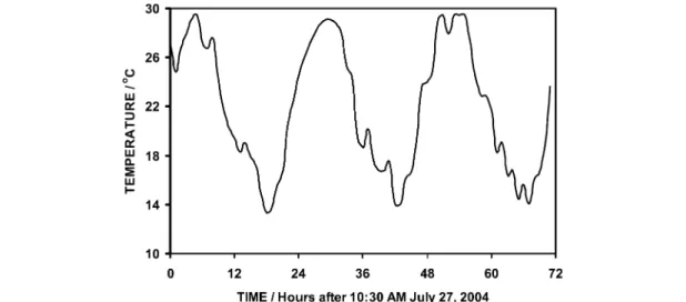
Figure 1 illustrates a pattern of continuously changing temperature as typically experienced by plants in temperate zones. The low for the three days covered in Fig. 1 was 14.1 °C, the high was 29.5 °C, and the mean was 22.0 °C. The 15.4 °C range in temperature is typical of daily temperature variation in in- land temperate zones. An informative way to summarize environmental temperature data is as plots of the time spent at each temperature vs. the temperature, Fig. 2. Such plots show the time that a plant spends at each temperature, and thus the effect of the local temperature variation on growth. Three con- clusions are apparent from this plot. First, mean temperature data clearly do not provide sufficient in- formation for analyzing the relation between temperature and growth of ectotherms. Second, the distri- bution is distinctly bimodal. And third, the time at the mean temperature is small. Plants spend far more time growing at temperatures around 16 and 26 °C than at the mean temperature. Accumulation of data over longer periods, in which average temperatures shift with changing weather patterns and season, leads to plots of temperature distribution that disguise the diurnal temperature shift and appear to be unimodal, but the effects of daily temperature variation on plant growth remain. The widely reported maximum, minimum, and mean temperatures for a day, month, year, etc. are thus a very poor descrip- tion of the temperatures experienced by plants, and correlation of plant growth with these temperature measures can be misleading.

For example, on a global scale, species range and density are correlated with annual mean tem- peratures. However, such correlations do not demonstrate cause and effect relations. This problem is ev- ident in a recent paper by Allen et al. [16], who proposed a cause and effect relation between mean an- nual temperature and the global gradients of species richness based on the linearity of a log-inverse plot, i.e., “the relation between the natural logarithm of species richness and inverse absolute temperature is approximately linear.” They then concluded that the gradient of mean annual temperature with latitudes causes the global gradient of species biodiversity. This conclusion is invalid for at least two reasons.

First, even random data sets are linearized by this type of plot and thus mask the true relationship be- tween variables. Second, mean annual temperature includes both times and temperatures during which growth is not possible, e.g., at 45° latitude, approximately half the year has temperatures that do not allow plant growth, and at 60° most of the temperatures included in the annual mean have no relevance to plant growth. Effects of temperature on plant distributions can only be analyzed in reference to times, seasons, and places when and where plants actually grow.

Fig. 1 Hourly temperatures through 27–29 July 2004 at Logan, UT, USA recorded with a HOBO Pro Series temperature logger from Onset Computer Corp., Bourne, MA.

Fig. 2 Frequency plot (hours per day at each temperature vs. temperature) of environmental temperatures shown in Fig. 1.

The thermally allowed growth season can be defined as the period of time in which most days have several hours above the freezing point of water. This varies from 52 weeks at low elevations near the equator to only 6 to 10 weeks in subpolar and alpine regions. At all elevations and latitudes in the Northern Hemisphere where plant growth is possible, the thermally allowed growth season includes significant portions of the months of June and July. Thus, values of daily maximum and minimum tem- peratures during June and July provide reasonable estimates of temperature and temperature variation during the growth season. Similarly, data for December and January are representative of growth tem- peratures in the Southern Hemisphere.

With these estimates, global patterns of terrestrial growth season temperature and temperature variation can be plotted as averages at each latitude. (This approach neglects the local effects of alti- tude, ocean currents, etc., but allows focus on average, global-scale effects. Altitude will be treated later in the discussion.) Figure 3 presents a plot of maximum high and minimum low temperatures for June and July in the Northern Hemisphere and for December and January in the Southern Hemisphere.

Latitudes near ±30° experience higher temperatures during the growing season than either the tropics or the subpolar regions. Minimum temperatures plateau around the equator and decrease toward the polar regions. For example, plants growing during the Alaskan summer experience higher, as well as lower, temperatures than plants in lowland Costa Rica. Figure 3 also shows the difference between max- imum and minimum temperatures during the growing season (∆T_env). ∆T_envincreases rapidly from the equator to near 35° N latitude, then only slowly to about 70° N. Above 70°, ∆T_envdecreases rapidly. In the Southern Hemisphere, ∆T_envincreases rapidly to nearly 40° S, then decreases. The shape of the

∆T_envcurve suggests that ∆T_envis an important variable determining species distribution. The curve of T_meanvs. latitude is approximately the average of the curves for the maximum and minimum shown in Fig. 3.

TEMPERATURE EFFECTS ON PLANT GROWTH

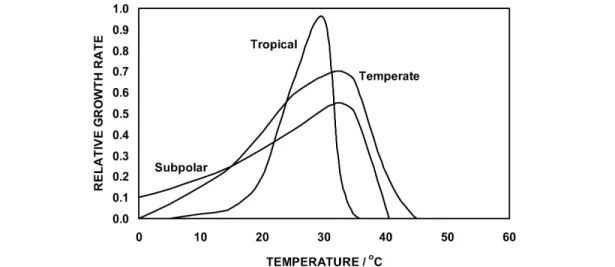
Some typical plant growth rate vs. temperature curves are shown in Fig. 4. Plant growth has high and low temperature limits as well as a (often broad) temperature optimum. Curves in Fig. 4 represent plants adapted to lowland tropics with warm, near constant temperatures, to temperate regions, and to high- latitude or high-elevation locations with very large temperature variations. Such curves, though tedious Fig. 3 Maximum () and minimum (○) temperatures and their difference () for June and July in the Northern Hemisphere and for December and January in the Southern Hemisphere [46].

to obtain by traditional means, can now be rapidly generated for individual plants or populations by calorespirometric measurements of heat and CO₂rates on small, excised bits of growing tissue [19].

Plants well adapted to a site through long periods of natural selection have growth rate vs. tem- perature curves that closely match the temperature distribution plot (e.g., Fig. 2) during the growth sea- son for that site [20–22]. Some plants even exhibit bimodal curves of growth rate vs. temperature that match the bimodal temperature frequency plots of the environment to which they are adapted [21,22].

Closely matched curves indicate a plant is spending much of the time during its growth season near its optimum growth temperature and all of its time within the temperature range allowing growth. Survival, growth, and reproduction of such plants are greatly enhanced relative to plants with temperature optima in a range encountered less often. Plants, of course, only grow at temperatures when other, local environmental variables (such as water and nutrients) are appropriate for the plant.

Relation between respiratory metabolism and growth

As suggested by Hoh and Cord-Ruwisch [23], it is necessary to consider the thermodynamics of growth and temperature responses to develop a correct biological model of the relations between environmen- tal factors and growth and to identify the temperature functions that account for local and global scale distributions. We have developed the required thermodynamic model by expressing growth rate (R_grow) as the product of metabolic rate (measured by the rate of CO₂production, R_CO2) and a function of the substrate carbon conversion efficiency (i.e., the fraction of substrate retained in anabolic products, ε), eq. 1 [1,24].

Growth rate (Cmole s^–1) = R_grow= R_CO2[ε/(1–ε)] (1)

This relation can be derived directly from the equation for respiration-driven growth of plants, C_substrate+ (compounds and ions of N, P, K, etc.) + yO₂→εC_bio+ (1–ε) CO₂ (2) and has been shown to accurately predict relative growth rates of plants from calorespirometric meas- urements [20,25–31]. Both R_CO2 and εare functions of temperature. These temperature responses are such that the R_growfunction in eq. 1 produces the typical skewed bell-curve of R_grow vs. temperature such as those shown in Fig. 4.

Total growth over a season, G, is equal to the integral of eq. 1 over time

Fig. 4 Schematic plots of plant growth rate vs. temperature for plants adapted to near constant tropical temperatures to more variable temperate climate temperatures, and to highly variable subpolar temperatures.

G =

∫

^R_CO2[ε/(1–ε)]dt (3) To establish the link between physiological and temperature variables, eq. 1 must be written in terms of environmental temperature variables. The average rate of CO₂production over the growth season is proportional to the mean kinetic temperature [32], T_MK-CO2, and the efficiency function [ε/(1–ε)] is an inverse function of the temperature variability [33 and see Appendix]. Therefore, approximating T_MK-CO2with T_mean(on the Celsius scale) and temperature variability with ∆T_env, eq. 1 becomes

R_grow= c(T_mean)[f(∆T_env^–1)] (4)

where c is a proportionality constant. Use of the Celsius scale for T_meanassumes that growth rate goes to zero at the freezing point of water; other reference temperatures for zero growth rate could be used as appropriate. And, with the same substitutions as above and with the length of the growth season as

∆t,

G = c(T_mean)[f(∆T_env^–1)]∆t (5)

Equations 4 and 5 establish a relation among growth and the elevation/latitude-dependent parameters;

environmental temperature and growth season. Note that both the growth rate and total growth are pro- portional to the ratio of mean temperature to temperature variability.

Equations 4 and 5 state the law of adaptation of plants to environmental temperatures. The bio- chemical and thermodynamic basis for this law, and thus the reasons for calling it a law are given in the Appendix where the connection between environmental variables and cellular metabolism and thus to genetic adaptation is established.

EXPERIMENTAL TESTS OF THE DERIVED LAW

The above theory predicts plant distributions are related to the ratio of T_meanand an inverse function of

∆T_envduring the growth season. If the theory is correct, these temperature variables determine the res- piratory characteristics of autochthonous plants, the respiratory characteristics determine survival at a given location, and since T_meanand ∆T_envchange systematically with altitude and latitude on a global scale, the environmental temperature determines the distribution of plants on a global scale. This sec- tion reviews some experimental tests of these predictions.

Plant respiratory metabolism varies systematically with altitude and latitude

Criddle et al. [34] examined the Arrhenius temperature coefficients for metabolic heat rate (µ_q) in rap- idly growing tissues of three species of woody shrubs from an approximately 500-km north–south range in the Great Basin region of the United States. Values of µ_qwere a linear function of the altitude and latitude from which the accessions originated. Because the plants tested were grown in a common gar- den, µ_qis clearly a genetically determined adaptation, not an acclimation. Low elevation and low lati- tude accessions had lower temperature coefficients. Also, measurements on over 50 congeneric pairs of other species of perennials showed that the plant from the more northerly latitude or higher elevation always had the smaller temperature coefficient. McCarlie et al. [21] showed subpopulations of cheat- grass (Bromus tectorum) from widespread areas of western North America have large, location-specific differences in temperature responses of metabolic rates, energy efficiency, and growth that match the temperature patterns during growth seasons at the different locations. Studies on eucalyptus from wide- spread locations in Australia yield similar conclusions [26,28,35]. Other studies following simply R_CO2 or R_O2, though giving less well defined spatial dependencies, still show that respiratory properties vary systematically with climate of origin (e.g., [36]). Thus, the evidence is strong that there is a cause and effect relation between the temperature dependence of respiratory rates and the climate of the native ge- ographic locations, which are in turn related to latitude and elevation.

T_mean/^T_envis the environmental temperature function to which plants are adapted Related trees at different elevations

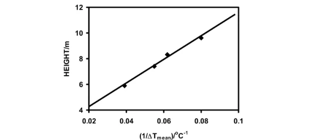
Church [37] tested the predicted inverse relation of growth to ∆T_envwith studies on growth of geneti- cally related trees. Metabolic rate measurements were made on 17 half-sib families of 15-year-old Pinus ponderosa planted at each of four sites with different latitudes and elevations. Although the test sites are at different elevations, the mean temperatures during branch elongation growth are essentially the same at all sites. This results from growth later in the season at higher elevations. Because T_meanis a constant, if growth rates (metabolic rate times efficiency) are proportional to T_mean/∆T_env, relative growth rates at each site are predicted to be proportional to 1/∆T_env. Plots of 1/∆T_envvs. growth rate (as height growth in 15 years) confirm this prediction (Fig. 5). Height decreases linearly with decreasing values of 1/∆T_env(R²= 0.96 for 4 sites with 17 families). Growth rate of these trees is not correlated with any other known environmental variable other than weak correlations with variables that are co- correlated with ∆T_env. This study confirms that ∆T_envis a key environmental variable linking metabo- lism with latitude and elevation. The linear relation between growth and 1/∆T_envalso shows the rela- tion between [ε/(1–ε)] and ∆T_envused in deriving eqs. 4 and 5 is a simple first-order reciprocal.

The treeline boundary

Another test of the hypothesis that growth is proportional to T_mean/∆T_envcan be made using treeline temperature data. If the growth rate or annual growth is constant at treeline irrespective of species, lat- itude and elevation, and if efficiency is directly proportional to the reciprocal of ∆T_env, a plot of T_mean vs. ∆T_envat the treeline is predicted to be a straight line (see eq. 5). Such a plot is shown in Fig. 6. The data produce a remarkably linear relation with the treeline value of ∆T_env/T_meanequal to 2.6. The lin- ear relation again demonstrates the relation between [ε/(1–ε)] and ∆T_envin eqs. 4 and 5 is a simple first- order reciprocal. Note that points added to the plot using T_meanand ∆T_envat locations that are either above or below treeline fall on one or the other side of the line with a rough relation between the dis- tance from the line and distance from treeline (in units of elevation and latitude). The intercept is also essentially zero as required by eq. 5.

Fig. 5 Fifteen-year height growth of ponderosa pine half-siblings planted at four different elevations vs. the reciprocal of the temperature variation at the different sites during branch elongation [37].

Figure 7 shows how treeline elevations vary as a function of latitude in the Northern Hemisphere based on observed treeline elevations [38] and elevations calculated from T_mean, ∆T_env, and latitude data [39]. Agreement between the experimental and calculated curves is remarkably good with the curve for experimental values slightly lower than calculated values. Environmental factors other than temperature may lower treeline elevations from the calculated elevation, but cannot raise them. Therefore, the small difference between the curves is in the correct direction and of reasonable magnitude.

The finding that T_mean/∆T_envis a global constant for treelines generates a hypothesis that the ratio of mean environmental temperature to temperature variability will be a different, but constant, value at each of the boundaries between other life zones [40]. Further, this finding also supports our proposal that T_mean/∆T_envexplains the global-scale gradients in plant species range and density as functions of latitude and altitude.

Fig. 6 Plot of T_meanvs. ∆T_envshowing the zero intercept and linear correlation between these two variables at treeline locations (). Non-treeline sites from equatorial to polar locations are shown by (). Treeline sites: A, Cruz Loma, Ecuador; B, Cotapaxi, Ecuador; C, Nara Moro, Mt. Kenya, Kenya; D, Mt. Wilhelm, Pinduande, New Guinea; E, Cotton Station, CA, USA; F, Dana Meadows, CA, USA; G, Lone Pine, CA, USA; H, Snow Flats, CA, USA; I, Bettles, AK, USA; J, near Ely, NV, USA; K, Bald Mtn., UT, USA. Above treeline sites: w, Gomessiat, Ecuador; x, Mt. Whitney, CA, USA; y, Teleki Valley, Mt. Kenya, Kenya; z, Summit Ridge, Mt. Wilhelm, New Guinea. Below treeline sites: 1, San Francisco, CA, USA; 2, Orange County, CA, USA; 3, upper Provo River Canyon, UT, USA; 4, Feather Falls, CA, USA; 5, Burney, CA, USA; 6, Allegheny, CA, USA; 7, Blue Canyon, CA, USA; 8, Fairbanks, AK, USA; 9, Inskip, CA, USA; 10, Davis, CA, USA. California temperature data are from the California Department of Water Resources database. Utah temperatures were collected in this study. Sources for the remainder are given in ref. [37].

Survival, growth, and reproduction depends on close adaptation of plant metabolism to the pattern of environmental temperatures

Studies on eucalyptus clones and species, sagebrush, and redwood show that small differences in envi- ronmental temperature selectively favor growth of one plant over another as predicted by the law of temperature adaptation.

Eucalyptus clones

Large plantings of two closely related, rapid-growing clones of Eucalyptus camadulensis in an irrigated, well-managed, common garden in the Central Valley of California differed in growth from year to year.

Calculations of growth rate vs. temperature based on calorespirometry measurements showed Simpson Timber Co. clone 4016 had a relatively narrow curve for growth rate vs. temperature with an optimum near 25 °C. Clone C11 had a broader curve with its optimum near 30 °C. Clone 4016 was calculated to be more efficient over a narrow range of temperatures. Clone C11, while less efficient over most of the temperature range, was predicted to be more efficient than 4016 at higher temperatures. These predic- tions were borne out by annual growth measurements. Clone C11 consistently outgrew clone 4016 dur- ing warmer years, yet was the slower of the two during cooler years. Total growth of the two clones over seven years was nearly equal. The different growth responses to temperature of these two clones were predicted by differences in responses of metabolic rate and efficiency to temperature [26].

Sagebrush

Two subspecies of sagebrush (Artemisia tridentata Nutt. ssp. tridentata Nutt. and A. tridentata Nutt.

ssp. vaseyana [Rydb.] Beetle) and a stable hybrid swarm lying between the two occur naturally over an elevation gradient of only 85 m and a distance of only 1.1 km on an east-facing hillside near Nephi, Utah [41]. Three common gardens were established at the bottom, middle, and top of the site to test dif- ferences giving rise to this distribution. Plants in the three gardens and others recruited from proximal areas were reciprocally transplanted both lower and higher on the hillside. Transplanted plants fail to thrive and often die after one or two seasons. Though soil composition differed among sites, moving soil along with plants from one garden to another had no effect on these outcomes. The sites have been exhaustively analyzed for differences in herbivory, water, soil microbes, etc. with no significant differ- ence found except in environmental temperature [42]. Temperature differences were small, but signifi- Fig. 7 Comparison of calculated () and measured (–) [38] treeline elevations as a function of latitude.

cant [43,44]. Differences occur in both mean temperatures and temperature variability. Corresponding differences in metabolic responses to temperature were found among the sagebrush subspecies and hy- brids [43]. The results are consistent with the hypothesis that very small differences in temperature de- pendence of respiration can dictate success or failure of a subspecies or hybrid population and thereby determine their locations for successful growth.

Redwood growth and distribution

California coast redwoods (Sequoia sempervirens) have been studied extensively to establish relation- ships among respiration, growth rate, range, and temperature. The geographic origins of redwood seedlings collected from the length of the native range along the California and Oregon coasts (but grown in a common greenhouse) can be determined from measurements of the temperature dependence of the respiratory heat rate [25,45]. Trees from the more northern and more variable temperature end of the range have smaller temperature coefficients and are therefore less affected by temperature variabil- ity. Each population appears to be genetically adapted to the temperature pattern of its native climate.

Such variation in genetically defined properties of metabolism allows a species range much greater than the allowed range of growth for a plant or population within the species.

Eucalyptus species studies

The relation predicted to exist among climate, respiration, and distribution has also been tested with Eucalyptus species (Fig. 8) (and other species [20]) from native climates with different T_meanand ∆T_env. Figure 8 shows plots of normalized growth rate (as ∆H_BR_grow) calculated from measured respiration properties vs. temperature for individual trees of three Eucalyptus species. All were grown in, and there- fore acclimated to, a common environment. The responses of the species to temperature and also the growth temperature ranges for the three species differ. The growth temperature ranges are consistent with the high and low temperatures at the native locations as indicated at the bottom of Fig. 8. This fig- ure also makes the point that metabolism must be adapted to the absolute values of the extremes of the temperature range. Intra-species variation occurs among plants of each of these species, but intra- species differences are smaller than between species differences, making curves in Fig. 8 for individual plants good approximations of each species as a whole.

The experimental evidence presented above, and much more that is not discussed here, confirms that plants are adapted to the temperature function, T_mean/∆T_env, and shows that plants within each habi- tat are closely adapted to the microclimate of that habitat. For example, the data on ponderosa pine growth and treeline temperatures show the appropriate temperature function describing plant growth is a direct proportionality to T_meanand an inverse proportionality to the first power of ∆T_env. Also, data of the type in Fig. 8 on many species show that the high and low thresholds for growth of autochthonous plants match the maximum and minimum temperatures of the environment during the growth season.

The next section shows quantitatively how T_mean/∆T_envis related to altitude and latitude and thus leads to altitudinal and latitudinal gradients of species range and density.

LATITUDINAL TRENDS IN T_mean/^T_env^{AND T}_env^/T_mean

Figure 9 shows latitudinal patterns in T_mean/∆T_envand ∆T_env/T_meanderived from climate data [46]. The curves are normalized to have T_mean/∆T_envvalues of 1.0 at the equator. ∆T_env/T_meanis small at low lat- itude and large at high latitude, similar to species ranges. Values of the inverse ratio, T_mean/∆T_env, de- crease slowly with increasing latitude in tropical regions, more rapidly near the edge of the tropical zone (about +24° and –15° latitude), then again more slowly to near the polar zones, similar to species den- sities.

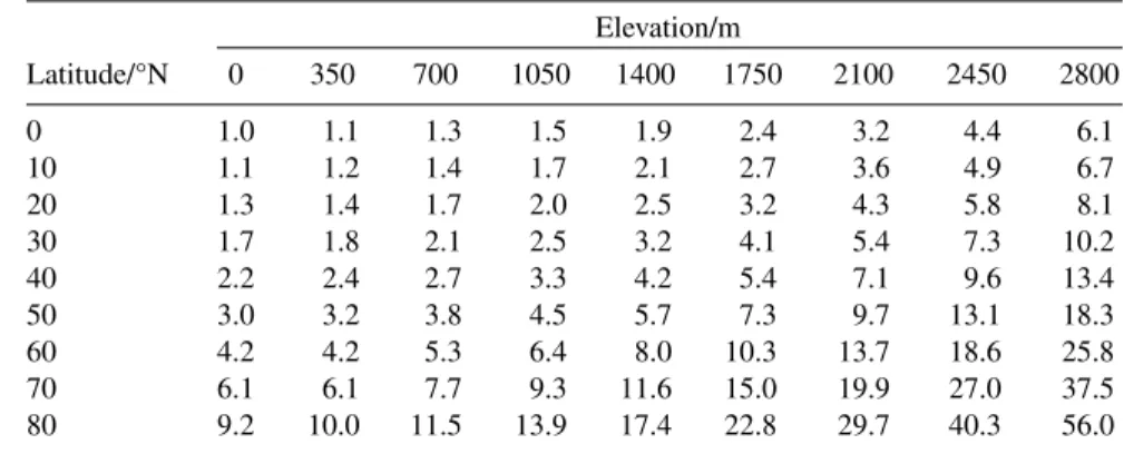
Deviations from the average, global, latitudinal trends in these ratios exist owing to local geo- graphical features such as mountains, proximity to oceans, etc. For example, mountainous locations cause wrinkles in the global contour maps of ∆T_env/T_meanand T_mean/∆T_env. The empirical “rule-of- thumb” that a 1° increase in latitude is approximately equivalent to 35-m increase in elevation in its ef- fects on temperature can be used to estimate the size of the wrinkles. Table 1 shows the estimated, rel- ative values of ∆T_env/T_meanin the Northern Hemisphere as both latitude and elevation change. Table 2 shows relative values of T_mean/∆T_envas functions of both latitude and elevation.

Fig. 8 Normalized rates of growth (as ∆H_BR_grow, where ∆H_Bis the difference in the heats of combustion of carbohydrate and biomass) for three eucalyptus species (Eucalyptus globulus Labill, E. grandis W. Hill ex Maiden, E. saligna Sm.). Values were calculated from measurements of respiratory heat and CO₂ production rates as a function of temperature. The environmental temperature range for growth of the species is given at the bottom of the figure.

Table 1 The ratio, ∆T_env/T_mean, as a function of latitude and elevation, calculated assuming 1° of latitude is equivalent to 35 m of elevation and normalized to unity at sea level at the equator.

Elevation/m

Latitude/°N 0 350 700 1050 1400 1750 2100 2450 2800

0 1.0 1.1 1.3 1.5 1.9 2.4 3.2 4.4 6.1

10 1.1 1.2 1.4 1.7 2.1 2.7 3.6 4.9 6.7

20 1.3 1.4 1.7 2.0 2.5 3.2 4.3 5.8 8.1

30 1.7 1.8 2.1 2.5 3.2 4.1 5.4 7.3 10.2

40 2.2 2.4 2.7 3.3 4.2 5.4 7.1 9.6 13.4

50 3.0 3.2 3.8 4.5 5.7 7.3 9.7 13.1 18.3

60 4.2 4.2 5.3 6.4 8.0 10.3 13.7 18.6 25.8

70 6.1 6.1 7.7 9.3 11.6 15.0 19.9 27.0 37.5

80 9.2 10.0 11.5 13.9 17.4 22.8 29.7 40.3 56.0

Table 2 The ratio, T_mean/∆T_env, as a function of latitude and elevation, calculated assuming 1° of latitude is equivalent to 35 m of elevation and normalized to unity at sea level at the equator.

Elevation/m

Latitude/°N 0 350 700 1050 1400 1750 2100 2450 2800

0 1.00 0.92 0.80 0.66 0.53 0.41 0.31 0.23 0.16

10 0.91 0.84 0.72 0.60 0.48 0.37 0.28 0.21 0.15

20 0.76 0.70 0.60 0.50 0.40 0.31 0.23 0.17 0.12

30 0.60 0.55 0.48 0.40 0.32 0.25 0.19 0.14 0.10

40 0.46 0.42 0.36 0.30 0.24 0.19 0.14 0.10 0.07

50 0.33 0.31 0.27 0.22 0.18 0.14 0.10 0.08 0.05

60 0.24 0.24 0.19 0.16 0.12 0.10 0.07 0.05 0.04

70 0.16 0.16 0.13 0.11 0.09 0.07 0.05 0.04 0.03

80 0.11 0.10 0.09 0.07 0.06 0.04 0.03 0.02 0.02

Fig. 9 T_mean/∆T_env(^{) and ∆T}env/T_mean() as functions of latitude. Positive latitude values indicate north and negative values south.

PATTERNS OF SPECIES DENSITY AND SPECIES RANGE ARISE FROM GRADIENTS IN T_mean/^T_env^{AND T}_env^/T_mean, RESPECTIVELY

As further explained in the Appendix, responses of physiological processes to environmental tempera- tures determine where a plant can grow. Natural selection leads to plants with an optimized product of respiration rate and efficiency and a growth temperature range that matches the range of environmental temperatures during the growth season. The nonequilibrium thermodynamic arguments in the Appendix show that plants can increase energy use efficiency by adaptation of energy metabolism to a narrowed range of environmental temperatures. However, this presents risk of death from loss of metabolic con- trol during temperature events outside the range of adaptation [47–49]. In contrast, adaptation to a broader temperature range enhances the ability to survive at temperature extremes, but at the expense of reduced efficiency and therefore the ability to compete. Thus, natural selection balances these two adaptive forces, leading to plants with a growth curve that closely matches the local environmental tem- perature distribution.

The temperature adaptation law expressed in eqs. 4 and 5 together with natural selection by en- vironmental temperature leads to the global pattern of species distribution [50]. Extension of Fig. 6, i.e., roughly a quadrangle formed by the treeline line shown and lines bounding areas on earth where plants grow, delimits the area (in T–∆T coordinates) that allows growth. The areas in this quadrangle defined by populations of plants metabolically adapted to the same ∆T_envand T_meanare variable. The size of the area is thus determined by the magnitude of the temperature range of the environment, ∆T_env(see Fig 8). ∆T_env equals both the temperature range of the environment and the temperature range for growth of a population of well-adapted plants (see Fig. 8, ref. [20], and the above paragraph). ∆T_envis thus the variable metric of population or species range in T–∆T coordinates. In T–∆T coordinates, pop- ulation (or species) area increases from the tropics to the poles, and because ∆T_envalso increases from the tropics to the poles, the observed geographic, global gradients of species density and range arise from the latitudinal dependence of the ratios, T_mean/∆T_envand ∆T_env/T_mean, respectively. These conclu- sions apply, regardless of the uncertainty in the definition of what constitutes a biological unit, e.g., pop- ulation, subspecies, species, families or even ecosystems. As long as the definition is consistent, the

∆T_envmetric can be applied to populations, subspecies, species or other taxonomic groups.

Assuming the relations between species range and ∆T_env/T_meanand between species density and T_mean/∆T_envare linear, then species density, defined as the number of species per unit area, is

species density = N/A = c'(T_mean/∆T_env) (6)

where N is the total number of species in area A and c' is a proportionality constant that depends on the taxon definition. Since the average species range is the area divided by the number of species in that area,

species range = A/N = c"(∆T_env/T_mean) (7)

Equations 6 and 7 predict curves of species range and density with latitude and are proportional to the curves in Fig. 9.

Adjustment for effects of area on species density

Before the predictions of eqs. 6 and 7 can be compared with observed trends, the predicted results may need to be corrected for the effect of variation of land area with latitude. The effect of land area may al- ready be included in the temperature data shown in Fig. 9 because larger land areas include a wider range of values of T_mean/∆T_envat a given latitude. But, assuming the effects of temperature and land area are independent, corrections can be estimated from land area as a function of latitude.

According to the general species-area relationship [2,14,17],

N = kA^z (8)

Values of z from 0.1 to 0.6 have been reported [17,51] with most commonly reported z values near 0.4 [12]. Figure 10 shows land areas as a function of latitude normalized to the area at the equator. Values from Fig. 10 were then used to calculate species density vs. latitude plots using eq. 8 with z = 0.4 (Fig. 11, open symbols). These curves show that land area has little effect on the overall global patterns of latitudinal gradients of species density and range. Changes in z from 0.2 to 0.6 have small effects, re- ducing or increasing, respectively, the difference between the temperature-based curves of species den- sity and the area-corrected curve.

Fig. 10 Land area as a function of latitude from measurements of the combined lengths of land segments along latitudinal lines at 5° intervals. Northern Hemisphere latitudes are shown as (+) degrees and Southern Hemisphere latitudes as (–). See also [17], p. 285.

Fig. 11 Calculated average species density without () and with (○) correction for land area, plotted against latitude in the Northern (+) and Southern (–) Hemispheres. Values are normalized to give a value of 1.0 at the equator.

Comparison of predicted range and density with observations

The variation in species range and density predicted by Figs. 9 and 11 are in general agreement with di- rect observations of latitudinal changes in species range and density. For example, the prediction of a near two-fold decrease in species density from 12° to 45° north latitude indicated by Fig. 11 is close to reported values [9]. These results give general support to the equations derived above. The predictions of species range and density made with eqs. 6–8 are relative values. To apply the model to calculate real numbers for species densities and ranges, calibration constants using observed species numbers at many locations will be required. Such data on species numbers will also provide critical tests of the theory.

Obtaining these, however, will not be easy. Among the problems is uncertainty in definitions of species and questions of whether the theory should more appropriately be framed in terms of other taxa.

CONCLUSIONS

The thermodynamic arguments presented here are generated from fundamental physical and physio- logical principles considering the thermodynamic effects of temperature and temperature variability on ectotherm energy use efficiency and metabolic rate, and therefore on productivity, as explained in the Appendix. Because the derivation is based on first principles, we refer to eqs. 4 and 5 as the law of tem- perature adaptation. This law applies universally to growth and distribution of ectotherms, and defines temperature conditions in which growth of a given organism can, but not necessarily will, occur.

Ecologists have long asked “Are there general laws in ecology?” [52]. This paper defines such a law of ecology with a firm basis in thermodynamics and biochemistry.

The responses of physiological variables to temperature account for only one factor limiting ectotherm distribution. We recognize that modulators such as predation, symbionts, habitat variability, historical development, and scarcity of necessary resources (e.g., water or minerals) can prevent growth at any given location irrespective of favorable temperature conditions [14,53]. However, the law of temperature adaptation defines relative species range and density from fundamental thermo- dynamic principles, physiology of energy metabolism, and global patterns of climate that are in- escapably superimposed on all local and historical determinants of the existence of a species at a par- ticular location.

A perfect adaptation of plants to temperature is not possible because climate at any site varies from year to year. There is, thus, no single “best” solution for adaptation of energy metabolism and growth rate to a location. Organisms (both within and between species) with a range of properties exist at all sites, some better at growth and overcoming competition, others better at survival through climatic extremes. The weather “tomorrow” determines which is more fit. The relation between metabolic prop- erties and location is further complicated because plants may also alter their effective environmental growth temperatures simply by altering the time during the season when growth occurs. Such responses add a “fuzziness” to the patterns of species range and density, but in all cases, growth remains subject to the limitations imposed by T_meanand ∆T_envat the time of growth.

While answering important how and why questions of global gradients of species range and den- sity, the law of temperature adaptation also provides a theoretical basis to correct for elevation differ- ences, temperature-moderated regions, etc., locally altering the global pattern. The law of temperature adaptation, together with physiological measurements, can be employed to predict relative productivity of cultivars when used for agriculture or forestry in a particular climate, or to determine a most suitable climate for optimum productivity [54]. One only need measure (or for managed environments, set) the temperature distribution curve for a site during the growing season and the growth rate vs. temperature curve for the genotype. The more closely these two curves match, the more productive the genotype will be in the environment at the site. Integration of the growth rate curve over the temperature distribution during the growth season allows quantitative comparison of growth of different genotypes. If our hy- pothesis is correct that the ratio of mean temperature to temperature variability is constant at boundaries

between life zones, it could be used to predict how climate change will affect the distribution of ecto- therms.

REFERENCES

1. L. D. Hansen, C. Macfarlane, N. McKinnon, B. N. Smith, R. S. Criddle. Thermochim. Acta 422, 55–61 (2004).

2. C. B. Wilson. Nature 152, 264–267 (1943).

3. P. H. Klopfer. Am. Naturalist 94, 337–342 (1959).

4. A. G. Fisher. Evolution 14, 64–81 (1960).

5. F. G. Stehli, R. G. Douglas, N. D. Newell. Science (AAAS) 164, 947–949 (1969).

6. M. Huston. Am. Naturalist 113, 81–101 (1979).

7. J. H. Brown. Am. Naturalist 124, 255–279 (1984).

8. G. C. Stevens. Am. Naturalist 140, 893–911 (1989).

9. K. Rohde. Oikos 65, 514–527 (1992).

10. A. Hallam. An Outline of Phanerozoic Biogeography, Oxford University Press, New York (1994).

11. E. R. Pianka. Am. Naturalist 100, 33–46 (1996).

12. I. Hanski and M. Gyllenberg. Science (AAAS) 275, 397–400 (1997).

13. K. Rohde. Oikos 79, 169–172 (1997).

14. K. Rohde. Ecography 22, 593–613 (1999).

15. K. J. Gaston. Oikos 84, 309–312 (1999).

16. A. P. Allen, J. H. Brown, J. F. Gillooly. Science (AAAS) 297, 1545–1548 (2002).

17. M. L. Rosenzweig. Species Diversity in Space and Time, Cambridge University Press, Cambridge (1995).

18. T. J. Davies, V. Savolainen, M. W. Chase, J. Moat, T. G. Barraclough. Proc. R. Soc. London, Ser.

B 271, 2195–2200 (2004).

19. R. S. Criddle and L. D. Hansen. In Handbook of Thermal Analysis and Calorimetry, Vol. 4, From Macromolecules to Man, R. D. Kemp (Ed.), pp. 711–763, Elsevier, Amsterdam (1999).

20. R. S. Criddle, B. N. Smith, L. D. Hansen. Planta 201, 441–445 (1997).

21. V. W. McCarlie, L. D. Hansen, B. N. Smith, S. B. Monsen, D. J. Ellingson. Russ. J. Plant Physiol.

50, 183–191 (2003).

22. L. D. Hansen, J. N. Church, S. Matheson, V. W. McCarlie, T. Thygerson, R. S. Criddle, B. N.

Smith. Thermochim. Acta 388, 415–425 (2002).

23. C-Y. Hoh and R. Cord-Ruwisch. Water Sci. Technol. 36, 109–115 (1997).

24. L. D. Hansen, M. S. Hopkin, D. R. Rank, T. S. Anekonda, R. W. Breidenbach, R. S. Criddle.

Planta 194, 77–85 (1994).

25. T. S. Anekonda, R. S. Criddle, W. J. Libby, R. W. Breidenbach, L. D. Hansen. Plant Cell Environ.

17, 197–203 (1994).

26. T. S. Anekonda, L. D. Hansen, M. Bacca, R. S. Criddle. Can. J. For. Res. 26, 1556–1568 (1996).

27. R. S. Criddle, T. S. Anekonda, R. M. Sachs, R. W. Breidenbach, L. D. Hansen. Can. J. For. Res.

26, 1569–1576 (1996).

28. R. S. Criddle, T. S. Anekonda, S. Tong, J. N. Church, F. T. Ledig, L. D. Hansen. Aust. J. Plant Physiol. 27, 435–443 (2000).

29. D. K. Taylor, D. R. Rank, D. R. Keiser, B. N. Smith, R. S. Criddle, L. D. Hansen. Plant Cell Environ. 21, 1143–1151 (1998).

30. N. E. Marcar, R. S. Criddle, J. M. Guo, Y. Zohar. Functional Plant Biol. 29, 925–932 (2002).

31. C. Macfarlane, M. A. Adams, L. D. Hansen. Proc. R. Soc. London, Ser. B 269, 1499–1507 (2002).

32. R. M. Schoolfield, P. J. H. Sharpe, C. E. Magnuson. J. Theor. Biol. 88, 719–731 (1981).

33. G. Nicolis and I. Prigogine. Self-Organization in Nonequilibrium Systems, John Wiley, New York (1977).

34. R. S. Criddle, M. Hopkins, E. D. McArthur, L. D. Hansen. Plant Cell Environ. 17, 233–243 (1994).

35. T. S. Anekonda, R. S. Criddle, M. J. Bacca, L. D. Hansen. Functional Ecol. 13, 675–682 (1999).

36. M. J. Earnshaw. Arctic Alpine Res. 13, 425–430 (1981).

37. J. N. Church. Tests of the ability of a respiration based growth model to predict growth rates and adaptation to specific temperature conditions: Studies on Pinus ponderosa and Eucalyptus species. Ph.D. dissertation. University of California at Davis (2001).

38. C. Körner. Alpine Plant Life, Functional Plant Ecology of High Mountain Ecosystems, Springer Verlag, Berlin (1999).

39. M. New, M. Hulme, P. Jones. J. Climate 12, 829–856 (1999).

40. C. H. Merriam. National Geographic Magazine 6, 229–238 (1894).

41. D. C. Freeman, W. A. Turner, E. D. McArthur, J. H. Graham. Am. J. Bot. 78, 805–815 (1991).

42. K. J. Miglia, D. C. Freeman, E. D. McArthur, B. N. Smith. Importance of genotype, soil type, and location on the performance of parental and hybrid big sagebrush reciprocal transplants in the gar- dens of Salt Creek Canyon. USDA Forest Service Proceedings RMRS-P-31, pp. 30–36 (2004).

43. B. N. Smith, S. Eldrige, D. L. Moulton, T. A. Monaco, A. R. Jones, L. D. Hansen, E. D.

McArthur, D. C. Freeman. Differences in temperature dependence of respiration distinguish sub- species and hybrid populations of big sagebrush: nature vs. nurture. USDA Forest Service Proceedings RMRS-P-11, pp. 25–28 (1999).

44. B. N. Smith, T. A. Monaco, C. Jones, R. A. Holmes, L. D. Hansen, E. D. McArthur, D. C.

Freeman. Thermochim. Acta 394, 205–210 (2002).

45. T. S. Anekonda, R. S. Criddle, W. J. Libby. Can J. For. Res. 24, 380–389 (1994).

46. E. A. Pearce and C. G. Smith. The World Weather Guide, Hutchinson, London (1984).

47. R. H. Whittaker. Communities and Ecosystems, p. 30, Macmillan, New York (1970).

48. P. Stiling. Introductory Ecology, pp. 198–200, Prentice Hall, Englewood Cliffs, NJ (1992).

49. P. Stiling. Ecology, Theories and Applications, Prentice Hall, Englewood Cliffs, NJ (1996).

50. R. S. Criddle, J. N. Church, B. N. Smith, L. D. Hansen. Russ. J. Plant Physiol. 50, 192–199 (2003).

51. M. L. Rosenzweig. In: Biodiversity Dynamics, Turnover of Populations, Taxa, and Communities, M. L. McKinney and J. A. Drake (Eds.), pp. 311–348, Columbia Univ. Press, New York (1998).

52. J. H. Lawton. Oikos 84, 177–192 (1999).

53. R. H. Fraser and D. J. Currie. Am. Naturalist 148, 138–159 (1996).

54. L. D. Hansen, B. N. Smith, R. S. Criddle. Pure Appl. Chem. 70, 687–694 (1998).

55. D. Jou and J. E. Llebot. Introduction to the Thermodynamics of Biological Processes, pp. 49–51, Prentice Hall, Englewood Cliffs, NJ (1990).

56. R. B. Kemp. In Principles of Medical Biology, Vol. 4, Cell Chemistry and Physiology: Part III, pp. 303–329, JAI Press, London (1996).

57. R. B. Kemp and Y. Guan. Thermochim. Acta 300, 199–211 (1997).

58. J. Wrigglesworth. Energy and Life, Taylor and Francis, London (1997).

59. J. W. Stucki. Eur. J. Biochem. 109, 269–283 (1980).

60. D. E. Atkinson. Cellular Energy Metabolism and Its Regulation in Metabolism, John Wiley, New York (1977).

61. J. W. Stucki. In Metabolic Compartmentation, H. Seis (Ed.), pp. 39–69, Academic Press, New York (1989).

62. J. W. Stucki. Adv. Chem. Phys. 55, 141–167 (1984).

63. L. D. Hansen, B. N. Smith, R. S. Criddle, J. N. Church. Responses of plant growth and metabo- lism to environmental variables predicted from laboratory measurements. USDA Forest Service Proceedings RMRS-P-00, pp. 1–6 (2001).

64. A. L. Moore, M. S. Albury, P. G. Crichton, C. Affourtit. Trends Plant Sci. 7, 478–481 (2002).

65. O. Kedem and S. R. Kaplan. Trans. Faraday Soc. 61, 1897–1911 (1965).

66. H. V. Westerhoff and K. van Dam. Thermodynamics and Control of Biological Free-energy Transduction, Elsevier, Amsterdam (1987).

67. O. F. Ksenzhek and A. G. Volkov. Plant Energetics, pp. 128–131, Academic Press, New York (1998).

68. S. Nath. Pure Appl. Chem. 70, 639–644 (1998).

69. I. Zotin. Thermodynamic Bases of Biological Processes: Physiological Reactions and Adaptations, pp. 27–41, De Gruyter, Berlin (1990).

70. M. Lewis and M. Randall. Thermodynamics 2^nded., revised by K. S. Pitzer and L. Brewer, p. 100, McGraw-Hill, New York (1961).

APPENDIX: BIOMECHANICAL AND THERMODYNAMIC BASES FOR THE LAW OF ADAPTATION TO ENVIRONMENTAL TEMPERATURES

Relation between efficiency (e) and temperature variability

Definition of the relations between plant metabolism and distribution (elevation/latitude) and tempera- ture requires understanding the relation between the substrate carbon conversion efficiency, ε, and tem- perature. The assumption that εdecreases with increasing temperature variation (i.e., that [ε/(1–ε)] is an inverse function of ∆T) is validated by the second law of thermodynamics, which requires that mass and energy flow through the system described by eq. 2 must be accompanied by heat transfer from the system to the surroundings [55–58]. The relation between the magnitude of the heat loss per unit of bio- mass produced and variability of conditions is given by the theorem of minimal entropy production at steady state [33]. This theorem states that, for any reaction sequence, the steady state is characterized by a minimum rate of entropy production. Any displacement from steady state, i.e., variable reaction conditions such as ∆T_env, results in an increased energy loss to the environment for a given amount of reaction.

The requirement for εto vary with variable conditions can also be understood from consideration of the biochemistry of respiration. Plant growth requires respiration of a fraction of the products from photosynthesis to produce CO₂and energetic intermediates (largely ATP and NADH) that are subse- quently used in anabolic reactions for conversion of additional substrate into plant biomass. The over- all reaction for aerobic growth of plants (eq. 2) is thus the sum of the catabolic reaction

C_substrate+ yO₂+ nADP + nPi + aNAD⁺→CO₂+ nATP + aNADH + aH⁺ (9) and the anabolic reaction

C_substrate+ x(compounds and ions of N, P, K, etc.) + mATP + bNADH + bH⁺→

C_bio+ mADP + mPi + bNAD⁺ (10)

For plants, C_substratein these equations represents photosynthate (carbohydrate) and C_biois used to in- dicate all carbon in anabolic products.

Reactions 9 and 10 occur in the condition-dependent ratio (1–ε)/ε. The two reactions are energy- coupled through cyclic production and hydrolysis of ATP and redox cycling of NADH. However, they are not stoichiometrically coupled [59]. Because the rates of reactions 9 and 10 have different depend- encies on temperature and other reaction conditions, the pairs of coefficients n and m, and a and b, re- spectively for the two reactions, are generally not equal and vary with conditions, i.e., there is variable stoichiometry between anabolism and catabolism. As a consequence, substrate carbon conversion effi- ciency varies with temperature and other changing reaction conditions.

Requirement for maintaining near constant phosphorylation potential while evaries, the role of futile cycles

Unequal and changing relative rates of reactions 9 and 10 for formation and use of ATP and NADH as reaction conditions change cannot be allowed to significantly alter [ATP]/[ADP] ratios because survival of all active organisms requires cellular redox and phosphorylation potentials (or free energy change for hydrolysis of ATP) to remain in a narrow range [58–62]. Maintaining ATP/ADP ratios in varying tem- perature conditions is a major problem because adenine nucleotide concentrations in the cell are only millimolar, while turnover of ATP is very rapid. One gram of meristematic tissue of actively growing plants produces (and hydrolyzes) approximately 1 g of ATP each day. Loss of control of the phospho- rylation potential when temperatures exceed the range to which the plant is adapted lead to chilling or heat shock responses such as loss of membrane integrity and electrolyte leakage [20].

To maintain the cellular phosphorylation potential nearly constant, reaction 9 must always pro- duce ATP and NADH at rates equal to or in excess of their rates of use in the biosynthetic reactions of

reaction 10 (i.e., n≥m and a≥b). If ATP is synthesized slower than it is used, the phosphorylation po- tential falls (degree of coupling decreases) and cell death eventually would ensue. If ATP is synthesized faster than it is used for biosynthesis, the excess can be disposed of by hydrolytic reactions. The bal- ance between the rates of ATP synthesis and use is maintained by condition-dependent “futile” uncou- pled hydrolysis of ATP or equally “futile” reactions that decrease the rate of ATP synthesis by short- circuiting electron transport [22,63,64]. The overall result is a condition-dependent energy loss, a variable coupling between catabolic and anabolic processes, and a condition-dependent ratio of energy loss to growth. Plants adapted to, and growing in, climates with large variations in reaction conditions must “waste” more energy to maintain phosphorylation potentials over a wider range than narrowly adapted plants. Thus, the larger ∆T_env, the lower the energy use efficiency.

A thermodynamic requirement for the engagement of futile pathways for optimizing coupling of substrate oxidation and phosphorylation in changing reaction conditions has been demonstrated from considerations of linear nonequilibrium thermodynamics [55,65–67]. Stucki [61] provided evidence that it is correct to apply the theorem of minimal entropy production to steady state oxidative phospho- rylation (also see [68]) and demonstrated linear force-flow relations in oxidative phosphorylation in mi- tochondria. Various workers [54,68] have confirmed that these concepts also apply generally to growth of cells under near steady-state conditions and have used measurements of heat dissipated as an indi- cation of the increase in entropy during variable growth conditions. They showed that variation in re- action conditions around steady state or a displacement to a higher steady-state rate results in increased heat loss per unit of biomass produced. Thermodynamic arguments thus require, and experimental stud- ies show, that efficiency decreases as ∆T_envincreases. To maintain phosphorylation potentials, ATP syn- thesis must be partially uncoupled or some ATP must be hydrolyzed without coupling to anabolic re- actions. The amount of “wasted” ATP must be coordinated with the changes in environmental conditions to ensure equality of the overall rates of synthesis and hydrolysis of ATP. The condition-de- pendent waste of ATP reduces the substrate carbon conversion efficiency, but thereby maintains cell vi- ability. Several sources infer (but do not rigorously prove for biological systems) that the larger and more frequent the variations perturbing steady state growth, the greater the energy loss from the system [69,70].