Tracking the Gaze on Objects in 3D How do People Really Look at the Bunny? XI WANG,

presented in varying viewing conditions and made of different materials. Our experimental setup is carefully designed to allow for accurate calibration and measurement. We estimate a mapping from the pair of pupil positions to 3D coordinates in space and register the presented shape with the eye tracking setup. By modeling the fixated positions on 3D shapes as a probability distribution, we analysis the similarities among different conditions. The resulting data indicates that salient features depend on the viewing direction.

Stable features across different viewing directions seem to be connected to semantically meaningful parts. We also show that it is possible to estimate the gaze density maps from view dependent data. The dataset provides the necessary ground truth data for computational models of human perception in 3D.

CCS Concepts: •Computing methodologies→Shape analysis; Additional Key Words and Phrases: eye tracking, mesh saliency, 3D object viewing

ACM Reference Format:

Xi Wang, Sebastian Koch, Kenneth Holmqvist, and Marc Alexa. 2018. Track- ing the Gaze on Objects in 3D: How do People Really Look at the Bunny?.

ACM Trans. Graph.37, 6, Article 188 (November 2018), 18 pages. https:

//doi.org/10.1145/3272127.3275094

1 INTRODUCTION

A large part of geometry processing in computer graphics is based on perceptually-based metrics [Lavoué and Corsini 2010] and visu- ally salient shape features [Lee et al. 2005; Song et al. 2014a]. Salient features are usually defined as objects or regions that draw atten- tion of human observers. Interestingly, most approaches are based entirely on geometric or information theoretic measures. Those that are based on experiments almost exclusively use renderings of the shapes presented on a screen for evaluation (e.g. [Bulbul et al.

2011; Dutagaci et al. 2012; Feixas et al. 2009; Kim et al. 2010]). We

Authors’ addresses: Xi Wang, TU Berlin, Department of Computer Science and Electrical Engineering, Sekretariat MAR 6-6, Marchstr. 23, Berlin, 10587, Germany, xi.wang@tu- berlin.de; Sebastian Koch, TU Berlin, Department of Computer Science and Electrical Engineering, Sekretariat MAR 6-6, Marchstr. 23, Berlin, 10587, Germany, s.koch@tu- berlin.de; Kenneth Holmqvist, Universität Regensburg, Institute für Psy- chologie, Universitätsstrasse 31, Regensburg, 93053, Germany, kenneth.holmqvist@ur.

de; Marc Alexa, TU Berlin, Department of Computer Science and Electrical Engineering, Sekretariat MAR 6-6, Marchstr. 23, Berlin, 10587, Germany, marc.alexa@tu- berlin.de.

Permission to make digital or hard copies of all or part of this work for personal or classroom use is granted without fee provided that copies are not made or distributed for profit or commercial advantage and that copies bear this notice and the full citation on the first page. Copyrights for components of this work owned by others than ACM must be honored. Abstracting with credit is permitted. To copy otherwise, or republish, to post on servers or to redistribute to lists, requires prior specific permission and /or a fee. Request permissions from permissions@acm.org.

© 2018 Association for Computing Machinery.

0730-0301/2018/11-ART188 $15.00 https://doi.org/10.1145/3272127.3275094

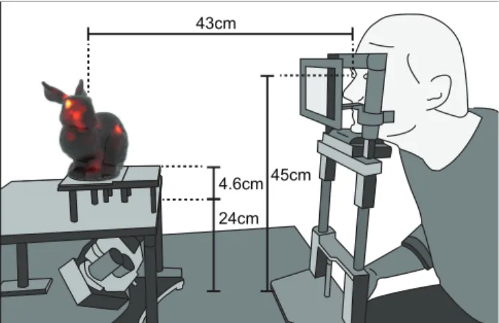
43cm

24cm 4.6cm 45cm

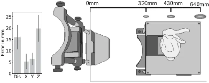
Fig. 1. Schematic of the experimental setup. Shapes are placed approxi- mated100mm below the eyes.

find that data derived from human observers inspecting physical manifestations of 3D shapes would provide a firmer ground for com- putational models of human perception. In this paper we present an experimental setup for this task and gather data from over 70 participants on 16 shapes presented in 14 conditions.

The original notion of salient visual features derives from eye tracking experiments using images presented on a screen as visual stimuli. The main idea is that humans tend to attend to the most important parts of a scene first (see more on this argument in Sec- tion 2). Computational models of saliency [Itti and Koch 2001] were developed only after some consensus had been reached on the local image characteristics that seemed to evoke attention.

Presenting the stimulus on a screen leads to a simple experimental

setup. It has been argued [Kowler 2011] that only the visual percept

on the retina matters, so restricting stimuli to images might suffice

to learn about saliency of features. This point of view is questioned

more and more [Henderson et al. 2007; Itti and Borji 2015; Tatler

et al. 2011]. If 3D shapes are restricted to virtual environments, such

as being only presented on screens, then screen-based experiments

naturally provide the necessary insight. And while it may be true

that computer graphics researchers rather deal with teapots and

bunnies on-screen, 3D computer graphics and, more specifically, ge-

ometry processing derive their importance from the fact 3D shapes

describe the “real world”. The recent trend of direct digital manu-

facturing (aka. 3D printing) should remind us that a purely virtual

existence of 3D shapes is the exception rather than the rule. It also

provides an ample number of reasons for basing visual saliency on experiments with real 3D data.

Collecting points on real 3D shapes from human viewing behavior is significantly more involved than experiments using a screen for presentation. The experiments we are aware of [Wang et al. 2016]

are limited in the variation of viewing conditions. We believe an important question is if low-level geometric saliency exists at all.

This would mean that a region on a shape is attended to across different human observers, different surface reflection properties and different viewing directions. For this reason we have put effort into varying viewing directions (7 directions 15

^◦

degrees apart) and material (diffuse powder and comparatively glossy plastic) for a number of different shapes (see Section 3 for details). Illumination is restricted to one diffuse light source at a fixed location. The data will be generally useful to evaluate existing computational models for geometric saliency [Lee et al. 2005; Shilane and Funkhouser 2007; Song et al. 2014b; Tasse et al. 2015] and, if possible, directly generate such models from the data similar to recent approaches for images [Jiang et al. 2015; Kruthiventi et al. 2017; Kümmerer et al.

2016].

Eye tracking on 3D requires establishing a mapping between the pupil positions and positions on the shape. We do this using a setup (see Figure 1) that allows estimating a mapping from pairs of pupil positions to points in 3D and then intersecting registered 3D shapes in this environment. The mapping allows us to create gaze density maps, a probability representation of eye tracking data over the surfaces of the shapes for further analysis.

Data collected in this setup from over 70 human observers seems to suggest that salient features depend on the viewing direction, but not on the two different materials we used. Visual inspection of regions that are fixated in all viewing directions appear to be connected to semantically meaningful parts. These observations indicate that visual saliency is difficult to predict from geometric features alone. Based on these observations we build a small con- volutional network that is able to predict the gaze density maps generated from our experiments for a given shape. Consistent with our experimental findings, it fails to generalize across shapes, yet is still better in predicting saliency than geometric approaches such as mesh saliency [Lee et al. 2005].

In summary, we make the following contributions:

• We develop a setup for eye tracking experiments on real 3D shapes, including an accurate registration, calibration procedure and automatic mapping from eye tracking data to the surface of 3D shapes.

• We provide the first large data set with fixations on 3D shapes.

The data set will be useful for assessing perceptual metrics and saliency measures.

• We develop a novel method to analyze distributions of fixa- tions on 3D shapes.

• We show that stability of features depends on distance in viewing angle.

• We develop a machine learning approach that allows pre- dicting human visual saliency on objects based on view- dependent geometry information.

2 BACKGROUND AND RELATED WORK 2.1 Human viewing behavior

Human viewing behavior is defined by three major systems making up the oculomotor system: the fixation-saccade system, the vestibu- locular system (VOR) and the smooth pursuit system. During fixa- tions the eyes remain relatively stationary to allow for the intake of visual information [Martinez-Conde et al. 2004]. Saccades are rapid ballistic eye movements occurring between fixations [Abrams et al.

1989]. The VOR stabilizes gaze during head movements. Smooth pur- suit occurs when the eyes follow a smoothly moving object [Robin- son 1965], a fact that has been exploited for interaction and to enhance eye-tracking [Vidal et al. 2012], for example.

In this work, we are concerned with human viewing behavior on static objects in a controlled environment, especially in the sense of extracting salient features. Therefore, we focus on the analysis of fixations , which tells us where are the attended areas. Saccades involve no information uptake. The VOR is inactive because our participants keep their heads still, and smooth pursuit only happens when there is a moving object.

2.2 Eye tracking basics

In most eye tracking experiments, the head is being fixed, for ex- ample using a chin and forehead rest. The orientation of the eyes in the head is indicative for the gaze direction. The orientation is approximately two-dimensional: a rotation around the view axis would be a mapping of the image onto a rotated version of itself, and the extra-ocular muscles controlling the orientation of the eye are not providing this degree of freedom. Consequently, the (projection of the) position of the pupil center is a good parameterization of the gaze direction.

Most of the widely used eye trackers are based on video cam- eras directed towards the eyes. The center of the pupil position is extracted from each video frame. It is common to take a reflected static light in the cornea as a frame of reference for the pupil po- sition [Holmqvist et al. 2011] – this provides stabilization against minor head movements that would otherwise have a large effect on the estimated gaze direction. We rely on the software provided with the eye tracking device for extracting the pupil center and corneal reflection from the video frame (involving the necessary calibration of the camera). In the following we use the term ‘pupil position’ for the position of the center of the pupil in a suitable reference frame, which in our case is the corneal reflection. The sequence of pupil positions over time is denoted as p (t ) ∈ R

²

.

If the stimulus is two-dimensional, typically presented on a dis-

play, then we need a mapping from pupil positions to locations on

the stimulus, i.e., a mapping f : R

²

7→ R

²

. The geometry of the prob-

lem suggests that a linear mapping would be sufficient, higher order

polynomial mappings are used to compensate for some non-linear

effects resulting from lens distortion or the fact that pupil centers

are not on a common plane in 3-space due to the spherical shape

of the eye ball. Cerraloza et al. [2012] have systematically analyzed

different mapping functions and found that low order polynomi-

als (i.e., linear or quadratic) provide the best compromise between

stability of estimating the mapping and achievable accuracy.

so as to minimize the residual Í

i

( f ( p

i

) − c

i

)

²

.

The central problem of calibration, however, is that the positions of the pupil during the display of a single marker are not constant.

Without the mapping already being established, it is impossible to select any of the many possible pupil positions p ( t ) corresponding to the marker at c

i

.

Generally, pupil positions are first clustered into fixations. Still, there may be more than one fixation per calibration marker and RANSAC is then used to sample the possibilities in order to find a good set of corresponding pairs. Note that this is based on the unsupported assumption that a mapping with smaller residual error is a better approximation of the underlying mapping, while it might also be true that a linear or quadratic function poorly models the true mapping and a higher order in the model would be closer to the true mapping.

2.3 3D eye tracking

Eye tracking is also being used to determine the point in 3D space an observer is fixating. While humans decode the depth from a variety of different cues, approaches based on eye tracking dominantly use vergence , the fact that the two eyes are tilted such that for both eyes the point of interest projects into the fovea. The common synthetic model is based on the assumption that the rays through pupil and fovea for different orientations of the eye have a common point – the center of projection. Then the mapping from points in space x ∈ R

³

to pupil positions p ∈ R

²

is a projective mapping. Writing the positions in space as well as pupil positions in homogeneous coordinates, the projection can be written as a matrix multiplication

λ p

1

= T x

1

, T ∈ R

^3×4

. (1)

In some work the coordinate system of the eye tracker is assumed to be perfectly aligned with the coordinate system of the calibration target or the distance between calibration targets and the center of projection is known [Gutierrez Mlot et al. 2016; Wang et al. 2014], which leads to effective replacement of some of the unknown coef- ficients in T with 0 or estimated constants.

Given calibration targets c

i

∈ R

³

and corresponding pupil posi- tions p

i

, estimating the projection matrix can be done by minimizing the squared differences

Õ

i

λ

i

p

i

1

− T x

i

1

2

. (2)

subject to suitable constraints to avoid the trivial solution λ

i

= 0 , T = 0 [Wang et al. 2017a]. This problem depends non-linearly on the constraints. We will present more details for solving this type of problem in the context of our new approach in Section 5.

the intersection would be the desired point in space (the point is effectively triangulated ). In practice, the point that minimizes the squared distances to the two rays is commonly taken [Gutierrez Mlot et al. 2016] and the computation of this point is linear.

While this approach is widespread, its validity may be questioned because of the small baseline compared to the distance of the objects (e.g. Gutierrez Mlot et al. [2016] suggest that accurate estimation in depth is only possible up to a distance of 400 mm), and some inconsistent results it generates [Liversedge et al. 2006; Nuthmann and Kliegl 2009]. There are several possible explanations for the inconsistencies, among them also that fitting the intersection point using a linear model is biased [Wang et al. 2018].

An alternative to intersecting the two eye rays is based on the registration of a digital shape representation of the stimulus with the calibrated coordinate system. Digital representations of physical objects can be reconstructed using KinectFusion [Pfeiffer et al. 2016], or approximated by simple bounding boxes [Pfeiffer and Renner 2014]. Shapes are aligned to the coordinates of the calibration targets using fiducial markers [Maurus et al. 2014; Pfeiffer and Renner 2014]

and an additional scene camera is often used to track the markers.

Once their coordinates are aligned, each view ray which corresponds to a pupil position can be intersected against the geometry.

Virtual reality (VR) provides another convenient alternative as visual scenes are represented digitally [Pfeiffer 2012; Pfeiffer et al.

2008], however, it is unclear whether human viewing behavior is the same as in real world. So far we only know that perception of distance and size is largely distorted in VR [Ebrahimi et al. 2015;

Nilsson et al. 2018], apart from all other modalities such as accommo- dation, resolution etc. Future work on comparing viewing behavior in real-world and VR would be beneficial to the community.

Our approach is similarly based on exploiting the fact that we know the geometry of the stimuli. In contrast, we register stimulus and calibration targets using a carefully designed rig, reconstructing the geometry in a preprocessing step using photogrammetry. This avoids inaccuracies due to the fiducial markers.

2.4 Saliency experiments

The human visual system prioritizes visual information projected

onto a small central region on the retina, the fovea. The area of

the fovea corresponds to about 2

^◦

in the visual field or less than

0 . 03% of the whole visual field [Holmqvist and Andersson 2017],

yet 25% of the neurons in primary visual cortex process that foveal

information. The remaining 99 . 9% of the visual field is used by the

brain for selection of the next fixation point, and for planning body

movements. The fixation-saccade system is constantly redirecting

our gaze towards task-relevant and salient positions in our envi- ronment. Numerous experiments in psychology suggest that the process of selecting the peripheral elements to be looked at next is neither random nor idiosyncratic [Henderson et al. 2007; Ringer et al.

2016]. Humans have a common strategy which elements to fixate, and these elements must be identified in the peripheral vision. Such elements in the scene are commonly called salient features [Borji and Itti 2013; Rayner 2009].

A salient visual feature is characterized by the fact that many humans direct their attention to it. Salient features have been in- vestigated in many eye tracking experiments with images as stim- uli [Kienzle et al. 2007; Xu et al. 2014]. While the findings are not en- tirely consistent, it is generally assumed that both low-level features (e.g., contrast and edges), high-level features (e.g., faces, text), and task-related features exist [Cerf et al. 2008; Hayhoe and Ballard 2005;

Itti 2005; Li et al. 2010]. In particular, there are low-level features, which arise from the image function alone. A common setup in such an experiment includes an eye-tracker, a display which presents the stimuli as well as a chin-rest, s which is required by most desktop eye trackers. The gaze position on screen is normally estimated through the built-in calibration of eye trackers. Both natural pho- tographs and specially designed simple patterns (e.g., checkerboard) have been used as visual stimuli. Viewing time varied but is often in the order of 5 seconds and observers are mostly asked to freely explore the images. Before each trial, observers are instructed to look at a fixation cross placed at the center of a display so that the influence caused by different initial fixating points is limited.

Many saliency experiments in graphics have been conducted with 3D content being presented on screen. Besides tracking eye movements [Kim et al. 2010; Lavoué et al. 2018], mouse-clicking has been employed as another alternative of interacting with human observers [Chen et al. 2012; Lau et al. 2016]. Recent work has studied where people look at in virtual reality [Sitzmann et al. 2017] or images presented on stereoscopic displays [Banitalebi-Dehkordi et al. 2018; Wang et al. 2017b]. Both technologies have an improved 3D perception by presenting two different images to the eyes.

3 DESIGN AND SETUP OF THE EXPERIMENT

Our experiment follows the established protocol of eye tracking experiments for detect salient regions in image stimuli [Borji and Itti 2015; Judd et al. 2012]: in a first step, calibration targets with known positions are presented to the observer, allowing to establish a map- ping from pupil positions to the coordinate space of the calibration targets. Then, stimuli are presented for a short amount of time in the same coordinate frame and observer’s eye movements are recorded.

Fixations are detected from eye movement sequences and can be mapped to the stimulus for further analysis. The fixations shortly after the onset of the stimulus are indicative of salient regions in visual scenes.

The main idea of our experiment is to present physical 3D shapes as stimuli. Besides carefully adapting the standard setup, this comes with a few challenges, such as accurately aligning the coordinate spaces of the calibration targets and shapes as well as presenting the shapes at once. Moreover, the experiment should reflect our main

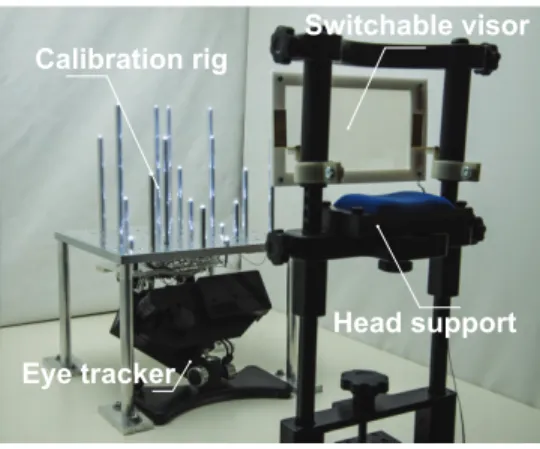
Switchable visor Calibration rig

Eye tracker

Head support

Fig. 2. Calibration setup. EyeLink 1000 is used to track the eye movements and a chin-forehead rest is used for stabilization. Coordinates space of the calibration targets and shapes are aligned with sockets permanently mounted on the table. A switchable visor is used to control the on-site of stimuli. A custom-built calibration rig is used with 20 LEDs mounted as calibration targets.

question, namely if geometric features of the shape may be salient, i.e., attract attention regardless of viewing conditions.

3.1 Setup

For eye tracking, we use an EyeLink 1000 table top device, which is routinely used in a variety of eye tracking experiments. The eye tracker consists of a camera and an integrated IR illumination (as shown in Figure 2). The camera and the light source need to have free view on the eyes, with the angle to the line of sight being limited. As eye tracking has limited angular accuracy, the spatial accuracy decreases with the distance to the observer. This motivates us to bring the shape in the experiment close to the observer such that the error in relating the gaze to the shape is small, while still keeping the eye tracker in its working range with distinct corneal reflections.

We accomplish the requirements of the eye tracking device and our goal to place the shape close to the observer by placing the shapes onto a fixture that allows placing the eye tracker under it (see Figure 2). The fixture is placed with its front edge at a distance of 320 mm to the observer, allowing the presentation of objects at an average distance of about 430 mm (see Figure 1 for a schematic illustration of related distances). The fixture is made of aluminum.

The base is a block with dimensions 300 mm × 300 mm × 12 mm . It is

mounted onto four cylindrical legs with a diameter of 20 mm, which

fit into sockets permanently mounted to the table. There are two

copies of the fixture. One base plate contains a raster of 9 × 9 screw

mounts with grid constant 40 mm. The screw mounts serve to hold

the legs as well as 20 tubes with calibration targets as shown in

Figure 2. The other base plate only has the four corner mounts for

the legs and 4 holes to hold a connector for the base of the shapes as

shown in Figure 4. Machining precision for these parts is reportedly

on the order of 2 / 10 mm. This allows presenting the shapes in a

coordinate frame that is very well aligned with the coordinate frame

of the calibration targets.

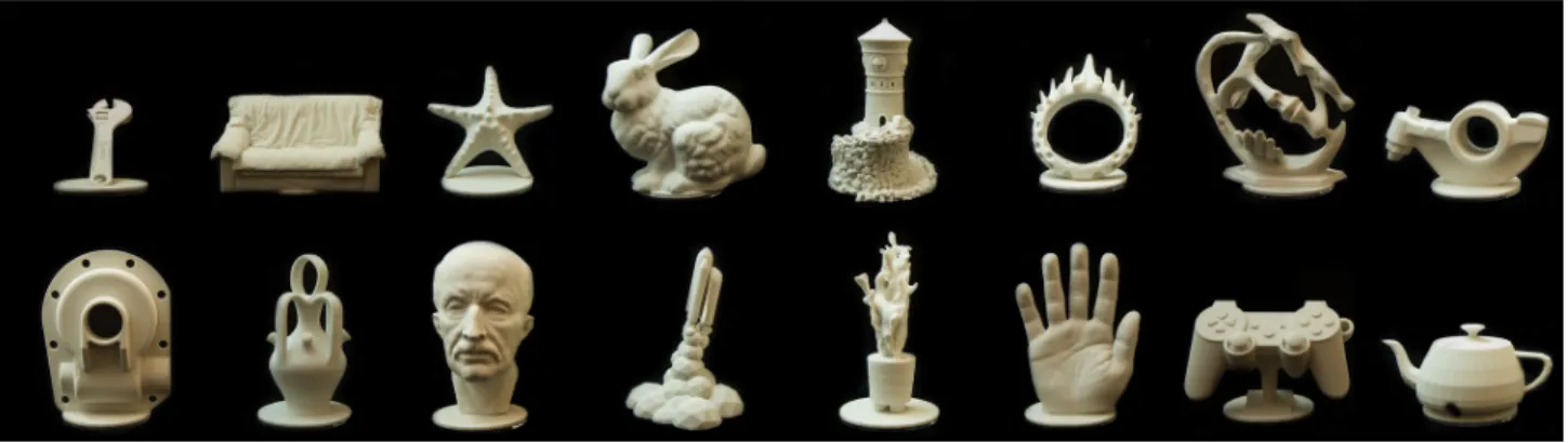
Fig. 3. The whole stimuli set of 16 shapes printed in sandstone.

Object base

Socket

Fig. 4. During viewing, 3D printed stimuli are placed in front on a fixture, which is mounted into the sockets on the table. The coordinate frame of shapes is aligned with the calibrated space by mounting the two identical fixtures in the sockets that are permanently mounted onto the table.

The calibration targets are LEDs. Each LED is mounted onto the top of an aluminum tube, wired through the tube and the screw hole. The tubes have different lengths and the LEDs cover a volume of 150 mm

³

(consistent with the size of the shapes, see below). LEDs are arranged in space as evenly as possible while not being occluded.

They are controlled by an Arduino board, so that the active time of each of the LEDs can be recorded and aligned with the data from the eye tracker. While the accuracy of the positions of the tubes on the base plate is high, the exact heights of the LEDs relative to the top of the tubes vary slightly, and the angular deviation of the screw mounts potentially translates into significant displacement at the top of the tube. To compensate for this, we measure the positions of the LEDs using a recent structure from motion tool [Schönberger and Frahm 2016]. We took 10 photographs with constant camera parameters of the calibration rig while all LEDs are illuminated. In each image, we identify the four corners of the base plate by fitting lines to the edges of the base and intersecting them. The front left corner serves as the origin of the coordinate system. We fit a quadratic function to the smoothly varying brightness of the LEDs in

the photographs. This yields the LED centers with subpixel accuracy.

The resulting reconstruction has a reported average accuracy of 0 . 6 mm in the positions of the LEDs. The reconstructed positions are consistent with the design of the fixture.

The whole setup is enclosed by a box with diffuse white walls to avoid presenting visually interesting features apart from the stimulus. The front side of the box is open, leaving space for a head and chin rest.

3.2 Selection of stimuli

It is well known that both low-level features, such as contrast and edges, and high-level features, such as faces, consistently attract visual attention [Gottlieb et al. 2013; Henderson and Hollingworth 1999; Tatler et al. 2011]. In order to best investigate how low-level features generated by the geometry of a region and high-level fea- tures embedded in the shapes contribute to the visual saliency, we try to select a set of models that represent a broad generalization.

We include shapes with both smooth surface and sharp corners.

Symmetrical shapes, including those with repetitive geometric fea- tures, are also selected, although we suspect that repetitive features could make it difficult to find a consistency among observers. Even if such features draw attention, the number of fixations on each of them could still be small. Inspired by [Lau et al. 2016], we also include man-made artifacts (e.g., teapot and spanner), which might have task-related affordances (e.g., grabbing) that attract attention.

Shapes with discernible semantic features like the BUNNY-object are also included in the set to have a generalized representation.

Based on thess principles, we selecte 16 shapes (shown in Figure 3).

The number 16 is a compromise between providing enough variation and the duration required for each experiment session.

Using direct digital manufacturing for creating the physical stim- ulus has several important advantages (cf. [Wang et al. 2017a, 2016]):

(1) Because we start from the digital version and manufacturing devices are reported to have high geometric accuracy, the geometry of the physical artifact is known.

(2) Digital modeling allows us to add geometry to the bottom of the shape, enabling a connection to the experimental setup in a controllable way.

(3) The material is homogeneous.

The only potential problems result from some manufacturing tech- niques being limited in terms of the minimal thickness of parts in the shape as well as the largest dimensions because of limited build volume. The size of the shapes results from covering a large visual angle without being uncomfortable for humans to inspect the object while not moving their head. Other experiments suggest that an acceptable visual angle is 20

^◦

, resulting in an average size of 150 mm along the largest dimension. This size is still compatible with mass-market 3D printing.

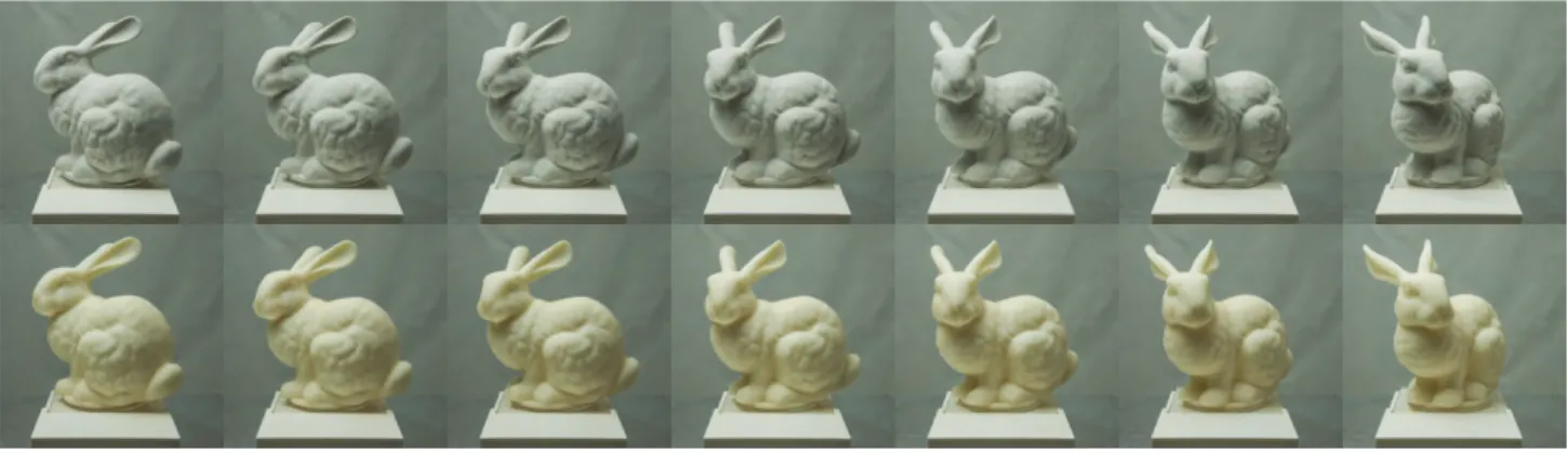
For evaluating constancy of features against change in material, we choose to manufacture each shape in two materials, using two different manufacturing devices. One set is generated using the Stratasys Uprint SE Plus fused deposition modeling device available in our lab with ABS

¹

as filament, resulting in a slightly shiny and smooth appearance. Another set is manufactured commercially using 3D ink-based printing with a diffuse material

²

. Figure 5 shows a visual comparison of the BUNNY-object printed in two materials.

To test the variation in viewing behavior, we present each shape in several orientations. For each shape we decide on an up-direction.

The different orientations result from rotating around the up-axis.

Rotation by very large angles would lead to occlusion or disocclusion of features. We feel a total range of 90

^◦

is sufficient. One may expect that for very small angles of rotation, the resulting visual stimulus in the experiment hardly changes, so this would add little information.

We split the 90

^◦

into steps of 15

^◦

(see Figure 5 for example). To facilitate an accurate presentation at different angles, we add a flat 24-gon to the base of the shape. Adding this 24-gon to the shape before manufacturing has the advantage that the angle of the vertices of the polygon relative to the geometry is well-defined.

The set of 7 orientation together with the two different materials leads to 14 different experimental conditions for each of the 16 shapes.

3.3 Presentation

We believe a lighting situation that is common for humans leads to the most meaningful results. Consequently, a single light source is placed above and slightly to the left (see illustration in Figure 4) of the shapes. This leads to different surface scattering properties of shapes printed in ABS comparing to shapes printed in sandstone.

We use a luminance meter to measure the amount of light reflected from the surface and for shapes printed in ABS it is 74 cd / m

²

and for shapes printed in sandstone it is 42 cd/m

²

. In future work, it would be interesting to include more lighting conditions by varying the number of light sources, directions and intensities. Determining a good set of conditions to study variations for human perception is an interesting question.

It is important that each visual stimulus is presented at once . The underlying idea of analyzing saliency by eye tracking is that an unknown stimulus is explored, and the first milliseconds after the stimulus became present are indicative for the most important features. This can only be achieved by blocking the observers view while setting up the shape on the fixture. We wish to avoid any moving objects in front of the observer, as moving objects tend to

1ABSplus P430XL

2We printed at Shapeways using sandstone.

draw attention. We would also like to avoid any evasive motion of the observer’s head, which would invalidate the calibration. For this reasons we mount a sheet of polymer-dispersed liquid crystal (PDLC) switchable diffuser on the chin-forehead rest and the diffuser is controlled by an Arduino circuit. In its transparent condition, PDLC switchable diffuser is reported to have 90% transmission.

In opaque state, the material exhibits approximately 80% haze (i.e.

scatters incoming visible light), making it virtually impossible for participants to see through [Lindlbauer et al. 2016]. Arduino control allows us to record the time of the onset of the stimulus and to synchronize with the recorded eye positions. Figure 6 shows the view of an observer when the BUNNY-object is presented and the occluded view is shown in the right corner. No significant change of pupil size is observed when the diffuser is switched between its two conditions.

4 DATA COLLECTION 4.1 Observers

We recruited n = 78 participants (mean age = 24, SD = 4.5, 32 fe- males) for the experiment. They had normal or corrected to normal visual acuity and no (known) color deficiencies. 8 observers failed to calibrate the eye-tracker with the required accuracy, which left us with a dataset of 70 observers viewing 16 shapes. Importantly, all participants were naive with respect to the purpose of the exper- iment. Consent was given before the experiment and participants were compensated for their time.

4.2 Eye movement recording

The experiment was conducted in a quiet room and shapes were presented on the fixture 430 mm in front of the observer. The largest visual span is 20

^◦

, resulting from 150 mm being the largest dimen- sion of all shapes. Binocular eye movements were tracked with an EyeLink 1000 in remote mode and calibration was performed with our custom-built calibration fixture.

In calibration 20 LEDs were lit up one after another in random order with the first one being repeated once at the end, resulting in 21 targets in total. Recorded eye movements for the first LED is discarded and we only use the more reliable data from the second repeat.

4.3 Task

Observers read the written task beforehand and were instructed to look at and inspect the shapes. The exact task is written as "Look at each object. See if anything is unusual or odd about the object.

At the end of the experiment we will ask you to point out any observations you made. We will show the objects again, so you do not have to memorize them.". We do so to encourage observers actively viewing each shape without introducing an additional task.

As an experimental task in eye tracking based perception studies

is often designed as a trade-off between motivating observers to

actively perceive the stimuli without introducing systematic bias

and reducing the influence of noise and fatigue, we introduced such

visual search task in the experiment. Observers might interpret the

task differently but we do not observe any bias in the collected data,

which coincides with the visual search literature as well [Godwin

Fig. 5. Experimental conditions of one stimulus. Each shape is printed in two materials and presented in 7 viewing directions. Here we see an example of the Stanford BUNNY printed in ABS shown in the first row. The second row shows the shape printed in sandstone. From left to right we see all seven viewing directions presented in the experiment.

Fig. 6. View of an observer during stimuli presentation. An occluded view when the switchable diffuser is opaque is shown in the bottom corner.

et al. 2015; Monty et al. 2017]. Most observers reported that nothing is unusual except there are several objects which they were unable to identify. All of them could describe details of the viewed shapes and report their perceived aspects.

4.4 Procedure

After reading the task, observers were introduced to the experimen- tal setup and the detailed experimental routine. 16 objects were divided in two blocks with each being viewed for 5 seconds. Each observer only views one object in one condition and viewing order is randomized for each observer. Calibration and validation were conducted before each viewing block while validation is essentially a repeated procedure of calibration. We verify the calibration ac- curacy in validation and it took approximately 6 minutes for each block on average. As each configuration of one object is viewed for 5 seconds, we can easily take any subset for analysis. Although viewing order is only randomized without guaranteeing that the space of all possible viewing orders are sampled evenly, such sim- ple randomization is more than sufficient to investigate whether viewing behavior changes over time.

One practice block was conducted at the beginning, which con- sists of calibration, validation and one shape (a horse) for viewing.

Through the practice block, observers are familiarized with the experimental procedure as well as the tasks they need to perform.

We use the velocity-based fixation detection algorithm provided by EyeLink and on average there are 15 fixations in each trail of viewing one shape. Material, viewing direction and shapes all have no significant influence on the amount of fixations.

5 MAPPING

An appealing feature of the 2D to 2D mapping approach is that it can be developed from minimal assumptions: identical pupil positions identify identical positions on the stimulus; and small displacements of stimuli induce small displacements of pupil positions. Mathemat- ically, this means the mapping can be approximated by a smooth function, and practice shows that low order polynomials are suffi- cient. In particular, while some models are derived from additional assumptions on the geometry or physiology of the problem, their success is independent of the validity of the assumptions. This is important, because in many cases such assumptions are difficult to test experimentally.

Our goal is to relate pairs of pupil positions to the attended points in space. We believe this is possible because of vergence. We wish to also base our approach on minimal assumptions. In particular we want to avoid identifying individual pupil positions with eye rays and then intersecting these rays, because in this approach calibration is usually not directly optimized for the resulting positions in 3D but rather for the directions of the rays. In the following we develop a model that allows directly optimizing for the positions of the calibration targets.

Based on the established mapping between pairs of pupil posi-

tions and calibration targets, we analyze the error and model it

as a Gaussian distribution. We can then estimate the probability

distribution of a fixation on the provided three-dimensional object,

simply as the restriction of the Gaussian distribution of the fixation

in space to the object’s surface.

5.1 Mapping function

We consider a pair of pupil positions p =

p

l

p

r

∈ R

⁴

, (3)

where the subscripts l and r refer to the left eye and the right eye, respectively. Our goal is to establish a mapping f : R

⁴

7→ R

³

that identifies pairs of pupil positions with fixated points in space directly. The parameters governing f should be estimated directly from the known positions of the calibration coordinates x

i

∈ R

³

and the corresponding pairs of pupil positions p

i

measured in the calibration phase.

We develop a parametric model for f based on geometric reason- ing. As mentioned before, as long as the mapping provides sufficient accuracy, it is irrelevant whether our geometric assumptions are valid. Still, it makes sense to provide at least the precision of an idealized situation.

First, we assume that lines of sight have a common center for each eye and denote them by e

l

, e

r

∈ R

³

. The pupil positions are mapped to affine planes in R

³

using homogenous pupil positions ( p

_l

, 1 )

^T

, ( p

r

, 1 )

^T

and transformations T

_l

, T

r

∈ R

^3×3

. Then the two half-lines emanating from the centers are defined as the lines passing through the eye centers and the pupil position mapped to the affine plane:

h

l

( λ

_l

) = e

l

+ λ

_l

T

l

p

l

, λ

_l

> 0

h

r

( λ

r

) = e

r

+ λ

r

T

r

p

r

, λ

_l

> 0 . (4) We may ask that the two affine planes for mapping the pupil posi- tions coincide, and that the recovered geometry for the eye centers and the affine planes are consistent with the desired world coordi- nate system. Because the planes coincide, for any point x in space we find

x = h

l

(λ

_l

) = h

r

(λ

r

) = ⇒ λ

_l

= λ

r

= λ, (5) and the parameter λ is a linear function of the distance of the point x to the eyes. When solving for λ we have

e

r

− e

l

+ λ ( T

r

p

r

− T

l

p

l

) , (6) and this is a rational function with constant nominator and a de- nominator that is linear in the pair of pupil positions. Plugging this expression back into the equations for the half lines to find the point in space x , which is a function that is linear in λ , leads to rational linear function in the pair of pupil positions. This means we can write the mapping as

f : R

⁴

7→ R

³

, f ( p ) = A

p 1

b p

1

, A ∈ R

^3×5

, b ∈ R

⁵

. (7)

There are 20 parameters in A and b , however, they share a common scale factor, leaving us with 19 degrees of freedom. Since each point in space provides 3 constraints, this means we need at least 7 cali- bration targets to estimate the mapping – usually we use more. To estimate the parameters with more constraints than unknowns we

consider the residuals

r

i

= x

i

− A

p

i

1

b p

i

1

. (8)

A common optimization goal is to minimize the sum of the squared lengths of the residuals. Based on our geometric motivation, how- ever, we really want the residuals to have non-uniform lengths: the error in pupil positions is measured on a plane; it is proportional to the error in space, however, by a factor that depends on the distance to the center of projection. In other words, we want the error to be proportional to the distance to the observer.

One way of solving this problem is to weigh the residuals with the inverse of the known distance of the calibration targets x

i

to the observer and then solve the resulting non-linear least squares prob- lem using an appropriate solver (e.g., Ceres Solver [Agarwal et al.]).

Another solution arises from the observation that the parameter λ is proportional to the distance from the observer. Recall that λ is a constant function divided by b ( p, 1 )

^T

. This means we introduce a weighted residual by multiplying with b ( p, 1)

^T

to get

r

_i^′

= b p

i

1

r

i

= b p

i

1

x

i

− A p

i

1

. (9)

These residuals are a pure linear function in the unknown coeffi- cients of A and b , so minimizing the squares leads to a homogeneous linear system. We compute the parameters using the singular-value decomposition (SVD) of the resulting system by taking the singular vector corresponding to the smallest singular value.

Based on validation we have found that the best results are achieved by optimizing the non-linear function, however, using the values computed with the SVD for initialization.

5.2 Selecting the fixations from calibration

During calibration, observers are asked to direct their gaze at the illuminated calibration markers. This usually leads to more than one fixation per calibration target. A common strategy among man- ufacturers of eye tracking devices is to select the fixations that lead to smallest residual in the estimated mapping function. We believe this approach is questionable, as it is based on the unfounded as- sumption that the mathematical mapping is an accurate model of the real world behavior.

We base our selection on the idea that in repeated presentation of the same calibration target, accurate fixation should likely reappear, while fixations that are slightly off-target should be independently distributed and are unlikely to be repeated. Our protocol consists of repeating the calibration procedure, with the main idea of having data to validate the estimated mapping. We use the validation cycle to compute distance between fixations for corresponding calibration targets and select the pair with the smallest euclidean distance.

Formally, let p

_i^j

, j ∈ { 0 , 1 , . . .} be the pupil positions for calibration target with index i in the calibration phase, and q

^k_i

, k ∈ { 0 , 1 , . . .}

the data from the validation phase. Then we select the pair argmin

j,k

∥ p

^j_i

− q

^k_i

∥ (10)

calibration targets. We then estimate an error for this mapping by taking the fixation data for the validation session. Again, this is based on the above selection. The mapped pupil position and the known calibration target yield a sequence of error vectors v

i

. We use this set of vectors to generate a first order model of the error for this mapping.

Our assumption is that the error should really grow linearly with the distance to the observer. Based on this idea we suggest to consider the error per unit distance (from the observer). For this we divide the error vectors by the distance of the corresponding target:

v

^′_i

= 1 z

i

©

­

­

­

­

« x

i

−

A p

i

1

b p

i

1

ª

®

®

®

®

¬

. (11)

Here, z

i

is the depth value of x

i

. Let m be the number of scaled error vectors (this number is 20 in most cases). Then compute the mean µ = m

⁻¹

Í

i

v

_i^′

and covariance matrix C = 1

m Õ

i

( v

_i^′

− µ )( v

^′_i

− µ )

^T

(12) for the mapping. The eigendecomposition of this matrix allows us to define an error ellipsoid :

C = QΛQ

^T

= QΛ

^1/2

Λ

^1/2

Q

^T

= MM

^T

(13) where the matrix M contains the semi-axes of the error ellipsoid.

Both, the mean and the error ellipsoid need to be understood as functions of the distance to the observer, since we have defined them based on first dividing by depth. Putting everything together, the mean and error ellipsoid are defined as

zµ, σzM. (14)

The depth z can be taken either from the calibration targets when we want to evaluate the quality of the estimated mapping, or from the estimated viewing point by applying the mapping to the pupil positions. With σ we can adjust the size of the ellipsoid to account for a desired confidence that the ellipse contains the observed points in the validation. It is common to assume a chi-squared distribution, so we can compute the confidence interval using the cumulative chi-squared distribution for three dimensions applied to σ

²

. We choose σ = 2, corresponding to an approximately 75% confidence interval.

3EyeLink 1000 User manual http://sr- research.jp/support/EyeLink%201000%20User%

20Manual%201.5.0.pdf

Fig. 7. Mapping accuracy. Averaged errors measured inmmtogether with the mean absolute errors in x, y, z direction are plotted on the left. X is the horizontal direction, Y the vertical direction and Z points to the depth direction. Error ellipsoids are visualized on the right in a top view of the experimental setup when bunny is used as the stimulus.

5.4 Accuracy of the mapping

We use the smallest singular vector of the system of linear equations described in Equation 9 as the initialization and further optimize the solution with Ceres solver. Applying our data to the mapping procedure reveals results that are on a par with or better than other results reported in the literature. The averaged distance between estimated positions and target points is 16 . 02 mm ( SD = 5 . 42), with the largest inaccuracy in depth. The mean absolute residuals in horizontal, vertical, and depth direction are 5 . 31 mm, 19 . 88 mm, 6 . 42 mm respectively (corresponding SDs are 3 . 41, 5 . 92, 2 . 67). The mean absolute residual per mm distance over all participants is 0 . 050 ( SD = 0 . 016). This translates to a mean absolute error of 15 . 03 mm at 300 mm distance and 25 . 05 mm at 500 mm distance (see Figure 7 for a comparison with bunny). The error ellipsoid for the 75% confidence interval has a mean semi-axes length of 0 . 106 , 0 . 027 , 0 . 037 per mm distance (corresponding SDs are 0 . 076 , 0 . 021 , 0 . 031).

Accuracy in the planes orthogonal to the dominant view direction is comparable to accuracies reported for eye tracking experiments on displays, only that the mapping we compute for 3D needs to accommodate the potential variation of this mapping along the depth axis. Our numbers are consistent with video-based eye track- ing experiments – where we would stress that numbers provided by manufacturers of eye tracking devices are usually based on the residuals from the fitting procedure and not from independently collected data. This way of reporting the data is highly dependent on the degrees of freedom in the model and fails to account for the inaccuracy of repeat fixations for the same target.

The error in depth is significantly larger. This is to be expected because of the small inter-ocular base line relative to the distance of the stimulus. It is difficult to find meaningful points of comparison, because the majority of 3D eye tracking experiments are done either using some type of 3D display (e.q. red-green glasses [Essig et al.

2006] or stereoscopic displays [Wang et al. 2014]) or they operate

on a single plane [Mansouryar et al. 2016]. This may lead to slightly

different results for relating vergence to positions in 3D because

vergence is controlled not just by binocular disparity but also other

depth cues [Wagner et al. 2009; Wismeijer et al. 2008]. Gutierrez

Mlot et al. [2016] appear to fit a series of mappings for stimuli

presented at varying depth and then report the error in depth for

each of them. This would mean, their mappings are conditioned on estimating depth around a fixed value, while the mapping we generate applies generally to all depths at once. Nonetheless our numbers are comparable.

While we believe using the error ellipsoid is the correct approach from a statistical point of view (see below) for counting the number of valid fixations. One may argue that very small and very large errors lead it unintuitive results: for an observer with a calibration that turned out to be highly accurate on the validation, the error ellipses are small. This means that the fixations of highly accurate observers are counted as being on the surface only when they are very close to the surface, which is implausible given the sources of error influencing the absolute positional accuracy of our setup.

Conversely, observers with a large deviation between calibration and validation get assigned to very large ellipses, which tend to intersect the surface almost regardless of their position in space.

Out of that perspective, one might want to also check how ellipses of constant size intersect the surface. For this, we adjust the longest semi-axis of the unit-distance ellipsoid to a fixed value in the interval [ . 01 , . 15 ] . These values translate to the longest semi-axes of 4 mm - 60 mm at the target distance of 400 mm. Keep in mind that the longest axis is usually along the depth direction and that errors on the order of 10 mm - 50 mm have to be accepted based on the accuracy of the eye tracker.

As we provide all the data to the public, we are certain the in- evitable minor problems that still remain will soon be discovered and the data adjusted accordingly.

⁴

6 ANALYSIS

We base the analysis on gaze density maps , generated from fixations on the surface of the object. For this we interpret the Gaussian error distribution of an individual fixation as a density and restrict it to the surface, and then sum over the fixations. We consider different sets of fixations to account for different assumptions. The resulting density maps are compared using Bhattacharyya distance.

We perform several analyses on a per-object basis: first, we com- pare pairs of observers to find out if the variability of per-observer gaze densities is smaller within conditions than across conditions.

Then, we analyze the dependence of gaze density maps on the con- ditions (viewing direction and material), i.e., does gaze behavior change for different viewing directions or materials? Lastly, we pro- vide a visualization of regions that are attended across conditions.

6.1 Generating gaze density maps on objects

It is common to aggregate fixations into gaze density maps. For this, each fixation is associated with a density function, and the density functions are summed up over the relevant fixations, weighted by the duration of the fixations [Borji and Itti 2015; Judd et al. 2012].

Based on the error analysis in the preceding section, we model the distribution of an individual fixation as a Gaussian in space: given the unit distance mean µ and error ellipsoid M for an observer and fixation position x with duration t computed from the eye tracking

4Data for all fixations collected in the experiment as well as a small tool based on WebGL that allows exploring the fixation data can be found on the project page http:

//cybertron.cg.tu- berlin.de/xiwang/project_saliency/3D_dataset.html.

sequence, we define the distribution as t

| M | exp

− σ

²

( x − x

²

µ )

^T

M

^T

M ( x − x

²

µ )

(15) The normalization factor t/| M | accounts for the fixation duration and volume of the ellipsoid, such that the resulting distribution integrates to a fixed constant proportional to t . Note that the volume of the ellipsoid is proportional to the determinant of M and that it exhibits the error of the mapping. Larger error, i.e., larger volume, should not result in more weight being given to a fixation.

To map this distribution over R

³

onto the surface we take the restriction : we consider the values of the distribution in space only in the positions of the surface. Since the surface is given as a mesh in our case, we sample the values in the vertices. Vertices are only con- sidered if they are within the 75% confidence interval. This interval defines an ellipsoid in space. To effectively collect the vertices in this ellipsoid we use an axis-aligned-bounding-box-tree [Gottschalk et al.

1996] and filter vertices in the axis aligned bounding box around the ellipsoid [Schneider and Eberly 2002]. The density map resulting from the fixations is stored as a vector f ∈ R

^V

, where V is the number of vertices in the mesh representing the stimulus object.

Several fixations are combined into one gaze density map on the surface simply by adding the values in the vertices, i.e., the gaze density representation results from fixations f

i

as Í

i

f

i

. The density function on the surface is modeled as piecewise constant. This means, we need a measure of area that is associated to each vertex.

We take the barycentric area measure [Meyer et al. 2002], and denote the diagonal matrix of vertex areas as A . The aggregated gaze density representation is normalized, so that the density integrates to one over the surface. Based on our model assumption, the integrated gazed density is the result of multiplying with the area matrix A and then summing up the vertex values. So the normalized gaze density map resulting from a set of fixations f

i

is

g = A ( Í

i

f

i

)

∥ A ( Í

i

f

i

) ∥

1

, (16)

where the 1-norm ∥ · ∥

1

implements the summation over vertices.

Naturally we combine fixation data of the same condition, i.e., the same view on the same stimulus made out of the same material.

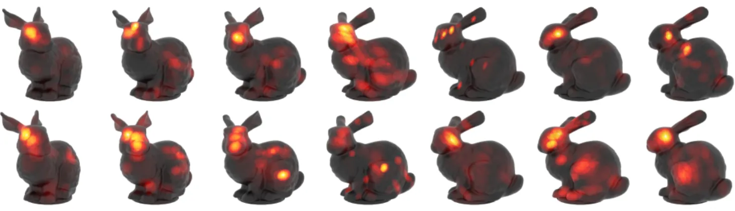
Figure 8 provides a color coded visualization of the gaze density maps for the 14 conditions of the Bunny-object used as stimulus.

For color coding we use a perceptually uniform heat map from the color maps provided by Kovesi [2015].

6.2 Measuring and visualizing the distance of gaze distributions

In order to analyze the dependence on the conditions we need a way to compare different gaze distribution functions. We suggest to use the Bhattacharyya distance [Aherne et al. 1998]. Let д, д

^′

be two continuous densities, then distance is defined as − log ∫ p

дд

^′

. This means the densities are multiplied in each point in the domain, then the square root is taken in each point, end the resulting function is integrated over the domain. For the discrete model we define the similarity vector of two (normalized) gaze density maps g, g

^′

as

s ( g, g

^′

) = q д

0

д

₀^′

, q

д

1

д

₁^′

, . . .

T

∈ R

^V

, (17)

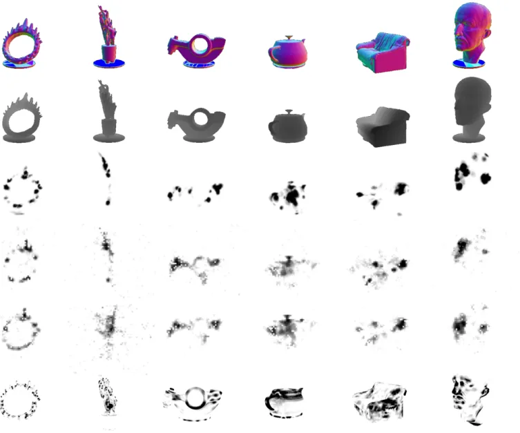
Fig. 8. Gaze density maps for the individual conditions resulting by assigning Gaussian probability density functions over the volume to each fixation and then combining them using the relative durations as probabilities. The volumetric functions are sampled on the surface and then used to assigned color values.

Columns correspond to the 7 viewing directions, upper row shows the results for ABS (slightly glossy), lower row for sandstone (diffuse).

encoding the point-wise similarity in each vertex. This representa- tion allows us to write the distance as

d ( g, g

^′

) = − log ∥ s ( g, g

^′

)∥

1

, (18) where the 1-norm ∥ · ∥

1

is a discrete version of integrating the piecewise constant function defined in the vertices over the surface.

We prefer the Bhattacharyya distance as a measure over other possible ways for comparing gaze distribution functions because it results in large distance if fixations are disjoint from each other.

What is particularly nice is that s ( g, g

^′

) in itself nicely visualizes why two functions are similar, if they are. Only regions where both gaze densities are likely to contain fixations will have non-zero values.

The concept of similarity can be extended to more than two gaze densities: Matusita [1967] introduced a measure of affinity that is based on the geometric mean of the densities (see also [Toussaint 1974]). In our context this means we extend the similarity represen- tation to a set of m gaze density maps g

⁰

, . . . , g

^m−1

as

s ( g

⁰

, . . . , g

^m−1

) =

©

­

­

­

­

­

«

д

₀⁰

· . . . · g

^m−1₀

1/m

д

1⁰

· . . . · g

^m−1 ¹

1/m

.. .

ª

®

®

®

®

®

¬

. (19)

In analogy to s ( g, g

^′

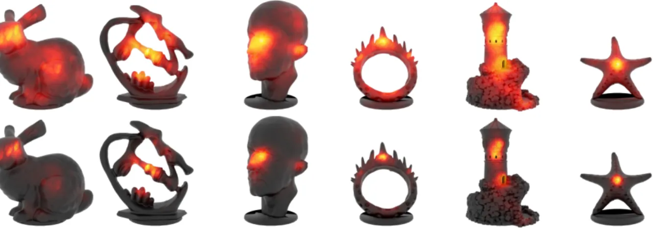
) , this extension can be used to visualize the regions that have been attended to in all gaze patterns, i.e., it high- lights stable surface features. The sum of the values in the vector representation provides a measure of similarity among the gaze distributions.

6.3 Inter-observer variation

Wang et al. [2016] have provided evidence indicating that the varia- tion across observers is smaller for the same object as stimulus than for different objects. Here we refine this question to the variation for the same object as stimulus, but different viewing conditions.

Specifically we ask: is the difference among different observers look- ing at the same object in the same condition smaller than looking at the same object in different conditions?

To do this we compute all pairwise differences of two observers on the same stimulus. There are 70 observers, resulting in

⁷⁰

2

= 2415 pairs for each object. For each object, we distinguish the 7 viewing directions and 2 materials. We consider three classes: 1) the 14 different conditions resulting from directions and materials, 2) the 7 conditions differentiating the viewing direction, but ignoring the difference in material, and 3) the 2 material conditions, ignoring the viewing direction. Figure 9 shows the resulting distributions for a subset of the stimulus objects. The distribution in blue shows all pairs, independent of condition. The three distributions in gray are pairs that are limited so that both observers are within the same class, corresponding to the classes mentioned above. Visual inspection suggests that the distributions are similar, meaning the distance between gaze density maps of two observers is not smaller for the same condition.

1 2 3

0 0 . 2 0 . 4 To test this claim statistically we apply the Kolmogorov-Smirnov test on the pairs within one of the conditions defined by the three classes vs. the distribution of all pairs. The inset to the right shows the resulting KS test statistic for the same material (1), same direction (2), and same material and direction (3). The red lines illustrate the threshold for significance at the p = 0 . 05-level. None of the within class distribu- tions differ significantly from the distribution of all pairs.

6.4 Dependence on view direction

As the inter-observer variation is high, we analyze the dependence on direction by considering all fixations for one condition, both with and without considering the difference in material. This means we are generating three different sets of gaze density maps g ( ϕ ) , g

a

( ϕ ) , g

s

( ϕ ) , where the subscripts a and s identify the materials ABS and sand- stone, and the parameter ϕ takes on discrete values for the seven viewing directions.

The following analysis applies identically to the three sets – we describe it only for the set g ( ϕ ) . We compute all

⁷

2

= 21 differences

between pairs g ( ϕ ) , g ( ψ ) , ϕ , ψ . The resulting values are illustrated

0 0 . 5 1 0 0 . 5 1 0 0 . 5 1 0 0 . 5 1 0 0 . 5 1

Fig. 9. Distributions of the distance between pairs of gaze density maps (computed as Bhattacharyya distance) per stimulus object. The blue distribution contains all possible pairs. The gray distributions are the subsets of pairs that belong to the same condition, where we distinguish between same material, same direction, and same material and direction. The distributions appear to be rather similar, suggesting that the inter-observer variation of gaze density maps is generally high.

− 0 . 5 0 0 . 5

− 0 . 5 0 0 . 5

d

,

d

,

ϕ

ψ

−0 . 5 0 0 . 5

−0 . 5 0 0 . 5

d

,

d

,

ϕ

ψ

Fig. 10. The distances between two gaze density maps for different viewing directions form a symmetric matrix. We consider the upper half of the matrix and fit a linear model to the distance. We then ask if the linear model has a significant tilt away from the diagonal, meaning that larger angular distances result in large distances between the gaze density maps. The two materials are considered separately (upper and lower illustration), as well as combined (not shown here). The distance of the gaze densities is color coded, ranging from blue for small distance to red for large distance. Note the similar trend in the data, but different variance.

in Figure 10, in the form of a triangular matrix. We are asking: is the difference of the gaze density maps dependent on the pair or, more specifically, is the distance smaller for small differences | ϕ − ψ | in viewing direction and growing for larger such differences? In order to answer this question we perform linear regression on the

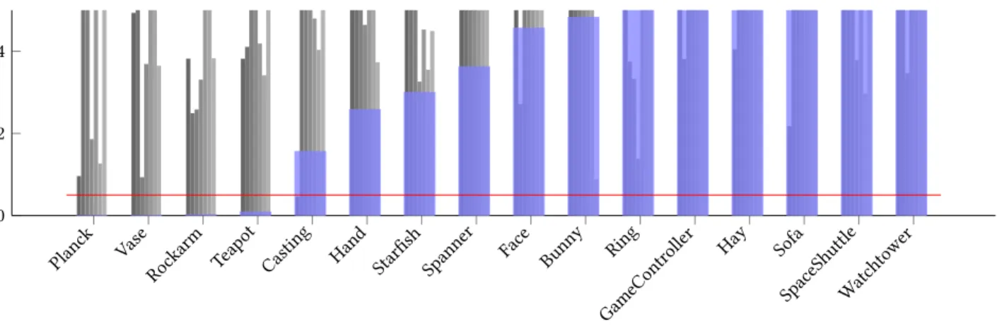
SpaceShuttle Casting W

atchto w

er

Hay SofaRing P lanck V ase

Starfish Bunny GameContr

oller Hand Face Ro

ckarm T eap ot Spanner 0

0 . 2 0 . 4

Fig. 11. The red line shows thep-value of the linear regressor exhibiting a gradient in the direction of increasing angular difference. Blue bars indicate the result for combining the fixations from the two material conditions, the lighter bars depict restrictions to one material.

data points ( ϕ,ψ , d ( g ( ϕ ) , g ( ψ )). The null hypothesis is that linear regressor is flat, i.e., that the fitted plane has normal ( 0 , 0 , 1 ) . The plane normal is found by generating the co-variance matrix of the 21 points and then taking the eigenvector corresponding to the smallest eigenvalue. The eigenvalue provides the variance σ , and the standard error is then σ/ √

n , where n = 21.

We wish to understand if the resulting normal (with standard error) is significantly different from (0 , 0 , 1). For this we need to compute how likely it is to observe a tilted normal by chance – we need a probability distribution for the plane normals. This proba- bility distribution is likely not available analytically, so we sample it: we take the same set of fixations from the 70 observers (35 in case we restrict to one of the two materials), and split it randomly into 7 groups of 10 (5) observers each. We combine the fixations and consider them as set of 7 ‘directions’ (only now they are in- dependent of the directions used in the experiment). We perform the linear regression on the distances of the 21 pairs of ‘directions’.

This process is done to generate 10,000 samples of random distance matrices similar to the ones illustrated in Figure 10, emanating from the same distribution underlying the distances among the 7 direc- tions. We find that, as expected, the mean normal of this distribution is numerically close to ( 0 , 0 , 1 ) .

Based on the sampled distribution of normals and standard errors,

we can then provide a significance level for the data generated

conservative.

Figure 11 shows the results. We find that for 11 out of 16 ob- jects there is a statistically significant dependence of distance on difference in angle at the p = 0 . 05-level. When we consider the material, fewer objects reach the significance level. Inspecting the linear regression results reveals that the planes are quite similar for the three different cases, only the smaller amount of data leads to larger standard errors for the individual materials (see, for example, the illustration for the Bunny in Figure 10 and the corresponding significance levels in Figure 11). Interestingly, some objects show a significantly flat fit, suggesting that their independence of differ- ence in viewing direction is not just coincidence and that observers attend to the same features in different views.

6.5 Material dependence

In the same way that we analyzed dependence on viewing direction, we now examine dependence on material. We ask if the difference in viewing behavior for different materials is in any way significantly different. For this test, we generate 7 different sets of gaze density maps g

⁰

( m ) , g

¹

( m ) , . . . , g

⁶

( m ) , where m takes on only two different values, and we consider all viewing directions combined or each separately. For each of the 7 sets there is only one difference that can be computed. Without considering viewing direction this is the difference of two sets stemming from 35 observers each, and in the other case it is the sets from 5 observers. As above, we are generating a random distribution for the difference values, by either considering all data of different directions and randomly splitting it into two sets of 35 observers each, or considering the data from one viewing direction and randomly splitting into 5 each. Then we can directly compute the rank of true value in the distribution of randomly generated ones to provide the significance.

Figure 12 shows the result of this test. We find that 4 models exhibit a significant difference between gaze density maps for the different materials when the viewing direction is ignored. In all other cases the dependence on material is not statistically significant.

6.6 Stable features

We wonder whether any surface features are consistently attended to by the observers across the different conditions. Based on our analysis so far, we drop the dependence on material as a condition and only consider viewing direction. This means, for each object we consider the 7 gaze density maps g ( ϕ ) consisting of the data from 10 observers each.

We may consider a region on the surface and ask whether it has been attended from 3 or more viewing directions. This can be estimated using the Matusita affinity ∥ s ( g ( ϕ ) , . . . )∥

1

for the set of

tently attended to.

Consequently, we reduce the desired range of views to either 30 or 60 degrees. This means we compute the affinity vector for sets of 3 or 5 views. For visualization purposes we combine the resulting affinity vectors. The result is depicted in Figure 14, showing that stability across 30 degrees works quite well, yet stability for 60 degrees leaves only very few regions consistently attended. From a visual inspection of the visualization we would speculate that stable features contain more semantic information, such as the eyes of the Bunny, the Face, and the windows for the watchtower, or the points of symmetry for the ring and the starfish.

7 COMPUTATIONAL MODEL OF GAZE DENSITY The idea of geometric saliency has been used in applications prob- ably because of the existence of computational models, i.e., the possibility to guess the gaze density map for a given 3D shape based on the geometry alone. Here we try to develop such a computational model based on the data we have collected and using the currently popular convolutional neural networks (CNN). This computational model can then be used in applications.

The dependence of salient features on viewing direction suggests to predict saliency based on view-dependent information unlike common geometric saliency models, which are independent of view- ing conditions [Lee et al. 2005; Song et al. 2014a].

In particular, the prediction of saliency is based on the surface normals (relative to the view coordinate system) as well as the depth information of objects. With this information as input, we train two different models for gaze density estimation.

(1) All shapes in different viewing directions are used to predict the gaze density of a shape for a new viewing direction.

(2) Shapes in different viewing directions are used to predict the gaze density of a new shape.

In the first model the computational model only needs to predict a new viewing direction, having information on the viewing behavior for the shape from other viewing directions. The second model analyzes generalization towards unknown shapes.

7.1 CNN model and training

For both models we train a simple 5-layer CNN consisting of three convolutional layers followed by a fully connected and upsampling layer. The network layout and further details are given in Figure 15.

The training input images contain the normals and depth map

of the sample objects. The first three channels of the input image

represent the surface normals at each (visible) point of the object,

the last channel represents the depth value of the underlying surface