Reflection and Refraction of Spin Waves
Dissertation
zur Erlangung des Doktorgrades der Naturwissenschaften (Dr. rer. nat.)
der Fakultät für Physik der Universität Regensburg
vorgelegt von
Johannes Stigloher
aus Rosenheim
im Jahr 2018
Promotionsgesuch eingereicht am: 8.10.2018
Die Arbeit wurde angeleitet von: Prof. Dr. Christian Back Prüfungsausschuss:
Vorsitzender: PD Dr. Andrea Donarini
1. Gutachter: Prof. Dr. Christian Back
2. Gutachter: Prof. Dr. Christian Schüller
weiterer Prüfer: Prof. Dr. Jaroslav Fabian
Contents
1 Introduction 5
I Preliminaries 7
2 Theory of Dipole-Exchange Spin Waves 9
2.1 Micromagnetism . . . 11
2.2 Magnetization Dynamics . . . 12
2.3 Magnetostatics . . . 14
2.4 Static Field and Coordinate Systems . . . 16
2.5 Dynamic Field . . . 18
2.6 Full Film Dispersion Relations in Thin Film Approximation . . . 21
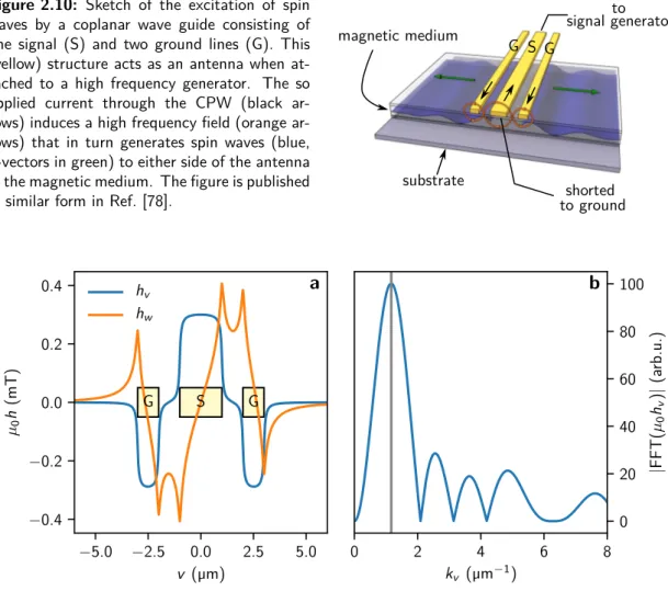
2.7 Excitation of Propagating Spin Waves . . . 26
3 Methods 31
3.1 Full Micromagnetic Simulations . . . 31
3.2 Dynamic Matrix Method . . . 32
3.2.1 Full Film . . . 33
3.2.2 In-plane Magnetized Stripe . . . 37
3.3 Time Resolved Scanning Kerr Microscopy . . . 41
3.3.1 Magneto-Optical Kerr Effect . . . 42
3.3.2 Scanning Microscope . . . 43
3.3.3 Synchronization and Modulation . . . 44
4 Propagation Characteristics 49
4.1 Applicability of the Thin Film Approximation and Surface Character of Spin Waves . . . 49
4.2 Plane Waves and Caustics . . . 52
II Experimental Results 57
5 Sample Design, Coordinate System, and Field Direction 59 6 Snell’s Law for Spin Waves 636.1 Quantitative Assessment of Wave and Sample Characteristics . . . 64
6.2 Analytical Formulation . . . 65
6.3 Bending of Spin Waves . . . 68
6.4 Angular Dependence of Snell’s Law for Spin Waves . . . 71
Contents
7 Thickness Dependence of Refraction 75
7.1 Fitting and Characterization . . . 75
7.2 Main Results . . . 77
8 Goos-Hänchen-Like Phase Shift for Spin Waves 83
8.1 Stationary Phase Method . . . 84
8.2 Field Dependence of Reflection . . . 85
8.3 Numerical Evaluations . . . 88
8.4 Angular Dependence of Reflection . . . 92
9 Summary 95
Appendix 97
A Discretization of Boundary Conditions 99 B Implementation of the Dynamic Matrix Method 101B.1 Full Film . . . 101
B.2 Stripe . . . 103
C Undersampling 105
Bibliography 107
List of Publications 119
Acknowledgment 121
1 Introduction
Spin waves are the collective excitations of magnetically ordered systems. Their respec- tive quasi particle — the magnon — is name-giving for a rapidly evolving research area called magnonics. The field aims to exploit spin waves to carry, process, and store infor- mation [1]. Potentially small wavelengths in the nanometer range [2], high frequencies in the terahertz regime [3], and Joule-heat-free transport [4] are promising features for such applications. Underlining the growing interest in magnonics and related subjects, a whole bouquet of review articles has been published in the last decade [5, 6, 7, 8, 9].
Accompanying the technological motivation, spin waves have been the subject of fun- damental research giving valuable insights in Bose-Einstein condensation [10], spin wave tunneling [11], and artificial [9] or natural magnonic crystals [12, 13]. General wave prop- erties shared with e.g. light waves or sound waves led to the study of spin wave analogs to diffraction [14, 15], interference [16, 17, 18], or the Doppler effect [19, 20]. In partic- ular, the anisotropic nature of spin wave propagation [21] — even in isotropic magnetic media — and its comparatively easy manipulation by external magnetic fields or electrical currents [22] allows for rich physics to be discovered and exploited.
To this end, this thesis focuses on the experimental investigation of spin wave reflection and refraction in the magnetostatic regime. In particular, the transmission of plane waves through an interface of two Ni
80Fe
20(permalloy, Py) films of different thickness is studied by means of time resolved scanning Kerr microscopy (TRMOKE). This optical technique allows to directly image wave fronts of incident, reflected, and refracted waves thus provid- ing information on their wavelength, angular dependence, and attenuation. Their relation is explained by incorporating the anisotropic dispersion relation, which enables us to for- mulate Snell’s law for spin waves [23]. Especially the use of a thickness step from a thick to a thin film as an interface for the refraction process provides an efficient way of spin wave steering and wavelength reduction [24] — two problems that are actively investigated in magnonics [25, 26, 27, 28, 29].
With the same technique, the reflection of plane spin waves at the edge of a Py film is examined. We observe that the phase of the reflected wave exhibits a shift with respect to the incident wave that depends on the wave vector component along the interface. Such a phase shift for a plane wave is known to lead to a spatial shift for a beam [30]. These are called Goos-Hänchen (GH) shifts and were experimentally first observed in optics [31].
Recently, they have been proposed for spin waves in different wave vector regimes and
geometries [32, 33, 34, 35]. Since our experimental results are not covered by these pre-
dictions, a numerical model is developed that provides insights into the physics governing
the shift. We can show that dipolar interactions naturally cause GH-like phase shifts for
plane spin waves in our wavelength regime and consequently expect GH beam shifts for
spin waves [36].
1 Introduction
This thesis is divided into two parts. Part I starts with an introduction to the theory of spin waves in the dipole-exchange regime that covers wavelengths in the range of nanome- ter to millimeter. Chapter 2 includes their analytic description within the framework of micromagnetism, the derivation of dispersion relations, and their excitation by means of microwave antennas. In Chapter 3, the methods utilized in this thesis are reviewed. In particular, numerical methods to obtain the spin wave spectrum in a full film (Sec. 3.2.1) and a stripe (Sec. 3.2.2) are described. Thereafter, an overview of the TRMOKE setup will be given. Part I concludes with Chapter 4, which gives insight into the unique properties of spin wave propagation by combining numerical methods, analytic dispersion relations, and first experimental results. In particular, the surface character of spin waves and spin wave caustics are discussed. The analytic dispersion relation is verified with the help of the numerical model.
Part II is dedicated to reflection and refraction experiments. Since all of these are con-
ducted on similar samples, Chapter 5 introduces their general design and the coordinate
system used. In Chapter 6, we describe our experimental results on Snell’s law for spin
waves. This includes a characterization of samples with the help of the analytic dispersion
relation, a discussion on the phenomenon of spin wave bending, as well as the comparison
to Snell’s law in optics. Chapter 7 summarizes the dependence of the refraction process on
the thickness. Finally, Chapter 8, deals with the experiments on the GH-like phase shift of
spin waves. After a review of the connection to beams, the experimental results are com-
pared to numerical simulations to reveal the connection of the GH shift to magnetostatic
interactions.
Part I
Preliminaries
2 Theory of Dipole-Exchange Spin Waves
Spin waves can be understood as a propagating phase of neighboring, precessing magnetic moments with defined wave vector
k. They are closely related to ferromagnetic resonance (FMR) [37, 38], the resonant absorption of electromagnetic energy by a ferromagnet. FMR constitutes the special case of uniform precession, i.e. a wave vector magnitude
k= 0. Spin waves with
k= 0 and
k6= 0 are sketched in Fig. 2.1. Depending on the magnitudek, the propagation is governed by either magnetic dipolar (
k <10 µm
−1) or exchange interactions (k > 100 µm
−1). The intermediate regime is called dipole-exchange spectrum, where both contributions need to be considered.
Spin waves were first described by Bloch [39] in 1930 within a microscopic theory that explained the temperature dependence of the saturation magnetization. This microscopic description is reasonable for wavelengths on the order of atomic distances and consequently describes exchange spin waves [40]. Landau and Lifshitz [41] developed a macroscopic description of ferromagnets by obtaining the equation of motion for the magnetization, a continuous vector field that averages magnetic moments of individual atoms. Nowadays, this approach is called micromagnetism [42]. It triggered the study of spin waves in the long wavelength limit: Walker [43] and others [44, 45] simultaneously solved Maxwell’s equations and Landau and Lifhsitz’s equation in bounded ferromagnets. The solutions were called magnetostatic modes or dipolar spin waves.
These classical magnetostatic modes are name-giving for the main geometries in which spin waves are typically classified. Usually, one considers a propagating spin wave with wave vector
kin the plane of a ferromagnetic film. Depending on the direction of magneti-
Figure 2.1: Sketch of a snapshot in time of two spin waves with k = 0 and k 6= 0 in a and b, respectively. Blue denotes either the spin or the magnetization, precessing around its equilibrium. The green arrows in b depict one component of the precession amplitude, which changes harmonically in space, as indicated by the sine-like green curve connecting the arrows.
2 Theory of Dipole-Exchange Spin Waves
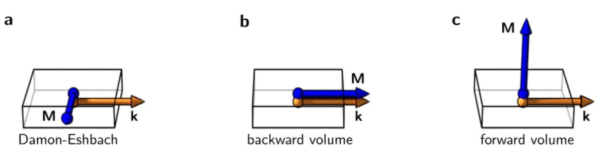
Figure 2.2: Main geometries of in-plane propagating spin waves. a Damon-Eshbach, b backward volume, andcforward volume modes.
zation
M, the modes are either called Damon-Eshbach (DE) or surface spin waves (
M⊥k,
Min the plane), backward volume (BV) spin waves (
Mkk,
Min the plane), and forward volume (FV) spin waves (
Mperpendicular to the plane), see Fig. 2.2. All three modes have unique dispersion relations, which smoothly merge into one another for arbitrary directions of
Mand
k. Especially the spin wave manifold for both the magnetization as well as the wave vector in the sample plane will be investigated in this thesis.
In addition to an in-plane propagating wave vector, all modes can exhibit a standing wave pattern across the thickness of the ferromagnetic film due to confinement in this direction. These modes are called perpendicular standing spin waves (PSSW). In general, they are not purely harmonic, i.e. they do not exhibit a defined wave vector, and crucially depend on the imposed boundary conditions at the top and bottom of the film. The simultaneous treatment of both exchange boundary conditions [46, 47] as well as electro- magnetic boundary conditions led to the development of the so called Green’s function formalism [21, 48, 49, 50]. It is applicable for the full dipole-exchange spin wave spectrum and contains both dipolar as well as exchange spin waves as limits. Following this ap- proach and Ref. [51], in the subsequent theoretical sections, the dispersion relation for all main modes are derived analytically for the lowest energy PSSW. Higher energy PSSWs are numerically investigated in Sec. 3.2.1.
Experimentally, this thesis discusses magnetostatic modes (with
Min the plane), which are more easily accessible than exchange spin waves. Wavelengths are large enough (mi- crometer – millimeter) to be spatially resolved by magneto-optical imaging techniques such as TRMOKE [52] and Brillouin light scattering (BLS) [53, 54]. Together with the all-electrical propagating spin wave spectroscopy (PSWS) [55], they comprise the main measurement techniques for this wave vector regime.
This chapter starts by shortly formulating a theoretical basis within the framework of
micromagnetism following Refs. [42, 56, 57, 58]. As already done in this introduction,
we will denote vectors with bold symbols and their magnitudes with the respective italic
symbol. In addition, tensors are also denoted with bold symbols. Unit vectors are denoted
with
ei, where the subscript
igives their direction.
2.1 Micromagnetism
2.1 Micromagnetism
The basis of micromagnetism is the description of the magnetization
M(r,t), which isa smooth, continuous vector field, defined on length scales well above the atomic scale, where the discrete nature of atoms can be neglected. This is true in both space
rand time
t[42, 58]. It can be defined as the sum of individual magnetic moments
µper volume
VM
(
r,
t) =
PV µ V
.
The vector field exists up to a material dependent Curie temperature
TC. This continuum approach enables a classical treatment of ferromagnetism, although magnetism must be regarded as a quantum mechanical phenomenon. The existence of magnetic moments
µis closely connected to the spin. The long range ordering of individual
µin ferromagnets
— which allows us to define
M(
r,
t) — has its roots in the exchange interaction. Both are fundamentally of quantum mechanical nature, but their macroscopic influence can be grasped within the theory of micromagnetism.
At temperatures below
TCthe magnetization vector is assumed to have a defined length
MSeverywhere in space. This material parameter is called the saturation magnetization.
The ground state of
Mis found by accounting for relevant magnetic field contributions
Heff. These are usually derived from the free energy density
Fvia [57]
Heff
=
−1
µ0δF
δM
, (2.1)
with
µ0= 4
π×10
−7VsA
−1m
−1the permeability of vacuum. Then, the so called Brown’s equation [42]
M×Heff
= 0 (2.2)
defines the equilibrium position of
M— aligned parallel to
Heff. In this work, three energy density contributions are considered for the derivation of
Heff[58]:
• The Zeeman energy density
Fzee
=
−µ0M·Hext, (2.3)
which describes the action of an external field
Hexton the magnetization. It is obviously favorable if the magnetization is aligned parallel to
Hext.
• The exchange energy density
Fexc=
AMS2
(
∇·Mx)
2+ (
∇·My)
2+ (
∇·Mz)
2, (2.4)
which tends to uniformly align the magnetization. Here,
Ais called the exchange
stiffness constant.
2 Theory of Dipole-Exchange Spin Waves
• The demagnetizing energy density
Fdem=
−1
2
µ0M·Hdem, (2.5)
which stems from long-ranged magnetic dipole interactions and depends on the given sample geometry. The demagnetizing field
Hdemdescribes this interaction and is the dominant contribution for spin waves discussed experimentally in this thesis.
The last two energy contributions that lead to non-local fields also define a characteristic exchange length [57]
lexc
=
s
2A
µ0MS2
(2.6)
that defines a scale, where exchange is dominant and the magnetization can thus be assumed as uniform. The sum of all contributions
F=
Fdem+
Fzee+
Fexcdefines the effective field via Eq. (2.1). It is given by
Heff=
Hext+
Hdem+
Hexcwith
Hexc
=
l2exc∆
M. (2.7)
Typically, it is not trivial to calculate
Hdemfor arbitrary sample shapes. To this end, Sec. 2.3 is devoted to derive this field from magnetostatic Maxwell’s equations. Alter- natively, one could obtain
Hdemby considering the microscopic dipolar fields originating from individual
µ. Owing to these different points of view,
Hdemis interchangeably called dipolar field, stray field (outside the sample) or magnetostatic field in the literature. Fur- ther contributions, e.g. magnetocrystalline anisotropy, anisotropic exchange, or strain are not discussed here, as they only play a minor role in our experiments.
2.2 Magnetization Dynamics
In a non equilibrium situation, where
Mis not aligned parallel with
Heff, a torque acts on the magnetization resulting in a precessional motion of the magnetization around
Heff. The temporal and spatial evolution of
Mis described by the Landau-Lifshitz-Gilbert equation (LLG) [41]
∂M
∂t
=
−γµ0(
M×Heff)
| {z }
precession
+
α MS
M×∂M
∂t
| {z }
damping
, (2.8)
with
γ=
|2mgee|the gyromagnetic ratio,
ethe electron charge,
methe mass of the electron, and
gthe Landé factor. The strength of the damping term is accounted for by a dimen- sionless material parameter, the damping constant
α. This equation preserves the lengthof
Mand the trajectory of the magnetization spirals towards equilibrium if there is no external stimulus, e.g. a driving field that preserves the precession. The two torque terms
— precession and damping — are depicted in Fig. 2.3.
To solve the LLG, we will assume a harmonic time dependence with angular frequency
ω= 2πf. Thereafter, the magnetization is divided in a space and time dependent, dynamic
2.2 Magnetization Dynamics
Figure 2.3: aThe magnetization (blue) follows a precessional trajectory driven by the torque
−γµ0(M×Heff) (green arrow). bThe dissipa- tion of energy is accounted for by the torque
MαS M×∂M∂t (orange arrow). The resulting motion is a spiral towards the equilibrium po- sition (transparent blue) given by the direction ofHeff.
part
m(
r,
t) =
m0(
r)exp(i
ωt) and a static, uniform part
Meq. It is further assumed that the precession angle is small, such that the magnitudes fulfill
m Meqand
Meq=
MS. We choose a coordinate system attached to the magnetization as depicted in Fig. 2.4. In this coordinate system, the magnetization can therefore be written as
M
(
r,
t) =
mx MS mz
.
Likewise, the field is separated into a dynamic part
hand and a static part
H, such that
Heff=
Hey+ (
hxex+
hzez).
Put into Eq. (2.8) and neglecting non-linear terms of
hand
m, the result is called the linearized LLG
i
mxωi
mzω!
=
−γµ0(−
Hmz+
MShz) + i
αmzω−γµ0
(
Hmx−MShx)
−i
αmxω!
. (2.9)
For completeness, the linearized LLG excluding damping is obtained for
α= 0 and writes i
mxωi
mzω!
=
−γµ0(−
Hmz+
MShz)
−γµ0
(
Hmx−MShx)
!
. (2.10)
The latter is the main equation solved in this thesis, as it allows for the derivation of disper- sion relations of (linear) spin waves. For this reason, expressions for
Hand
hare needed.
In the following, the necessary steps towards their analytical form in certain circumstances are given. In Sec. 3.2, techniques to solve Eq. (2.10) numerically are described.
For the discussion of spin waves in the experimentally accessible
k-vector range, the
demagnetizing energy and associated fields dictate the dispersion relation. Due to their
non-local, dipolar nature, these are typically the most demanding to derive. The following
section shall therefore give a formal basis for their understanding within the framework of
magnetostatics. Afterwards,
Hand
hare derived from the important energies in Secs. 2.4
and 2.5, which finally allows to derive the full film dispersion relations.
2 Theory of Dipole-Exchange Spin Waves
Figure 2.4:Coordinate systemxyz. The (har- monic) dynamic magnetization components are mx andmz and the static, not-time-dependent magnetization Meq will always be aligned par- allel with y. It holds true that m Meq and Meq=MS.
2.3 Magnetostatics
In the absence of currents, Maxwell’s equations for ferromagnetic media in the magneto- static limit [42, 56, 59] read
∇×H
= 0 ,
∇·B
=
µ0∇·(
H+
M) = 0 . (2.11)
The first equation implies the existence of a scalar potential function
φMthat fulfills
H
=
−∇φM. (2.12)
Together with the second Maxwell equation,
∇2φM
=
∇·M=
−ρM(2.13)
defines the magnetic charge density
ρMin reminiscence on the electrostatic potential and respective electric charge density. The field defined by Eq. (2.12) is called the demagnetiz- ing field
Hdem, which originates from
ρMand therefore
M. The usual procedure to obtain
Hdemis to find solutions for
φMand then simply take the gradient of the potential. To do so, the Green’s function
Gfor the Laplace operator defined by
∇2G
(
r) =
δ(
r)
is used, where
δrefers to the Dirac delta distribution. In three dimensions, this function is known to be
G
(
r) =
−1
4
π|r|. (2.14)
It follows that the solution to Eq. (2.13) can be directly obtained as a convolution of
Gand
ρMin a finite volume
V0via
φM
(
r) =
−1 4π
Z
V0
d
3r0∇0·M(
r0)
|r−r0|
.
2.3 Magnetostatics
Here, the primed coordinate system represents the source of the potential, i.e. a finite magnetization. If
V0is large enough such that it fully contains the region where
Mis not zero, an integration by parts yields
φM
(
r) = 1 4
πZ
V0
d
3r0∇01
|r−r0|
·M
(
r0) , (2.15)
since the surface integral vanishes. Note that far away from a region with a total magnetic moment
µ=
RV0M0, the potential has the form of a dipole potential
4π rr·µ3[59], which further illustrates the terminology
dipolar field.
In the literature, an equivalent definition of the potential is often used: after the diver- gence theorem is applied,
φMis separated into a surface and a volume part. This approach then defines the magnetic surface charge density
σS=
nM, with the outward normal n.The concept of magnetic surface charges as sources of magnetic field
Hdemoften helps as an intuitive model to understand processes involving magnetostatic interactions. As the generation of
Hdemis associated with an increase in energy (cf. Eq. (2.5)), systems avoid the creation of charges. A simple example is the magnetization lying in-plane in an infinitely extended thin film in the absence of anisotropies. In this case, no surface charges are created as
nMvanishes, which constitutes the energetic minimum. Mathematically, there is no need to define a surface, as long as boundaries to non-magnetic materials are regarded as rapid, but smooth variations of
Mto zero [42, 59].
The spatial average of the demagnetizing field in a volume
Vis finally obtained from Eqs. (2.15) and (2.12) as
<Hdem >V
=
−1 4π V
Z
V
d
3r ZV0
d
3r0∇∇01
|r−r0|
·M
(
r0) . (2.16) Note that the averaging of the field is important in many practical applications, for instance if mean fields over some sample dimensions are considered. In numerical simulations, space is usually discretized in finite volumes and the above averaging is mandatory for a correct description of
Hdem. Besides, it prevents non-physical singularities which can in principle arise at sample boundaries.
The kernel of the above expression is sometimes called Green’s function tensor [51]
defined as
Γ
(
r−r0) =
−∇∇01 4
π|r−r0|. In Cartesian coordinates,
Γis a 3
×3 matrix with elements
Γ
ij=
− ∂∂ri
∂
∂r0j
1
4π
|r−r0|, (2.17)
where
i,
jare either of the three spatial coordinates. Some properties of the original Green’s function, Eq. (2.14), are inherited, e.g. by using
∇0
1
|r−r0|
=
−∇1
|r−r0|
, (2.18)
2 Theory of Dipole-Exchange Spin Waves
the trace of
Γis
tr(
Γ) =
−∇2G(
r−r0) =
−δ(
r−r0) . (2.19) Due to interchangeable derivatives,
Γhas symmetric character i.e.,
Γ
ij= Γ
ji. (2.20)
For any body with uniform magnetization (innately true for ellipsoids), the integral in Eq. (2.16) can be evaluated independently of
M[60]. This implies the existence of a geometric demagnetizing tensor
N(e.g. Refs. [61, 42]) that directly links the magnetization with its associated field via
Hdem
=
−N·M. (2.21)
The components of the demagnetizing tensor
Nijare in general positive, accounting for the name-giving property of
Hdemthat its direction is opposite to
M, hence
demagnetizingthe sample. From Eqs. (2.19) and (2.20), we obtain that [62]
tr(
N) = 1 and
Nij=
Nji,
while the first condition is only true if the field is evaluated in the same volume as the magnetization (self-demagnetizing). For arbitrary sample geometries, the demagnetizing tensor is not easily calculated [63, 64] as the magnetization is generally non-uniform. To obtain magnetization patterns in these geometries, one usually resorts to simulations which subdivide the magnetic medium in small cells where
Mcan be regarded uniform. Then, Eq. (2.21) holds and the problem is reduced to finding an appropriate demagnetizing tensor
N, which also accounts for the case where the volume of magnetization does not coincide with the volume of the field (mutual-demagnetizing). In that case, it follows tr(
N) = 0.
The concept of demagnetizing tensors can be applied to static and dynamic parts of
Hdemand is explained in the following two sections in more detail. We will denote the static demagnetizing tensor by
Nand the dynamic demagnetizing tensor by
n.
2.4 Static Field and Coordinate Systems
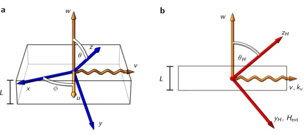
For the following derivations, we introduce a new Cartesian coordinate system with co- ordinates
u, v, and w, attached to the laboratory frame. We define two transformationmatrices
Ru
=
1 0 0
0 cos (
θ)
−sin (
θ) 0 sin (
θ) cos (
θ)
,
Rw=
cos (φ)
−sin (φ) 0 sin (
φ) cos (
φ) 0
0 0 1
, (2.22)
which link the laboratory frame with the magnetization frame via a rotation around the
axes
wand
uwith angles
φand
θ, respectively. The two coordinate systems with the
definitions of the angles are depicted in Fig. 2.5
a. A vector
rxyzand
ruvwin
xyzand
uvw2.4 Static Field and Coordinate Systems
Figure 2.5: Definition of coordinate systems. ashows the definition of angles φand θ that connect the coordinate systemsuvw andxyz. The former is defined with respect to the sample with thickness L. The vector ev will later be chosen as spin wave propagation direction. xyz is attached to the magnetization system and, as defined in Fig. 2.4,Meq is directed alongy-direction. In b, a coordinate system yHzH is similarly defined asxyz with the external fieldHext always pointing alongyH.
coordinate systems, respectively, is therefore transformed by
rxyz=
Ru·Rw·ruvw=
R·ruvw,
ruvw=
RTw·RTu ·rxyz=
RT·rxyz. The superscript T denotes a transposed matrix.
As pointed out in Section 2.1, three energy densities contribute to
Heffand have to be considered for both static and dynamic fields. In the following, we will restrict the discussion to the case where the static part of magnetization and field are considered uniform in space. Then, the exchange interaction does not influence
Has the gradient of
Mvanishes. It remains to discuss the fields associated with the demagnetizing and Zeeman energies.
For thin films, the demagnetizing tensor is particularly simple, since only the demagne- tizing tensor component
Nww= 1 is different from zero [56, 65]. Then, the demagnetizing energy density takes the form
Fdem=
µ20Mw2such that the whole static energy is given by
F
=
µ02
Mw2 −µ0HextM.
As mentioned before, a finite component
Mwwould lead to an increase in energy. There-
fore, without additional energy contributions, the magnetization will always be in-plane
for thin films. If an external field is applied in the film plane, the magnetization will be
aligned parallel to this field and the internal field strength verifies
H=
Hext. By contrast,
for an out-of-plane biased film, the effective field strength
Hhas to be deduced from the
2 Theory of Dipole-Exchange Spin Waves
energy. In
xyz,
Freads
F=
µ02 (−
Mysin (
θ) +
Mzcos (
θ))
2−µ0HextM, with the external field
Hextin the
uvwframe as
Huvwext
=
0
Hextcos (
θH)
−Hext
sin (θ
H)
.
The angle
θHis the analogon to
θwith respect to a coordinate system
yHzHdefined as shown in Fig. 2.5
b. There,Hextis pointing in
yH-direction. Equation (2.1) yields for the effective static field
Hxyz
=
−1
µ0∇MF
=
Hext,x
Hext,y
+ (−
Mysin (
θ) +
Mzcos (
θ)) sin (
θ)
Hext,z−(−
Mysin (
θ) +
Mzcos (
θ)) cos (
θ)
. (2.23)
To be compatible with this equation, the external field is transformed into
xyzto read
Hxyzext
=
RTu ·Huvwext=
0
Hext
cos (
θ−θH)
Hextsin (
θ−θH)
.
By applying the premise that
Mand
Hpoint in
y-direction, i.e. formally utilizing Eq. (2.2), the effective field is obtained from Eq. (2.23) as
H
=
0
H0
=
0
Hext
cos (
θ−θH)
−MSsin (
θ) sin (
θ)
Hextsin (θ
−θH) +
MSsin (θ) cos (θ)
. (2.24)
The
yand
z-components define two equations that determine the angle of magnetization
θand the magnitude of the effective field
Hfor a given direction and magnitude of the external field
θHand
Hext. In the experiments presented in this thesis, exclusively the case
θ=
θH= 0 is discussed, which simplifies the situation to
H=
Hext. Additionally, the case
θH= 90° is investigated analytically and numerically, since it represents the FV spin wave geometry and should therefore be considered for completeness. In this case,
θ= 90°
holds and
H
=
Hext−MSas long as
Hext > MS.
2.5 Dynamic Field
If the LLG is solved for its eigenmodes, one does not consider external driving fields.
Hence, exchange and demagnetizing fields are sufficient to describe the dynamic field
h.
First, we will seek the dynamic demagnetizing fields
hdem, induced by the dynamic
2.5 Dynamic Field
magnetization
m. From Eq. (2.16), we obtain
<hdem >V
= 1
VZ
V
d
3r ZV0
d
3r0Γ(
r−r0)
·m. (2.25) In order to derive the dynamic fields, it is most convenient to use the
uvwreference frame, as the demagnetizing fields depend on the sample geometry. In this frame, the components of the Green’s function tensor, Eq. (2.17), are given by
Γ
ij=
− ∂∂ri
∂
∂r0j
1
4
π|r−r0|,
i,
j∈ {u,
v,
w}. (2.26) Since the dynamic fields are induced by spin waves with a defined wave vector
k, it isadvantageous to evaluate the kernel in Fourier space. We utilize the Fourier representation of the rightmost part of the above equation [59, 51], i.e.
1
|r−r0|
= 1 2
π2Z
d
3ke
ik(r−r0) k2.
Using the residuum theorem, this expression can be integrated over the out-of-plane com- ponent
kwyielding a dependence on the 2D in-plane wave vector
kip=
kueu+
kvevand on an in-plane space vector
rip1
|r−r0|
= 1 2
πZ
d2k
e
ikip(rip−r0ip)e
−|w−w0|kipkip
.
This step is performed as we are interested in spin waves traveling in the plane. Differ- entiation in
rand
r0in Eq. (2.26) yields the different components of the Green’s function tensor in real space
Γ
ij(
r,
r0) =
−1 8
π2Z
d2kkikj
kip
e
−|w−w0|kipe
ikip(rip−r0ip),
i,
j6=w, Γ
wj(
r,
r0) =
−sign(w−w0) i
8π
2 Zd2kkj
e
−|w−w0|kipe
ikip(rip−r0ip),
j6=w, Γ
ww(
r,
r0) = 1
8π
2 Zd2kkip
e
−|w−w0|kipe
ikip(rip−r0ip)−δ(
r−r0) . (2.27) For the last component, condition Eq. (2.19) has been used. As already indicated in the definitions of the coordinate systems, Fig 2.5, without loss of generality,
evis chosen as propagation direction, i.e.
kip=
kvevand
kip=
|kv|. We therefore seek for solutions ofthe magnetization in the form of plane waves
m
(
t,
r) =
m0(
w)e
i(ωt−k0v), (2.28)
with a wave vector component
k0, that can be either positive or negative. Note that
kvdenotes a variable in Fourier space, while
k0is the wave vector component of the
propagating spin wave. Equation 2.28 implies that neither the dynamic magnetization
nor the dynamic field depend on the second in-plane dimension
u. The integration in
2 Theory of Dipole-Exchange Spin Waves
Eq. (2.25) can therefore be directly absorbed into the tensor via
Γ(
v,
w,
v0,
w0) = lim
Lu→∞
1 2
LuZ Lu
−Lu
d
u Z Lu−Lu
d
u0Γ(
r,
r0) . Without prefactors, the integration reads
L
lim
u→∞Z Lu
−Lu
du
Z Lu−Lu
du
0e
−i(u−u0)ku= lim
Lu→∞
4 sin
2(k
uLu)
ku2.
This expression can be identified as Dirac delta distribution 4πL
uδ(ku) [51]. Hence, inte- grals over
kuin Eq. (2.27) are readily obtained. Afterwards,
kucan be set to zero, as we allow only for one finite component
kv. It follows that Γ
uj= Γ
iu= 0 as they depend on
ku. The tensor becomes effectively two dimensional and as an example
Γ
vv(v,
w,v0,
w0) =
−1 2
πZ
dkv |kv|
2 e
−|w−w0| |kv|e
ikv(v−v0).
The expression on the right hand side coincides with the definition of an inverse Fourier transform of Γ
vvwith respect to the pair
kvand ˜
v=
v −v0. The respective Fourier components ˆΓ
ijread
ˆΓ
vv(
kv,
w,
w0) =
−|kv|2 e
−|kv| |w−w0|, ˆΓ
vw(k
v,
w,w0) = ˆΓ
wv(k
v,
w,w0) =
−i sign(w−w0)
kv2 e
−|kv| |w−w0|,
ˆΓ
ww(
kv,
w,
w0) =
−δ(
w−w0)
−ˆΓ
vv. (2.29) These functions were used in Ref. [21, 50] to derive the full spin wave spectrum of a ferromagnetic film
1. They can be utilized to elegantly rewrite the convolution defined in Eq. (2.25) as multiplication in
kv-space since the inner integration can be rewritten as
hdem
= FT
−1(ˆ
Γ·mˆ) . (2.30)
As we only allow for waves with wave vector
k0, it holds ˆ
m(
kv) =
m0δ(
kv−k0). Then, the inverse Fourier transform can be directly obtained and one integration is remaining in the out-of-plane direction
w<hdem >
=
Zd
wZ
d
w0Γˆ (
k0,
w,
w0)
·m0(
w0) e
i(ωt−k0v). (2.31) From the definitions of ˆΓ
ij, only the off-diagonal components exhibit dependencies on the sign of
k0and the sign of (
w−w0). These components, that effectively mix in- plane and out-of-plane components of magnetization and field are therefore responsible for non-reciprocal phenomena of spin wave propagation. In particular, this includes the surface character of spin waves in Damon-Eshbach geometry. A numerical discussion of
1According to Refs. [48, 49], the original derivation of the functions (2.29), are found in Chartorizhskii’s candidate’s thesis. He is one of the authors of Refs. [48, 49].
2.6 Full Film Dispersion Relations in Thin Film Approximation
this phenomenon is presented in Section 4.1.
Finally, the dynamic field associated with the exchange interaction can be straightfor- wardly derived from Eq. (2.7). It is given by
hexc
(w) =
lexc2∆
m=
l2exc ∂∂w2 −k02
m0
(w) e
i(ωt−k0v), (2.32) where
lexcwas defined in Eq. (2.6).
2.6 Full Film Dispersion Relations in Thin Film Approximation
In this work, we are mainly concerned with spin waves propagating in comparably thin films with thickness
Lnot too large with respect to
lexc. Then,
thinimplies a negligible dependence of the magnetization profile on the coordinate
w, since exchange locks themagnetization in this direction. An assumption of a constant magnetization across the thickness is called the thin film approximation [66]. Consequently, any contributions of PSSWs are automatically disregarded. This approach will be quantitatively justified by numerically solving for the full spin wave spectrum including PSSWs in Section 4.1.
In thin film approximation, the gradient in
wvanishes and therefore, by Eq. (2.32),
hexc=
−lexc2 k20m.
Since
mis assumed to not depend on
w, the integration in Eq. (2.31) can be performed on the Green’s functions tensor across the thickness
Lsuch that
Γ
ˆ
TF= 1
LZ L
2
−L2
d
w Z L2
−L2
d
w0Γˆ . This double integral without prefactors can be solved explicitly as
Z L
2
−L
2
d
w Z L2
−L
2
d
w0e
−|k0| |w−w0|= 2
L k0f
(|
k0L|)(2.33) with the function
fdefined by
f
(
x) = 1
−(1
−e
−x)
x
. (2.34)
Due to their antisymmetric structure, the off-diagonal elements of ˆ
ΓTFvanish in thin film approximation and finally, the tensor can be identified as the negative dynamic demagne- tizing tensor
n
=
−Γˆ
TF=
0 0 0
0
nvv0 0 0
nww
(2.35)
2 Theory of Dipole-Exchange Spin Waves
introduced in Section 2.3, with
nvv
=
f(|
k0L|) ,nww
= 1
−f(|
k0L|) .(2.36)
Here, we have switched the terminology from
Γto
n, since
nijcan be considered simple geometric factors that are directly utilized to obtain dynamic fields via
hdem
=
− nvv0 0
nww! m
.
In passing, it can be observed that they also fulfill the usual condition tr(
n) = 1, since source and destination of this field coincide. In addition, there are no components remain- ing that depend on the sign of
k0. We will therefore drop the subscript in the following, since
k=
|k0|=
|k|.Now that we have obtained all dynamic fields in linear relation to
m, we are prepared to solve the linearized LLG, Eq. (2.10), defined in the
xyzframe for its eigenmodes. All fields and in particular the demagnetizing field can be transformed into this frame by
hxyzdem
=
−R·n·RT·mxyz.
Note that in order to perform this rotation,
nneeds to be three dimensional. Demagnetiz- ing, exchange, and external fields are used in the following two subsections to derive the dispersion relations
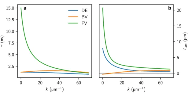
ω(k) in the main geometries. When the damped LLG, Eq. (2.9), isused, the dispersion becomes complex and the imaginary part
=(ω) =
1τcan be identified as the reciprocal of a characteristic damping time
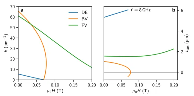
τ. Its relation to the attenuation length
Lattof a propagating spin wave is defined as [56]
Latt
=
vGτ, (2.37)
with
vG=
∂ω∂kthe group velocity. These important parameters will also be quantitatively discussed after their derivation. We distinguish between the initially mentioned main ge- ometries Damon Eshbach (DE), backward volume (BV), and forward volume (FV), which are depicted in Fig. 2.2. DE and BV modes are described by a shared dispersion relation for the in-plane geometry in the following. Even though FV modes are not discussed experimentally, we will shortly mention their main features for completeness.
In-plane Geometry
Since
θ= 0 holds,
Rwis enough to describe the in-plane spectrum with the angle
φ= 0 and
φ=
±π2corresponding to BV and DE, respectively. Then, the non-vanishing demagnetizing fields read
hxyzdem
=
hx hz!
=
− nvvsin
2(
φ)
mx nwwmz!
.
2.6 Full Film Dispersion Relations in Thin Film Approximation
Put into the linearized LLG, Eq. (2.10), and solving the corresponding system of equa- tions yields the in-plane dispersion relation for dipole exchange spin waves in thin film approximation
ω2
= (
γµ0)
2H+
MSl2exck2+
nvvMSsin
2(
φ)
H+
MSl2exck2+
nwwMS. (2.38) In case of finite damping, Eq. (2.9), the real part of
ωwill recover Eq. (2.38) while the imaginary part writes
=(ω
) = 1
τ
=
αγµ02
nwwMS
+
nvvMSsin
2(
φ) + 2
H+ 2
MSl2exck2, (2.39) when terms quadratic in
αare ignored.
General expressions for the group velocity and attenuation length can be derived from these, but can be quite cumbersome. If
|kL|1, however, exchange can be neglected and components
nijare expanded as
nvv ≈ |kL|
2 and
nww ≈1
−|kL|2 . (2.40)
Then, one can obtain expressions for group velocities of main directions to
vGDE=
γ2µ20MS2L4ω (1
− |kL|) , vGBV=
−γ2µ20MSL4ω
Hand consequently the attenuation lengths to
LDEatt=
vGDE·2
αγµ0
(2H +
MS) , (2.41)
LBVatt
=
vGBV·2
αγµ0