Hurricanes IV: Forecasts and risks

(1)

IA C E T H

Institute for Atmospheric and Climate Science

Forecasting TC’s Dyn. models Intensity models Risk Damage sources Damage preventing

Hurricanes IV: Forecasts and risks

http://www.ci.huntington-beach.ca.us/images/users/fire/Hurricane%20Katrina%20Response2.jpg Ulrike Lohmann (IACETH) Hurricanes IV: Forecasts and risks June 12, 2007 1 / 34

IA C E T H

Announcements for assignment 5

I

Arguments are important (for convincing the opposite camp)

I

We (Peter and Ulrike) will be neutral (in sense of argumentation for/against impact of climate change)

I

In the discussion the audience (without Peter and Ulrike) is the jury and will decide at the end of the panel discussion which camp had the more convincing arguments

Ulrike Lohmann (IACETH) Hurricanes IV: Forecasts and risks June 12, 2007 2 / 34

IA C E T H

stitute for Atmospheric and Climate Science

Motivation

Emanuel, 2005

(2)

IA C E T H

Some fundamentals

Definition: Areas of the globe prone to TC occurrence are referred to as “basins”, e.g. Atlantic basin (North Atlantic Ocean, Caribbean Sea, Gulf of Mexico)

I

Pike and Neumann (1987): Australian basin is the most difficult basin for TC forecasts. ∼ 3 day forecasts for the Atlantic basin are reasonable

I

Fraedrich and Leslie (1989): Predictability time scale for TC forecasting in the Australian basin is ∼ 24 h.

I

Aberson (1998): TC track forecasting in the Atlantic basin up to ∼ 5 days possible

Forecasting of TC’s on a short time scale (up to ∼ 1 day) is quite accurate (nowcasting) but for longer time intervals the accuracy of forecasts is strongly limited

IA C E T H

Forecast models

Different types of models:

I

Statistical models

I

Dynamical models

I

Intensity models

I

Storm surge models

I

Risk assessment models

In the following we focus on models which are used in the Atlantic basin (hurricane forecasting)

IA C E T H

Statistical models

Start with the location of the storm and time of the year

→ forecast is based upon the history of storms in the database with similar characteristics.

Example: CLIPER (CLImatology and PERsistence, Neumann, 1972): Multiple regression statistical model that utilizes the persistence of the current motion and climatological information.

Predicts future zonal/meridional movements of TC’s at 12-hr intervals to 72 hours. Used predictors:

I

Current/previous 12-hr position of TC’s

I

Current/previous 12-hr storm motion

I

Day of year

I

Maximum surface wind

CLIPER was hard to beat until the 1980’s. It’s now used as a benchmark for other (more detailed) models

(3)

IA C E T H

Statistical models

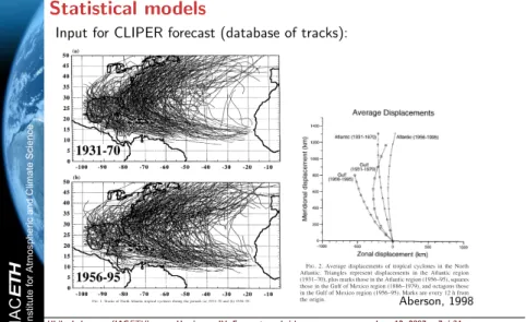
Input for CLIPER forecast (database of tracks):

DECEMBER1998 A B E R S O N 1007

FIG. 1. Tracks of North Atlantic tropical cyclones during the periods (a) 1931–70 and (b) 1956–95.

toriesiandj, xis the longitude,yis the latitude,tis time (in this case 6 h), andkis the number of 6-h time steps used. The number of pairs whose distancedij(k) remains below a threshold value,l,is counted [Nm(l)], leading to a probability estimate that the two trajectories remain within a certain distance from each other.

This value, known as the correlation integral, is given by

Cm(l)!Nm(l)/(Nm"1)², (3) whereNmis the total number of pairs of independent tracks under consideration (Grassberger and Proccacia

1008 W E A T H E R A N D F O R E C A S T I N G VOLUME13

TABLE1. Mean values of linear predictors and predictands for old and new data for the Atlantic Ocean and Gulf of Mexico basins.

Gulf of Mexico

1886–1979 1956–95

Atlantic Ocean

1931–70 1956–95

LAT—Initial latitude (!N) LON—Initial longitude (!W) INT—Initial intensity (m s^"1) DAY—Initial day number U—Initial zonal motion (m s^"1) V—Initial meridional motion (m s^"1)

20.9 89.6 28.8 249.6

"2.5 2.0

20.9 92.5 26.8 253.6

"1.6 2.5

25.5 66.1 31.3 251.2

"1.5 2.9

26.0 60.9 28.6 251.3

"2.8 1.0

FIG. 2. Average displacements of tropical cyclones in the North Atlantic. Triangles represent displacements in the Atlantic region (1931–70), plus marks those in the Atlantic region (1956–95), squares those in the Gulf of Mexico region (1886–1979), and octagons those in the Gulf of Mexico region (1956–95). Marks are every 12 h from the origin.

1984). The number of pairs of independent tropical cyclones remaining within a fixed distance of each other decreases with increasing time. The ratio ofCmtoCm#1

measures the rate at which close trajectory pairs diverge.

The order-two entropy given by K2$(1/t) exp[Cm(l) /Cm#1(l)]

forl!0 and m!% (4)

provides a lower bound for the Kolmogorov–Sinai entropy, which is itself a bound for predictability. The inverse ofK2in the region of the constant slope of correlation integral with distance defines a mean timescale over the dynamical system up to which deterministic predictability may be possible, considering ane- folding rate of the divergence of initially close trajectories.

Figure 4 shows the correlation integral for various values ofmversus the distance. The slopes of the lines do not change asmincreases, so the correlation integral is said to saturate. The region of constant slope at saturation corresponds to length scales between 50 and 500

km, a slightly larger scale than found in the Australian region. The value ofK2found in the Atlantic for suf- ficiently large values ofmcorresponds to a predictability timescale of just below 2.5 days (Fig. 5), which also is larger than that found in the Australian region. This higher value agrees with the conclusion of Pike and Neumann (1987), who found that the Australian region was the most difficult area in which to forecast tropical cyclone tracks. Because hurricane tracks are serially cor- related (Aberson and DeMaria 1994), the above calculations were again done using only those tracks that are 24 h apart from each other, with no change in the results. This gives further evidence of the stability of these calculations given the relatively small sample size.

As in any study of this type, the relatively small amount of data prevents the tropical cyclone tracks from completely covering the attractor (i.e., all possible tracks) and, thus, makes the values calculated only estimates of the true predictability timescales. Fraedrich and Leslie (1989) suggest that the predictability timescale is an upper bound to the expected ability of deterministic forecast models to predict tropical cyclone tracks, and that the limited skill of forecast models in the Australian region confirms this. However, forecast models in the Atlantic basin routinely show maximum skill at 72 h (Aberson and DeMaria 1994), slightly past the predictability timescale found in this study. The discrepancy may be due in part to the difference in the definitions of skill and error, since forecasts with very large errors may be skillful if the CLI- PER forecast errors are even larger.

4. Regression analysis and choice of predictors Two different statistical track models for the Atlantic basin have been derived for 3-day forecasts, one for the Atlantic (Neumann 1972) and one for the Gulf of Mexico (Merrill 1980). After the Merrill (1980) update to the model, the Gulf of Mexico data had not been removed from the dependent data for the Atlantic CLIPER; the two basins have been completely separated in this study. The two previous versions of CLIPER were derived by choosing from a number of predictors and their possible cross prod- ucts (Merrill 1980) and third-order polynomials (Neumann 1972) in a stepwise regression. Neumann chose the nine predictors that most impacted the explained variance of the trajectories, whereas Merrill included all of the possible predictors in the final model. Both versions chose to min-

Aberson, 1998

IA C E T H

Statistical models

Errors for CLIPER forecasts based on the old (circles) and new (triangles) model version (Aberson, 1998):

DECEMBER 1998 A B E R S O N 1013

FIG. 6. Average meridional and zonal biases of the two versions of CLIPER for all cases 1989–95. The current version of CLIPER is represented by octagons; the new version by triangles. The values shown from the origin are for 12, 24, 36, 48, 72, 84, 96, 108, and 120 h. The current version extends only to 72 h.

TABLE 5. Comparison of the absolute errors between the old and new versions of CLIPER through 120 h in km, for (a) the dependent data (1956–95) and (b) the independent data (1996).

12 h 24 h 36 h 48 h 72 h 84 h 96 h 108 h 120 h

a Old New No. of cases

111.0 108.9 1809

224.2 221.7 1699

346.5 345.2 1583

471.6 469.3 1459

718.9 706.8

1218 814.5

1102 910.7

995 1012.8

897 1110.0

805 b

Old New No. of cases

94.7 93.6 375

182.5 184.1 355

282.1 287.6 334

388.3 397.7 314

597.4 603.0 270

701.7 248

813.5 229

918.8 211

1009.3 193

1014 W E A T H E R A N D F O R E C A S T I N G VOLUME 13

FIG. 7. Average meridional and zonal biases of the two versions of CLIPER for all cases in 1996. The current version of CLIPER is represented by octagons; the new version by triangles. The values shown from the origin are for 12, 24, 36, 48, 72, 84, 96, 108, and 120 h. The current version extends only to 72 h.

ical cyclone tracks based upon satellite observations are more accurate than by any other method except reconnaissance, the updated dependent data, with tracks from the era of regular satellite and aircraft reconnaissance, are more accurate than that from which the older version of CLIPER was derived. However, the early portion of the current dependent data is before the advent of satellite observations, so CLIPER must again be derived when a 40-yr sample of satellite observations is available. Nev- ertheless, track forecast errors from the current version of CLIPER are comparable in size to those from the older version. However, large biases in track forecasts from the older version are virtually eliminated in the new, current version.

Track forecasting in the Atlantic basin has been shown to be a bit easier on average than in the Australian basin,

using techniques from nonlinear system science. Ane- folding timescale of about 2.5 days was calculated for the Atlantic basin, compared to approximately 1 day in the Australian basin. Withe-folding error growth on that scale, 5-day forecasts can be expected to show some skill. As a result, interest has increased in medium-range tropical cyclone track prediction, and the current CLIPER model provides a baseline by which the skill of such predictions can be measured.

Acknowledgments.The author would like to thank Hugh Willoughby, Pat FitzPatrick, Morris Bender, and John Kap- lan for their help in improving the manuscript, and Samuel Houston and Stanley Goldenberg in drafting the figures.

The research has been partially funded by ONR Grant N00014-94-F-0045.

1956-1995: improved data set, which is entirely within the era of regular aircraft reconnaissance.

IA C E T H

Dynamical models

Numerical weather prediction models solving the equations of motion, of thermodynamics and the continuity equation.

Two types:

I

barotropic models (move weather systems along wind fields)

I

baroclinic models (full variability and interactions)

In general baroclinic model are very computing time consuming but

usually more accurate whereas barotropic models run very fast and

it is easy to generate many forecasts with changed initial/boundary

conditions (→ ensemble forecasts)

(4)

IA C E T H

Barotropic models

Example: VICBAR (Aberson and Demaria, 1994)

Nested barotropic model that uses NCEP synoptic analyses and solves shallow–water–equations for the track prediction

Problems:

I

High vertical wind shear

I

Interacting TC pairs

IA C E T H

Baroclinic models

I

Example: Geophysical Fluid Dynamics Laboratory (GFDL) model: Limited area baroclinic model (developed for TC forecasts) on 3 nested grids:

where the inner grid follows the TC.

I

The model contains parameterizations for radiation, convection and PBL.

I

Initial/boundary conditions are taken from the Medium Range Forecast (MRF) model or National Hurricane Center (NHC) analyses.

IA C E T H

2 possibilities for initializing the vortex:

I

analysed vortex in global analysis: radius of max. wind: 350 km

I

specified vortex: radius of max. wind reduced to 60 km

Bender et al., MWR, 1993

(5)

IA C E T H

Example: Forecasting hurricane Gloria

s=specified vortex; n=vortex from NMC global analysis

IA C E T H

Comparison of hurricane track forecasts

Kurihara et al., MWR, 1993

IA C E T H

Intensity models

I

Statistical Hurricane Intensity Prediction Scheme (SHIPS, Demaria and Kaplan, 1994):

SHIPS uses standard multiple regression methods with climatology, persistence and synoptic predictors:

I

intensification potential

I

vertical wind shear

I

persistence (intensity change within the last 12 hours)

I

average 200 hPa temperature and wind components

I

average 850 hPa relative vorticity

I

day of year

I

flux average of angular momentum at 200 hPa

I

A deterministic intensity model (K. Emanuel, http : //wind .mit.edu/ emanuel /home .html )

I

Intensity forecasts with the GFDL model

(6)

IA C E T H

Intensity models (Emanuel, Nature, 1999)

IA C E T H

Lines: control simulation, +15%, -15% [Semesterarbeit Markus Fischer, 2006]

IA C E T H

Lines: control simulation, +15%, -15% [Semesterarbeit Markus Fischer, 2006]

(7)

IA C E T H

Lines: control simulation, +15%, -15% [Semesterarbeit Markus Fischer, 2006]

IA C E T H

Risk assessment models

Different damage sources:

I

precipitation (not well understood)

I

wind

I

storm surge (coupled with wind)

Several efforts to assess risks associated with TC’s winds:

1. Historic compilation of TC tracks and intensities (“best tracks”, e.g. HURDAT,

http : //www.aoml .noaa.gov/hrd/hurdat/)

2. Estimation of TC intensity along randomly produced tracks (from mathematical models using the database)

IA C E T H

Risk assessment models

Example: Combining statistical tracks with deterministic intensity models (Emanuel et al., 2006)

I

Generating (large numbers of) TC tracks using statistical methods (e.g. Markov chains, synthetic wind time series etc.)

I

Running a deterministic intensity model on these tracks

(namely the steady state model from lecture Hurricane II

including changes in the environmental state)

(8)

IA C E T H

Risk assessment models

is no less realistically represented by reanalysis data in high latitudes than in low latitudes; indeed, the flow at high latitudes may be more robust. On the other hand, the proposition that tropical cyclones move with some weighted vertical mean flow plus a correction becomes more dubious as extratropical transition occurs.

The model used to predict intensity evolution has no explicit treatment of extratropical interactions, though some of this effect in surface winds may be captured, as discussed in appendix C, by adding the translation speed to the azimuthal winds.

Cumulative frequency distributions of the maximum wind speed within 100 km of downtown Boston from both methods are compared to HURDAT and to each other in Fig. 8. The HURDAT distributions are based on only 27 events, so cau- tion should be used in interpreting the results. There are large differences in low-intensity events between the two methods, with a substan- tially larger number of weak events when using method 2. This may be owing to artificially large survival rates of weak storms in method 2, in which there are more slow-moving storms that affect Boston. The two

methods are somewhat more consistent in frequen- cies of high-intensity events, though there are still generally more in method 2.

The track of the most intense storm affecting downtown Boston in method 2, with peak winds of 84 kts, is shown in Fig. 9, together with the evolution of key quantities along the track. Much of the high wind speed in the Northeast is attributable to the rapid forward movement of the storm. As shown in Fig. 10, 93 of the 100 most intense storms affecting Boston in method 2 originate in the tropical Atlantic—6 form in the Caribbean, and 1 originates in the Gulf of Mexico and travels across peninsular Florida. Also show in Fig. 10 is the track of Hurricane Bob of 1991, the most recent storm to produce hurricane-force winds within 100 km of Boston. Its track falls well within the envelope of the 100 most intense storms of method 2.

SUMMARY. Dealing with natural hazards, from creating building codes to setting insurance premi- ums and planning for evacuations and relief efforts, depends on an accurate assessment of risk. Estimates of hurricane wind risk based directly on the historical record suffer from the overall scarcity of events, particularly in regions that experience infrequent but sometimes devastating storms. Even in regions suffering a high frequency of events, fitting standard FIG. 8. Cumulative histograms of frequency of ex-

ceedence of wind speed within 100 km of downtown Boston. Results from HURDAT data (black) are com- pared to model data for method 1 (red) and method 2 (blue). There are 27 events in the HURDAT sample versus 3,000 in methods 1 and 2.

306| MARCH 2006

probability distribution functions to observations may be inaccurate at the high-intensity end of the distribution, which is based on sparse data but accounts for a disproportionate amount of injury, loss of life, and destruction. Here we have attempted to circumvent some of these limitations by synthesizing large numbers of storm tracks and then running a deterministic hurricane intensity model along each track. This has the advantage of ensuring that the intensity of storms comforms broadly to the underlying physics, including the natural limitations imposed by potential intensity, ocean coupling, vertical wind shear, and landfall.

To synthesize hurricane tracks, we developed and tested two quite independent methods. The first con- structs each track as a Markov chain whose probability of vector displacement change depends on position, season, and the previous 6-h vector displacement, with the statistics determined by standard distribution functions fitted to observed track data. The second postulates that hurricanes move with a weighted average of upper- and lower-tropospheric flow plus a

“beta drift” correction. The flow is generated using synthetic time series of wind whose monthly mean, variance, and covariance conform to statistics derived from reanalysis data and whose kinetic energy obeys the observed ω^–3 frequency distribution characteristic of geostrophic turbulence. Shear derived from these synthetic flows is used as input to the intensity model in both track methods. The statistics of storm motion produced by both methods conform well to observed displacement statistics and to each other.

Wind exceedence probabilities for Miami, Florida, generated using both track methods agree well

with each other, with histograms based directly on HURDAT, and with estimates stemming from previously published research. Wind probabilities at Boston, Massachusetts, however, reveal the compara- tive strengths and weaknesses of the two methods.

Storms affecting high-latitude locations are almost always influenced by the interaction of tropical and extratropical systems; such an interaction is represented in the present work only by adding the storm’s translation speed to its tangential wind. Our second track method therefore cannot capture the effects of nonlinear interactions between tropical and extratropical systems, whereby either or both system may be intensified, giving a translation speed in excess of that which would have been produced by a strictly linear superposition of the preexist- ing systems. This effect is, however, represented in our first track method, because it is reflected in the displacement statistics used in the Markov chain.

On the other hand, the wind shear affecting storms generated by the first track method is independent of the storm motion. This may yield possibly large biases in tracks taken by the most severe events, as illustrated by Fig. 7. In addition, the second method may be used to generate tracks wherever the climatological reanalysis winds are deemed reliable, whereas the quality of tracks generated using the first method may be compromised in regions with little historical data. Both methods rely on an accurate estimate of the space–time distribution of storm generation.

FIG. 9. As in Fig. 6, but for the most intense of the 3,000 storms in the sample of storms affecting downtown Boston, using method 2. Dates are in August.

FIG. 10. Tracks of the 100 most intense of the 3,000 storms in the sample of storms affecting downtown Boston, using method 2. Shown for comparison (in black) is the observed track of Hurricane Bob of 1991.

307 MARCH 2006

AMERICAN METEOROLOGICAL SOCIETY |

Emanuel et al., 2006

IA C E T H

Risk assessment – normalized damages

Problem: How to estimate the damages for a long time period?

Several factors change (e.g. population and settling, costs etc.) Normalized damages taking inflation and changes in coastal

population and wealth into account

622 W E A T H E R A N D F O R E C A S T I N G VOLUME 13

TABLE 1. Damage estimates in south Florida associated with Hur- ricane Andrew. Current dollar estimates of $30 billion in damages directly related to Hurricane Andrew in south Florida. Original sources are located in Pielke (1995).

Type of loss Amount ($ billions)

Common insured private property Uninsured homes Federal disaster package Public infrastructure

16.5 0.35 6.5 state

county city schools

0.050 0.287 0.060 1.0 Agriculture

damages lost sales Environment Aircraft

1.04 0.48 2.124 0.02 Flood claims

Red Cross Defense Department Total

0.096 0.070 1.412 30.0

FIG. 1. Time series of U.S. hurricane-related losses (direct damages in millions of 1995 U.S. dollars) from 1900 to 1995 (source from Hebert et al. 1996).

makers with reliable information on which to base their expectations of future impacts.

2. Trend data

The impacts of weather on society have been defined according to a three-tiered sequence (Changnon 1996):

‘‘Direct impacts’’ are those most closely related to the event, such as property losses associated with wind damage. ‘‘Secondary impacts’’ are those related to the direct impacts. For example, an increase in medical problems or disease following a hurricane would be a secondary impact. ‘‘Tertiary impacts’’ are those that follow long after the storm has passed. A change in property tax revenues collected in the years following a storm is an example of a tertiary impact. The impacts discussed in this paper are direct impacts. Table 1 shows the direct impacts associated with Hurricane Andrew’s landfall in south Florida in 1992.

Data on the economic impacts of hurricanes are pub-

lished annually inMonthly Weather Reviewand areSEPTEMBER 1998 P I E L K E A N D L A N D S E A 625

FIG. 4. Time series of United States hurricane-related losses (direct damages in millions of 1995 U.S. dollars) from 1925 to 1995 in normalized 1995 damage amounts (utilizing inflation, coastal county population changes, and changes in wealth).

TABLE 4. Number of years with extremely high (!$1 billion,!$5 billion, and!$10 billion) normalized damage amounts for each decade. The column at the far right presents the annual average normalized damage for that particular decade.

Years!$1 billion!$5 billion!$10 billion Per year ($ billions) 1925–29

1930s 1940s 1950s

2 4 8 4

2 1 4 2

2 1 2 2

17.7 2.6 5.6 3.7 1960s

1970s 1980s 1990–95

6 5 3 4

5 2 2 1

3 1 1 1

5.2 2.7 2.2 6.6 damages to 1995 values using a simple, transparent methodology (Behn and Vaupel 1982; Patton and Saw- icki 1986). This methodology may also be useful as an independent check on the output of the more complex catastrophe models.

3. Normalized data

To normalize past impacts data to 1995 values, it is assumed that losses are proportional to three factors:

inflation, wealth, and population. The result of nor- malizing the data will be to produce the estimated impact of any storm as if it had made landfall in 1995 (cf.

Changnon et al. 1997).

Inflation is accounted for using the implicit price de- flator for gross national product, as reported in the Eco- nomic Report of the President (Office of the President 1950, 1996). Wealth is measured using an economic statistic kept by the U.S. Bureau of Economic Analysis called ‘‘fixed reproducible tangible wealth’’ and in- cludes equipment and structures owned by private busi- ness, owner-occupied housing, nonprofit institutions, durable goods owned by consumers, as well as govern- ment-owned equipment and structures (BEA 1993).

Wealth is accounted for in the normalization using a ratio (inflation adjusted) of today’s wealth to that of past years [end of year gross stock from Table A15 of BEA

Pielke and Landsea, 1998

IA C E T H

Heavy rain

In TC’s the rainfall is very strong, because of a high “precipitation efficiency”: Due to the humid environment (near saturation) the eyewall extends from the PBL to the tropopause and nearly all condensed cloud water will fall out as precipitation (nearly no evaporation of precipitation below cloud base).

Emanuel, 2005

(9)

IA C E T H

Heavy rain

Thus, the precipitation is mostly driven by the updraft motion in the eyewall which is controlled by

I

Intensification of the TC

I

Friction in the PBL

These factors control also the precipitation over land:

1. Lower intensity → less precipitation

2. Higher friction → more precipitation (remember beaker experiment: friction enhances inflow and the secondary circulation)

Usually, the first factor dominates

IA C E T H

Heavy rain

Hurricane Mitch Emanuel, 2005

IA C E T H

Tornadoes in TC’s environment

Almost all TC’s making landfall spawn at least one tornado (provided enough of the TC’s circulation moves over land) For spawning of tornadoes, the environment must have the same properties as discussed for supercell thunderstorms:

I

strong vertical wind shear

I

strong instability in low and mid levels

In the vicinity of TC’s the environment is conditionally unstable and

strong (low level) vertical wind shears occur

(10)

IA C E T H

Differences to supercell thunderstorms:

I

Instability in TC’s is merely in the lower levels (up to 3-4 km) whereas in supercell tornadoes the unstable layers extend up to 10 km

I

In TC’s the low level shear is much stronger than for

“supercell” thunderstorm environments

I

Maximum wind speed in TC’s occurs near 2-3 km, in

“supercell” thunderstorms near 10 km

⇒ In both environments the altitudes of maximum buoyancy and wind speed coincide:

IA C E T H

Tornadoes in TC’s environment

In the Northern Hemisphere the right–front quadrant of a TC is strongly favored for tornado formation (strongest vertical wind shear)

McCaul, 1991 Tornadoes in TC’s environment are usually weaker than supercell tornadoes

IA C E T H

Storm surge

The storm surge is the most damaging and deadly component of a TC: In 1970 a TC reaching Bangladesh killed over 300.000 people.

Great Cyclone of November 1970 Emanuel, 2005

(11)

IA C E T H

Storm surge

How to create a storm surge: A TC affects the elevations of the sea surface in two ways:

I

Low pressure inside the storm (∼ 1 cm/1hPa pressure deviation, see assignment 3, hydrostatic eq.)

I

Wind stress

The wind stress induces complex currents in the deep open ocean (v

c

∼ few m s

⁻¹

) but only small elevations. Problem is the interaction of wind stress with shallow water near the coast and the coast itself

IA C E T H

Storm surge

Simple experiment

3 effects:

I

Circulation of the water

I

Surface tilts to balance the friction of the wind against pressure gradient

I

Resonance: An abrupt switching off of the wind will induce a slosh back of the water. This could easily happen in nature by the moving TC and can trigger the flow in the other direction

IA C E T H

Strategies for damage prevention

Different stages for damage prevention:

I

Risk assessment

I

Long time strategies:

I

Marshlands/drying wetlands

I

No settling in high risk areas (development plans)

I

Emergency plans (including food storage and medical care) in combination with forecasts and early warning systems

I

Immediate damage prevention: dams and dikes

I

Damage prevention by better/stronger construction: roofs, doors and windows (e.g. storm shutters), walls, foundations etc.

I

Pumps

(12)

IA C E T H

Location of New Orleans

http://en.wikipedia.org/wiki/Image:Lake Pontchartrain.png http://en.wikipedia.org/wiki/Image:New Orleans Levee System.gif