energy of acoustic free oscillations will be in part transfered to the resonant modes of seis- mic free oscillations to amplify the latter amplitudes. This amplification should depend critically on how close the resonant frequen- cies are between the solid Earth and the atmosphere. The eigenfrequencies of acoustic modes are sensitive to the acoustic structure of the atmosphere (12), which varies annually (19). The above difference between0S29and other modes suggests that this annual varia- tion of the acoustic structure more precisely tunes the resonant frequencies of acoustic modes to those of seismic modes in the sum- mer of the Northern Hemisphere. We may alternatively attribute the annual variation of the oscillations to the variation of the source height, to which the excitation of coupled modes is sensitive. Thus, the observed phe- nomena are best explained by the atmospher- ic excitation hypothesis, although other pos- sibilities, such as disturbances of oceanic or- igin, cannot be ruled out.
The phenomenon of the background free oscillations represents the hum of the solid Earth, which we found to be resonant with the hum of the atmosphere through the two fre- quency windows. The excitation source of the hum may be at lowest part of the convec- tive zone of the troposphere, so that it is also responsible for the hum of the atmosphere.
The hum in the resonant windows is louder and shows a greater annual variation. The phenomenon can be understood only if the two systems of the solid Earth and atmo- sphere are viewed as a coupled system.
References and Notes
1. K. Nawaet al.,Earth Planet. Space50, 3 (1998).
2. N. Suda, K. Nawa, Y. Fukao, Science 279, 2089 (1998).
3. T. Tanimoto, J. Um, K. Nishida, N. Kobayashi,Geo- phys. Res. Lett.25, 1553 (1998).
4. N. Kobayashi and K. Nishida,Nature395, 357 (1998).
5. K. Nishida and N. Kobayashi,J. Geophys. Res.104, 28741 (1999).
6. N. Kobayashi and K. Nishida,J. Phys. Condens. Matter 10, 11557 (1998).
7. S. W. Smith,Eos67, 213 (1986).
8. G. Roult and J. P. Montagner,Ann. Geofis.37, 1054 (1994).
9. The 17 IRIS stations we analyzed were AAK (Ala Archa, Kyrgyzstan), BFO (Black Forest, Germany), COL (College Outpost, AK, USA), COR (Corvallis, OR, USA), CTAO (Charters Towers, Australia), ENH (Enshi, China), ESK (Eskdalemuir, Scotland), HIA (Hailar, Chi- na), KMI (Kunming, China), LSA (Lhasa, China), MAJO (Matsushiro, Japan), MDJ (Mudanjiang, China), PFO (Pinon Flat, CA, USA), SSE (Shanghai, China), SUR (Sutherland, Republic of South Africa), TLY (Talaya, Russia), and WMQ (Urumqi, China). The eight GEO- SCOPE stations were CAN (Mount Stromlo, Canberra, Australia), HYB (Hyderabad, India), INU (Inuyama, Japan), KIP (Kipapa, HI, USA), NOUC (Port Laguerra, Nouvelle Caledonia), SCZ (Santa Cruz, CA, USA), TAM (Tamanrasset, Algeria), and WUS (Wushi, China).
10. A. M. Dziewonski and D. L. Anderson, Phys. Earth Planet. Inter.25, 297 (1981).
11. D. C. Agnew and J. Berger,J. Geophys. Res.83, 5420 (1978).
12. S. Watada, thesis, California Institute of Technology, Pasadena, CA (1995).
13. P. Lognonne´, E. Cle´ve´de´, H. Kanamori,Geophys. J. Int.
135, 388 (1998);
14. P. Lognonne´, B. Mosser, F. A. Dahlen,Icarus110, 186 (1994).
15. H. Kanamori and J. Mori,Geophys. Res. Lett.19, 721 (1992).
16. R. Widmer and W. Zu¨rn,Geophys. Res. Lett.19, 765 (1992).
17. H. Jacobowitzet al.,J. Geophys. Res.89, 4997 (1984).
18. R. Kandelet al.,Bull. Am. Meteorol. Soc.79, 765 (1998).
19. E. L. Fleming, S. Chandra, J. J. Barnett, M. Corney,Adv.
Space Res.10, 11 (1990).
20. We are grateful to a number of people who were associated with IRIS and GEOSCOPE. We thank N.
Suda, K. Nawa, K. Nakajima, and S. Watada for com- ments on this paper.
11 November 1999; accepted 8 February 2000
Simulation of Early 20th Century Global Warming
Thomas L. Delworth* and Thomas R. Knutson
The observed global warming of the past century occurred primarily in two distinct 20-year periods, from 1925 to 1944 and from 1978 to the present.
Although the latter warming is often attributed to a human-induced increase of greenhouse gases, causes of the earlier warming are less clear because this period precedes the time of strongest increases in human-induced greenhouse gas (radiative) forcing. Results from a set of six integrations of a coupled ocean-atmosphere climate model suggest that the warming of the early 20th century could have resulted from a combination of human-induced radiative forcing and an unusually large realization of internal multidecadal variability of the coupled ocean-atmosphere system. This conclusion is dependent on the model’s climate sensitivity, internal variability, and the specification of the time-varying human-induced radiative forcing.
Confidence in the ability of climate models to make credible projections of future climate change is influenced by their ability to repro- duce the observed climate variations of the 20th century, including the global warmings in both the early and latter parts of the cen- tury (1). Several climate models accurately simulate the global warming of the late 20th century when the radiative effects of increas- ing levels of human-induced greenhouse gas- es (GHGs) and sulfate aerosols are taken into account (2– 4). However, the warming in the early part of the century has not been well simulated using these two climate forcings alone. Factors which could contribute to the early 20th century warming include increas- ing GHG concentrations, changing solar and volcanic activity (4 – 6), and internal variabil- ity of the coupled ocean-atmosphere system.
The relative importance of each of these fac- tors is not well known.
Here, we examine results from a set of five integrations of a coupled ocean-atmo- sphere model forced with estimates of the time-varying concentrations of GHGs and sulfate aerosols over the period 1865 to the present, along with a sixth (control) integra- tion with constant levels of greenhouse gases and no sulfate aerosols. In one of the five GHG-plus-sulfate integrations, the time se-
ries of global mean surface air temperature provides a remarkable match to the observed record, including the global warmings of both the early (1925–1944) and latter (1978 to the present) parts of the century. Further, the simulated spatial pattern of warming in the early 20th century is broadly similar to the observed pattern of warming. Thus, we dem- onstrate that an early 20th century warming, with a spatial and temporal structure similar to the observational record, can arise from a combination of internal variability of the cou- pled ocean-atmosphere system and human- induced radiative forcing from GHG and sul- fate aerosols. These results suggest a possible mechanism for the observed early 20th cen- tury warming.
The coupled ocean-atmosphere model that was used, developed at the GFDL, is higher in spatial resolution than an earlier version used in many previous studies of climate variability and change (7, 8), but it employs similar physics. The coupled model is global in domain and consists of general circulation models of the atmosphere (R30 resolution, corresponding to 3.75° longitude by 2.25°
latitude, with 14 vertical levels) and ocean (1.875° longitude by 2.25° latitude, with 18 vertical levels). The model atmosphere and ocean communicate through fluxes of heat, water, and momentum at the air-sea interface.
Flux adjustments are used to facilitate the simulation of a realistic mean state. A ther- modynamic sea-ice model is used over oce- anic regions, with ice movement determined by ocean currents.
Geophysical Fluid Dynamics Laboratory (GFDL)/Na- tional Oceanic and Atmospheric Administration, Princeton, NJ 08542, USA.
*To whom correspondence should be addressed. E- mail: td@gfdl.gov
The first integration is a 1000-year control case, with no year-to-year variations in exter- nal radiative forcing. After a small initial climate drift over the first 100 years, the coupled model is very stable for the remain- ing 900 years of the integration. In the other five integrations, an estimate of the observed time-varying concentrations of GHGs plus sulfate aerosols (9 –11) is used to force the model over the period 1865–2000. The radi- ative perturbations associated with sulfate aerosols are modeled as prescribed changes in the surface albedo. The latter five integra- tions are identical in experimental design, with the exception of the initial conditions, which were selected from widely separated times in the control integration after the first 100 years. These integrations have previously been used to assess regional trends in ob- served surface temperature over the latter half of the 20th century (12).
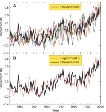
Time series of annual mean, global mean surface temperature are constructed from both observations (13) and the model integrations using surface air temperature over land and sea-surface temperature (SST) over the ocean.
The surface temperature time series from the five GHG-plus-sulfate integrations (Fig. 1A) show an increase over the last century, which is broadly consistent with the observations.
The individual runs, denoted as experiments 1 through 5, form a spread around the obser- vations, indicating the internal variability in- herent in the model.
One of the integrations (experiment 3, shown in Fig. 1B) shows a remarkable simi- larity to the observed record, including the amplitude and timing of the warming in the early 20th century. Because the model in- cludes no forcing from interdecadal varia- tions of volcanic emissions or solar irradi- ance, this suggests that the observed early 20th century warming could have resulted from a combination of human-induced in- creases of atmospheric GHGs and sulfate aerosols, along with internal variability of the ocean-atmosphere system.
Given that a combination of internal vari- ability and GHG and sulfate aerosol radiative forcing is able to produce a simulated early 20th century warming similar to that of the observed record, we can assess how likely such an occurrence is in the model. We first note that over the period 1910 –1944, the linear trend in observed temperature is 0.53 K per 35 years, whereas the trend in the five- member ensemble mean is 0.21 K per 35 years; the difference between the two is 0.32 K per 35 years. We wish to evaluate the likelihood that the trend from a single real- ization of this model (such as experiment 3) would exceed the ensemble mean by 0.32 K per 35 years (as is the case for the observa- tions). Using information from the long con- trol integration (14), we estimate that such a
difference between a single realization and an independent five-member ensemble mean oc- curs approximately 4.8% of the time, demon- strating that although the 1910 –1944 trend is a relatively rare occurrence for this model, it is still within the range of possibilities.
We now assess whether internal variabil- ity alone can account for the observed early 20th century warming, or if the radiative forcing from increasing concentrations of GHGs is also necessary. Over the period 1910 –1944 (which encompasses the warm- ing of the 1920s and 1930s), there is a linear trend of 0.53 K per 35 years in observed global mean temperature. If internal variabil- ity alone can explain this warming, compara- ble trends should exist in the control run.
Linear trends were computed over all possi- ble 35-year periods, using the last 900 years of the control run (i.e., years 101–135, 102–
136, . . ., 966 –1000). For each 35-year seg- ment, the time-varying distribution of ob- served data over the period 1910 –1944 was used to select the model locations for calcu- lating the global mean. The maximum trend in any 35-year period of the control run is 0.50 K per 35 years. This suggests that in- ternal model variability alone is unable to explain the observed early 20th century warming.
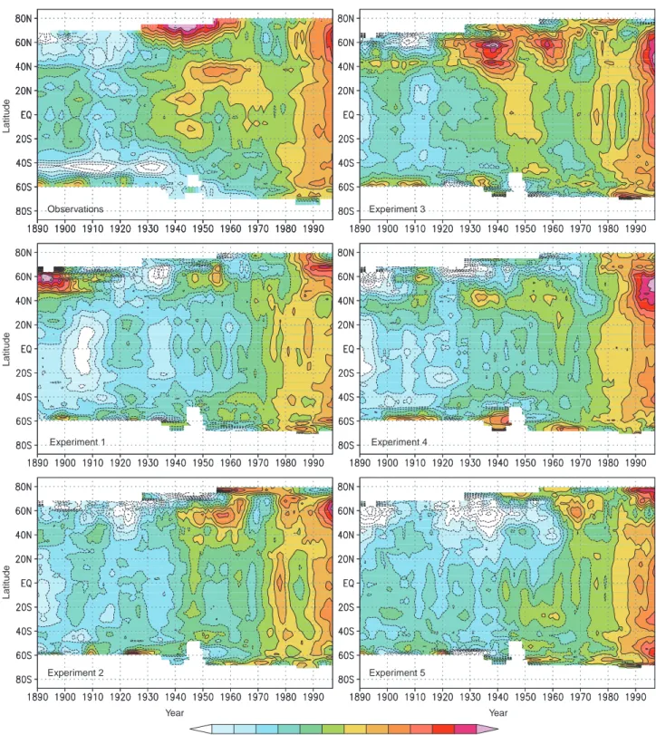
In terms of regional structure, the ob- served early 20th century warming shows a pronounced maximum at higher latitudes of the Northern Hemisphere (Fig. 2, top left). A similar warming at high latitudes of the Northern Hemisphere is also seen in experi- ment 3 (Fig. 2, top right), thereby lending credibility to the possibility that the model warming arises from physical processes sim- ilar to those important for the observed
warming. The four other GHG-plus-sulfate experiments show a range of variability in the early part of the record, illustrating the inter- nal variability of the model. Interestingly, a warming at high latitudes of the Northern Hemisphere is seen in the late 1800s of ex- periment 1, illustrating that aspects of the warming seen in the 1920s and 1930s of experiment 3 occur at other times. Also no- table is the pronounced high northern latitude cooling in the 1920s and 1930s that occurs in experiment 5. A more general warming oc- curs over the last several decades in all the experiments and in the observations, suggest- ing a robust forced response of the climate system during this period to increasing con- centrations of GHGs (2– 4).
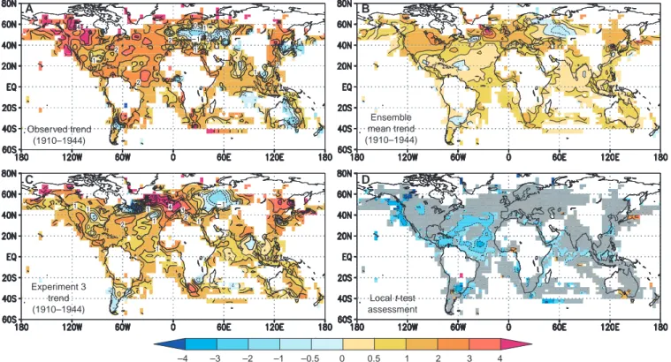
The spatial pattern associated with the early 20th century warming is further evalu- ated by computing linear trends over the pe- riod 1910 –1944 at each grid point for both the available observations and experiment 3 (Fig. 3). For the observations, the warming is largest in the Atlantic and North American regions. Although the ensemble mean trend (Fig. 3B) shows a more spatially homoge- neous pattern of warming (as expected from ensemble averaging), the pattern from exper- iment 3 (Fig. 3C) bears a considerable resem- blance to the observed trend. There are rela- tively large regional differences, however, in the northwestern North Atlantic. We can evaluate the degree to which the observed local temperature trends are consistent with the local temperature trends of the ensemble mean, taking into account the internal vari- ability of the model. Using a localttest, the gray shading in Fig. 3D denotes regions where the observed and simulated trends are consistent, whereas color shading denotes re-
Fig. 1. (A) Time series of global mean surface temper- ature from the observations (heavy black line) and the five model experiments (var- ious colored lines). Surface air temperature is used over land, while SST is used over the oceans. Units (in K) are expressed as deviations from the period 1880–1920. In con- structing the global means for the model, the model output is sampled only for times and locations where observational data are avail- able. (B) Same as (A), except that only one of the model results (experiment 3) is shown.
gions where the observed and simulated trends are significantly different at theP⫽0.10 level according to the localttest (15). By this mea- sure, the differences in the trends over the northwestern Atlantic are not statistically sig- nificant. However, the observed warming in the tropical and subtropical Atlantic is significantly underestimated by the model.
Additional characteristics of the simulated warming for which no comparable direct ob- servations are available can also be evaluated.
The ensemble mean model output was time- averaged over the period 1921–1944, and then subtracted from the 1921–1944 time- mean of experiment 3. These differences de- note the characteristics of the internal vari-
ability associated with the 1920s and 1930s warming in experiment 3. The warming was largest in the high-latitude North Atlantic, and the Nordic and Barents Seas. The upper oceans in these regions were characterized by increased temperature, salinity, and density, along with reduced sea-ice cover which ex- tended into the Arctic. The reduction in sea-
Latitude Latitude Latitude
Year Year
Observations
Experiment 1
Experiment 2
Experiment 3
Experiment 4
Experiment 5
Fig. 2. Zonal mean anomalies of surface temperature (in K) for the observations (upper left panel) and the five model experiments. Prior to plotting, all values were subjected to a 10-year low-pass filter; values are
plotted at the ending year of the 10-year period. For the model output, only times and locations for which there were observational data were used in the calculations. Anomalies are relative to the 1961–1990 climatology.
ice cover reduced near-surface albedos and appeared to play a role in increasing the radiative forcing of the surface.
The increased upper ocean density in the high latitudes of the North Atlantic is associated with an enhanced thermohaline circulation (THC) (22% larger than the ensemble mean of 14.3 Sv over the period 1921–1944; 1 Sv⫽106 m3s⫺1). The enhanced THC appears to play a role in the warming through an increased me- ridional transport of heat and an increased ocean-to-atmosphere heat flux. Additional anal- yses suggest that the enhanced THC is at least partially attributable to a persistent positive phase of the model-simulated North Atlantic Oscillation (NAO) from approximately 1910 to 1950, peaking in the late 1920s. This aspect of the simulated NAO resembles the observed NAO (16) and associated wind changes (17).
Many of the above features are seen in typical realizations of multidecadal climate variations linking the Arctic and North Atlantic in the control simulation. They also resemble previ- ously documented (18) variability in a lower resolution version of this coupled model, as well as available results from the instrumental record (19, 20) and proxy reconstructions (21) of the climate record.
Several important caveats must be consid- ered when interpreting the results of this study. First, the model has a cold bias in the
climate of the North Atlantic, leading to more sea ice than is observed in that region. Sec- ond, the simulated standard deviation of SST anomalies is larger in some parts of the North Atlantic than has been observed. The combi- nation of these factors may lead, through ice-albedo feedback, to multidecadal vari- ability which is larger than that of the real climate system, thereby influencing the inter- pretation of the above results. To shed light on this, analyses similar to those above (14) were conducted on an additional 500-year control integration, using a version of the model in which the sea-ice bias in the North Atlantic was reduced through an altered ini- tialization procedure. In⬃2.3% of the cases for that integration, the difference between a single 35-year segment and the mean of five other 35-year segments exceeded 0.32, there- by indicating a reduced likelihood (2.3%) of a single integration capturing the early 20th century warming compared with the primary model employed for this study (4.8%).
From a different perspective, a recent study (22) concluded that the high-latitude variability in a model can be rather dependent on the sea-ice model used. Unfortunately, the short- ness of the instrumental record, particularly at high latitudes, makes the evaluation of model variability on multidecadal time scales extreme- ly difficult. It is, therefore, of paramount impor-
tance to further develop and augment the instru- mental and proxy records of climate variability on decadal to centennial time scales, as well as to improve modeling capabilities.
The results of this study depend on the climate sensitivity of the model, defined as the equilibrium temperature response to a doubling of atmospheric CO2. If the climate sensitivity were smaller, then one would need either larger internal variability or additional radiative forcings to capture the early 20th century warming. The climate sensitivity of this model is approximately 3.4 K, which is in the upper half of the 1.5 to 4.5 K range cited by the Intergovernmental Panel on Cli- mate Change (23). In addition, the ensemble mean warming simulated by the GFDL mod- el over the period 1945–1995 is larger than some other coupled models (24, 25).
A recent comprehensive study (4) of the simulated climate of the 20th century sug- gested that there could be some contribution of solar forcing to the warming in the early part of the 20th century, but its quantification is problematic. Additional work (26) showed that detecting a solar influence in the early 20th century depends on which solar forcing reconstruction is used. Because the integra- tions used here do not contain interdecadal variations of volcanic or solar forcing, we can make no assessment of the potential contri-
Observed trend (1910–1944)
–4
Ensemble mean trend (1910–1944)
–3 –2 –1 –0.5 0 0.5 1 2 3 4
Experiment 3 trend (1910–1944)
Local t-test assessment
A B
C D
Fig. 3.(A) Linear trends of surface temperature (expressed as K per 100 years) over the period 1910–1944 for the available observations; (B) Same as (A) except for the five-member ensemble mean of the coupled model simulations; (C) Same as (B) but for experiment 3 only; (D) Result of a localttest comparing the ensemble mean trend and the observed trend over the period 1910–1944. Gray shading denotes regions where the ensemble mean trend is consistent with the observed trend when
one takes into account the internal variability of the coupled system as computed from the long control integration. Color shaded (nongray) regions denote an inconsistency [i.e., that the ensemble mean trend and observed trend are significantly different at theP⫽0.10 level according to a two-sided two-samplettest (15)]; this occurs for 27% of the total area for which there is sufficient observational data. The colored shading has the same units as (A).
bution of those forcings to the warming of the early 20th century. However, these results do suggest that attempts to extract the response to solar forcing by correlating estimates of solar forcing with the observed temperature record can be misleading. Although some estimates of solar forcing do correlate with the observed record, they also correlate well with our experiment 3.
If the simulated variability and model re- sponse to radiative forcing are realistic, our results demonstrate that the combination of GHG forcing, sulfate aerosols, and internal variability could have produced the early 20th century warming, although to do so would take an unusually large realization of internal variability. A more likely scenario for interpretation of the observed warming of the early 20th century might be a smaller (and therefore more likely) realization of internal variability coupled with additional external radiative forcings. Additional experiments with solar and volcanic forcing, as well as with improved estimates of the direct and indirect effects of sulfate aerosols, will help to further constrain the causes of the early 20th century warming. Our results demonstrate the funda- mental need to perform ensembles of climate simulations in order to better delineate the un- certainties of climate change simulations asso- ciated with internal variability of the coupled ocean-atmosphere system.
References and Notes
1. P. D. Jones, M. New, D. E. Parker, S. Martin, I. G. Rigor, Rev. Geophys.37, 173 (1999).
2. B. D. Santeret al.,Nature382, 39 (1996).
3. G. C. Hegerlet al.,Clim. Dyn.13, 613 (1997).
4. S. F. B. Tett, P. A. Stott, M. R. Allen, W. J. Ingram, J. F. B. Mitchell,Nature399, 569 (1999).
5. T. J. Crowley and K.-Y. Kim,Geophys. Res. Lett.26, 1901 (1999).
6. M. Free and A. Robock,J. Geophys. Res.104, 19057 (1999).
7. S. Manabe and R. J. Stouffer,J. Clim.7, 5 (1994).
8.㛬㛬㛬㛬, M. J. Spelman, K. Bryan, J. Clim.4, 785 (1991).
9. J. F. B. Mitchell, T. C. Johns, J. M. Gregory, S. F. B. Tett, Nature376, 501 (1995).
10. J. F. B. Mitchell, R. A. Davis, W. J. Ingram, C. A. Senior, J. Clim.8, 2364 (1995).
11. J. M. Haywood, R. J. Stouffer, R. T. Wetherald, S.
Manabe, V. Ramaswamy,Geophys. Res. Lett. 24, 1335 (1997).
12. T. R. Knutson, T. L. Delworth, K. W. Dixon, R. J.
Stouffer,J. Geophys. Res.104, 30981 (1999).
13. D. E. Parker, P. D. Jones, A. Bevan, C. K. Folland,J.
Geophys. Res.99, 14373 (1994).
14. For fully overlapping 35-year periods from model years 101 to 1000 (i.e., years 101–135, 102–136, . . ., 966–1000), we projected the model output onto the same grid used for the observations. The model out- put was then sampled according to the temporal and spatial distribution of observed data over the period 1910–1944 to form global mean, annual mean time series from which linear trends are calculated. This yielded a set of 866 trends of duration 35 years. We then randomly selected six samples of nonoverlap- ping 35-year periods and computed the difference between the trend in the first sample and the mean of the trends for the other five samples. This process was repeated one million times to produce a distri- bution of differences between a single trend (realiza- tion) and five-member ensemble means. Using this
distribution, we then evaluated how likely the differ- ence is between the trend corresponding to the ob- servations (viewed as a single realization) and the five-member ensemble mean trend. Differences equal to or exceeding 0.32 K/year (the difference between the observed trend and the ensemble mean model trend) occurred in 4.8% of the cases, indicating the likelihood that the observed trend is consistent with the model ensemble. This assessment depends on the assumption that internal variability in the five transient runs is similar to that in the control run.
15. The ensemble mean trend from the five GHG-plus- sulfate experiments (n⫽5) was compared with the observed trend (n⫽ 1) at each grid point (with sufficient temporal coverage), using a local two-sided two-samplettest. The population variance for thet test was estimated from 35-year trends as simulated in the 900-year control integration. For thettest, we assumed 25 degrees of freedom, based on the num- ber of nonoverlapping 35-year chunks in the control integration. Assuming only 20 degrees of freedom, the percent area rejecting the null hypothesis de- creases only slightly (from 27 to 26%).
16. J. W. Hurrell,Science269, 676 (1995).
17. J. C. Rogers,J. Clim. Appl. Meteorol.24, 1303 (1985);
C. Fu, H. F. Diaz, D. Dong, J. O. Fletcher,Int. J.
Climatol.19, 581 (1999).
18. T. L. Delworth, S. Manabe, R. J. Stouffer,Geophys. Res.
Lett.24, 257 (1997).
19. M. E. Schlesinger and N. Ramankutty,Nature367, 723 (1994).
20. M. E. Mann and J. Park,J. Clim.9, 2137 (1996).
21. 㛬㛬㛬㛬, R. S. Bradley,Nature378, 266 (1995); T. L.
Delworth and M. E. Mann,Clim. Dyn., in press.
22. D. S. Battisti, C. M. Bitz, R. E. Moritz,J. Clim.10, 1909 (1997).
23. A. Kattenberget al., inClimate Change 1995: The Science of Climate Change, J. Houghtonet al., Eds.
(Cambridge Univ. Press, Cambridge, 1996), pp. 285–
357.
24. T. P. Barnettet al.,Bull. Am. Meteorol. Soc.80, 2631 (1999).
25. M. R. Allen, P. A. Stott, J. F. B. Mitchell, R. Schnur, T. L.
Delworth,Technical Report RAL-TR-1999-084(Ruth- erford Appleton Laboratory, Chilton, Didcot, UK, 1999).
26. P. A. Stott, S. F. B. Tett, G. A. Jones, M. R. Allen, W. J.
Ingram, J. F. B. Mitchell,Clim. Dyn., in press.
27. We thank M. Allen, J. Anderson, A. Broccoli, K. Dixon, G. Hegerl, I. Held, P. Kushner, J. Mahlman, S. Manabe, and R. Stouffer for helpful contributions at various stages of the work.
6 October 1999; accepted 11 February 2000
Rapid Extinction of the Moas (Aves: Dinornithiformes):
Model, Test, and Implications
R. N. Holdaway
1* and C. Jacomb
2A Leslie matrix population model supported by carbon-14 dating of early occupation layers lacking moa remains suggests that human hunting and hab- itat destruction drove the 11 species of moa to extinction less than 100 years after Polynesian settlement of New Zealand. The rapid extinction contrasts with models that envisage several centuries of exploitation.
All 11 species of the large (20 to 250 kg) flightless birds known as moas (Aves: Dinor- nithiformes) survived until the arrival of Polynesian colonists in New Zealand (1).
Abundant remains of moas in early archaeo- logical sites show that the birds were major items of diet immediately after colonization (2–5). Indeed, the presence of moa remains was formerly used to characterize the earliest or “Archaic” period of human occupation in New Zealand [the “Moa-hunter” period (3, 6)]. Polynesian hunting and habitat destruc- tion were responsible for the extinction of all species of moa some time before European contact began in the late 18th century (1– 4, 7). Sites from the later, “Classic” Maori pe- riod lack evidence of moa exploitation. The Classic period is characterized by earthwork fortifications (the Maori term for which ispa) and occupation deposits indicating reliance on fish, shellfish, and plants for food.
Current interpretations of moa extinction implicitly or explicitly require a period of several hundred years of gradual population attrition by hunting and habitat loss: this is the orthodox model (2, 3, 5). The moa-hunt- ing period has been estimated to have lasted some 600 years, peaking 650 to 700 years before the present (yr B.P.) and ending about 400 yr B.P. (2, 3). Anderson (2) estimated the duration of moa hunting from a radiocarbon chronology of moa hunting sites and from moa population parameters based on extant ratites and African bovids. It is difficult to estimate the time of moa extinction from a series of dates on moa bones and from moa hunting sites, because confidence intervals for calibrated ages are greater than those for conventional radiocarbon ages (8), and addi- tional dates could be younger than the pres- ently perceived limit.
Reassessment of some major archaeolog- ical sites has suggested that moas were be- coming scarce by the end of the 14th century (9, 10). The earliest settlement sites date from the late 13th century (11), not the 10th or 11th century as previously thought (5). A later date for first settlement would imply that moa
1Palaecol Research, 167 Springs Road, Hornby, Christchurch 8004, New Zealand.2Canterbury Muse- um, Rolleston Avenue, Christchurch, New Zealand.
*To whom correspondence should be addressed. E- mail: piopio@netaccess.co.nz