Essays on Behavior under Risk and Uncertainty

(1)

Essays on

Behavior under Risk and Uncertainty

Inaugural-Dissertation zur Erlangung des Doktorgrades

der

Wirtschafts- und Sozialwissenschaftlichen Fakultät der

Universität zu Köln

2012

vorgelegt von Dipl.-Vw. Julia Stauf

aus Siegburg

(2)

Referent: Prof. Dr. Axel Ockenfels Korreferent: Prof. Dr. Bernd Irlenbusch

Tag der Promotion: 21. Januar 2013

(3)

i

Acknowledgements

The writing of this dissertation has been one of the greatest intellectual and personal challenges I have faced. It would not have been completed without the support, motivation and guidance of the following persons.

First and foremost, I thank my supervisor Axel Ockenfels for giving me the opportunity to work in an excellent academic environment and for guiding my research. His ideas, his knowledge and his commitment to the highest methodological standards inspired and challenged me and deepened my understanding of science.

I thank my second supervisor Bernd Irlenbusch for his valuable comments and for reviewing my thesis.

I thank my co-authors Gary Bolton, Christoph Feldhaus, Diemo Urbig and Utz Weitzel for fruitful discussions and for close collaboration in our joint research projects.

I thank my present and former colleagues Sabrina Böwe, Olivier Bos, Felix Ebeling, Christoph Feldhaus, Vitali Gretschko, Lyuba Ilieva, Jos Jansen, Sebastian Lotz, Johannes Mans, Alex Rajko, Diemo Urbig and Peter Werner for the great working atmosphere, for countless discussions of academic, general and personal matters, and for making research fun. Beyond this, I thank Vitali and Alex for repeated corrections of my beliefs about my success probability.

I thank our student helpers and in particular Markus Baumann, Andrea Fix, Gregor Schmitz and Johannes Wahlig for providing excellent research assistance.

I thank Thorsten Chmura, Sebastian Goerg and Johannes Kaiser for sharing their knowledge with me during the time I spent with them at the Bonn Laboratory for Experimental Economics, and especially for encouraging me to pursue a doctoral degree.

I thank Martin Offer for conducting an experiment on me during my diploma studies by incentivizing the hours I spent in the library. His results were highly significant both in terms of my interest in the field and my grades.

Finally, I thank my sisters Viola and Leonie Stauf, my brother Patrick Stauf, my mother Hildegard Hass-Stötzel and my father Franz-Josef Stauf for their support, patience and confidence.

(4)

ii

List of tables

Table 1: Descriptive statistics (mean, standard deviation, mode) and selected correlations ... 19

Table 2: Individual and social risk aversion depending on order ... 44

Table 3: Individual and social risk aversion with information ... 44

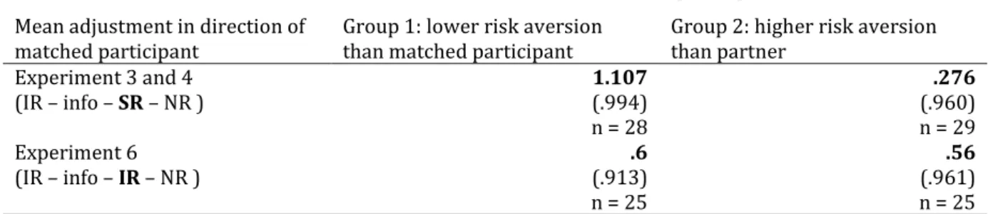
Table 4: Mean adjustment in direction of matched participant ... 45

Table 5: Adjustment of risk preferences towards the mean signal in Experiment 7 ... 46

Table 6: Payoff table treatment T1 ... 63

Table 7: Payoff table treatment T2 ... 64

Table 8: Fraction of choices of ... 68

Table 9: Conditions, predicted impulses and adjustments ... 70

Table 10: Fraction of observations consistent/inconsistent with ex-post rationality ... 75

Table 11: Treatment overview ... 90

Table 12: Payoff table ... 91

Table 13: Signals and corresponding effort choices ... 93

Table 14: Comparison of effort choices of senders and non-senders ... 93

Table 15: Mean profits and frequency of perfect coordination conditional on signal ... 94

Table 16: Treatment comparison of profits and perfect coordination ... 96

Table 17: Mapping of signals into effort choices ... 100

Table 18: Signaling strategies and resulting utility for player i with efficiency concerns ... 102

Table 19: Utilities in the reduced effort stage ... 104

Table 20: Utilities in the reduced two-stage game ... 105

Table 21: Direction of adjustment ... 107

Table 22: Mean profits and efforts with multi-way communication ... 107

Table 23: Profit, signal and deviation from signal (one-way communication) ... 109

(7)

v

List of figures

Figure 1: Course of the experiment ... 13

Figure 2: Population’s better-than-others beliefs ... 21

Figure 3: Comparison of confidence regarding absolute and relative performance ... 22

Figure 4: Overview of main experiments ... 36

Figure 5: Overview experiments 5, 6 and 7 ... 42

Figure 6: Effort choices across periods (T1) ... 67

Figure 7: Effort choices across periods (T2) ... 68

Figure 8: Expected utility of strategies ei = 1,..., 7 ... 73

Figure 9: Distribution of signals within the treatment groups ... 95

Figure 10: Treatment comparison of mean profits ... 96

Figure 11: Mean efforts conditional on whether the player has sent the unique highest signal 106 Figure 12: Distribution of effort levels and signals (multi-way communication) ... 109

(8)

1

1 Introduction

One of the core topics in economics is choice behavior under risk and uncertainty: A decision maker chooses from a set of actions, the outcomes of which depend on the true state of the world which is a priori unknown to the decision maker. Whereas risk is measurable in the sense that probabilities for all possible states of the world are given and known, this is not the case for uncertainty (Knight 1921). An important source of uncertainty is the behavior of others in social interactions, which is referred to as strategic uncertainty (Van Huyck et al. 1990, Brandenburger 1996). This dissertation comprises four experimental studies that deal with different kinds of risk and uncertainty, ranging from risk in simple lotteries to strategic uncertainty resulting from others’ actions.

Actual human choice behavior is often found to diverge from the assumptions of standard economic theory. The field of behavioral economics augments established economic models by integrating insights from psychology, thereby increasing their explanatory power (Camerer and Loewenstein 2004). DellaVigna (2009) defines three kinds of deviations from standard theory that influence the outcome of decision making processes. First, non-standard preferences imply that factors apart from the decision maker’s own outcome have an impact on her utility. A prominent example for non-standard preferences are social preferences, which means that a decision maker’s utility is influenced by (her beliefs about) the outcome of others. An increasing number of studies shows the importance of social preferences under certainty;¹ yet, little is known about behavior in a social context under uncertainty. The second and the fourth study in this thesis deal with the question how social preferences affect decision making under risk and under strategic uncertainty, respectively.² Second, non-standard beliefs are characterized by a systematic bias in the perception of the probabilities associated with different states of the world. One example of biased beliefs is overconfidence, the systematic overestimation of own performance, which is dealt with in the first study. Third, non-standard decision-making refers to

1 For an overview see e.g. Fehr and Schmidt (2006).

2 Social preferences are also briefly discussed in the third study.

(9)

2

flaws in the actual decision-making process, such as the use of heuristics due to cognitive limitations. We address this topic in the third study where we find that subjects behave ex-post rational: although they are re-matched after each round, they tend to adjust their behavior in the current round to what would have been best in the previous round, given the choices of the remaining players in their former group.

In the following, we will briefly summarize the four studies and classify them with respect to the source of risk. Furthermore, we will point out the main behavioral anomalies we observe, following the categorization by DellaVigna (2009) described above.

The first study deals with the measurement of overconfidence, an example for non-standard beliefs. In this study, the source of uncertainty lies in the subject’s own performance.³ Overconfidence refers to the difference between subjectively perceived performance and actual performance. The appropriate measurement of overconfidence is subject to a number of problems which remain to be solved, despite significant advances in recent research. We identify three main issues and develop a measurement of overconfidence that performs better regarding all three aspects. We theoretically prove that our method is strictly incentive compatible and robust to risk attitudes within the framework of Cumulative Prospect Theory. Furthermore, our method allows the measurement of various levels of overconfidence and the direct comparison of absolute and relative confidence. We implement our method in the lab, replicate recent results, and show that the same population can be simultaneously measured as overconfident, well-calibrated, and underconfident.

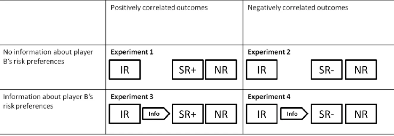
The second study deals with simple risks stemming from lotteries where probabilities are known, aiming at a better understanding of how risk taking changes if a second, passive player is affected, and if risk taking is influenced by information about other players’ decision making.⁴ In studying the effect of social preferences on risk taking, we consider a case of non-standard preferences. We measure changes in risk taking if decisions affect a second party, compare the effect of negatively and positively correlated payoffs, and vary the amount of available

3 This study is joint work with Diemo Urbig and Utz Weitzel (Stauf et al. 2011).

4 This study is joint work with Gary Bolton and Axel Ockenfels (Bolton et al. 2012).

(10)

3

information. We find that participants use the available information to adjust their risk taking, thus behaving more conform with others. Moreover, this adjustment occurs more often and to a higher degree if this implies less risk taking than before, leading to higher conservatism in a social context. The more the decisions are embedded in a social context, the more pronounced are these effects.

The third and the fourth study deal with strategic uncertainty in an n-person hero game.⁵ We investigate a situation in which exactly one person within a group should make a costly effort to increase the payoff of everyone else and reach the socially efficient outcome. In the third study, we investigate two versions of the hero game that differ with respect to their equilibria; while the first version of the game offers one equilibrium in dominant strategies in the one-shot game, the second version is a classical coordination game with n pure strategy equilibria. While behavior in the first version is largely in line with standard theory, we find that in the coordination game, a substantial fraction of players chooses strategies that should never be chosen according to standard theory. We discuss social preferences and risk aversion as potential explanations for these deviations. Furthermore, we find that players tend to behave ex- post rational; even if they are randomly rematched, they tend to adjust their behavior to their experience in the previous round. This behavioral pattern is an example of non-standard decision making.

In a follow-up study, we focus on the version of the hero game that represents a coordination problem. Probably the most common means to solve coordination problems is communication between the involved parties. We investigate the impact of two different communication mechanisms on coordination. The first mechanism allows one randomly chosen player to send a message to the other players to indicate which effort she is going to choose, which we refer to as one-way communication. The second mechanism termed multi-way communication allows all players to send messages to each other simultaneously. We show that, from a theoretical point of view, multi-way communication should not have any effect, while one-way communication

5 The third study is joint work with Christoph Feldhaus (Feldhaus and Stauf 2012) and is based on a diploma thesis (Feldhaus 2011).

(11)

4

should lead to a substantially higher coordination rate. In particular, we show that there exists an asymmetric mixed-strategy equilibrium which results in a higher expected overall payoff than the symmetric one, and we argue that it is plausible that this equilibrium is played with one-way communication. However, our experimental data shows that multi-way communication significantly improves coordination in comparison to a situation without communication, while one-way communication leads to mixed results. We propose non-standard preferences and in particular efficiency concerns as an explanation for the deviations from standard theory.

I contributed to the respective chapters in the following way. I developed the general idea for the first paper (Stauf et al. 2011, chapter 2). I designed, programmed and conducted the experiment in collaboration with Diemo Urbig. I carried out most of the statistical analyses, and I wrote the major part of the draft. Regarding the second paper (Bolton et al. 2012, chapter 3), I was centrally involved in the development of the idea and the hypotheses, as well as in the design of the experiment. I programmed and conducted the experiment, and I carried out the majority of the statistical analyses. I wrote the draft in collaboration with Gary Bolton and Axel Ockenfels.

The third paper (Feldhaus and Stauf 2012, chapter 4) is based on a diploma thesis written by Christoph Feldhaus that was supervised by Axel Ockenfels and myself; the idea for this paper came from Axel Ockenfels. I participated in the development of the hypotheses and the design.

The experiment was programmed and conducted by Christoph Feldhaus. The draft at hand is based on the text of the diploma thesis; I rewrote substantial parts and added a number of statistical analyses. The fourth paper (Stauf 2012, chapter 5) was single-authored. I developed the idea and the hypotheses based on the third paper, and I used parts of the data from the previous experiments as baseline. I designed, programmed and conducted two additional treatments, I carried out all statistical analyses, and I wrote the draft.

(12)

5

2 What is your level of overconfidence?

A strictly incentive compatible measurement method

⁶

2.1 Introduction

Overconfidence is a frequently observed, real-life phenomenon. Individuals exaggerate the precision of their knowledge, their chances for success, or the precision of specific types of information. Empirically, it has been shown that overconfidence in own performance can affect an entrepreneur's or manager's decision to enter a market (Camerer and Lovallo 1999, Wu and Knott 2006) or to invest in projects (Malmendier and Tate 2005), a stock trader’s decision to buy specific stocks (Daniel et al. 1998, Stotz and von Nitzsch 2005, Cheng 2007), or an acquirer’s decision to take over a target firm (Malmendier and Tate 2008). Lawyers' and applicants' probabilities of success are likely to depend on confidence (Compte and Postlewaite 2004), and physicians have been shown to be overconfident in their choices of medical treatment (Baumann et al. 1991). Especially the last example illustrates that the consequences of overconfidence do not only affect the decision maker, but can also have significant ramifications for third parties (e.g., patients, clients, investors, employees), as well as the economy and our society as a whole.

One stream in overconfidence research attempts to identify mechanisms that lead to overconfidence (e.g. Soll 1996, Juslin and Olsson 1997, Hilton et al. 2011). A second research stream studies how overconfidence affects evaluations of risky decision options and subsequent decisions (e.g. Simon et al. 2000, Keh et al. 2002, Cheng 2007, Coelho and de Meza 2012). A further stream of research, in which our study is embedded, is concerned with the definition and correct measurement of overconfidence.

In an early study, Fischhoff et al. (1977) consider incentives within overconfidence measurements as a potential source of measurement errors. Hoelzl and Rustichini (2005) test the effect of monetary incentives and indeed find significant differences between treatments in which participants are incentivized and those in which they are not. Despite recent advances, we

6 This study is joint work with Diemo Urbig and Utz Weitzel (Stauf et al. 2011).

(13)

6

argue that currently available mechanisms to experimentally elicit individuals’ overconfidence (e.g. Moore and Healy 2008, Blavatskyy 2009) still allow for improvements in the area of incentive compatibility and in measuring subjects’ magnitude of overconfidence more precisely.

To address these issues, we present a method of overconfidence elicitation that is strictly incentive compatible within the framework of rank-dependent utility theories, is robust to risk attitudes, and identifies different levels of overconfidence. This method does not only improve existing procedures, but also enables a direct within-subject comparison of absolute overconfidence (with respect to one’s performance) and relative overconfidence (with respect to being better than others), as both types are measured with the same methodology.

In experimentally testing this method, we provide first evidence for the importance of measuring different levels of overconfidence: We find that participants are simultaneously over- and underconfident at the population level, depending on the thresholds of relative performance. Although 95 % of participants believe to be better than at least 25 % of the population (implying overconfidence for low thresholds), only 7 % believe to be among the best 25 % (implying underconfidence for high thresholds). We argue that the application of relative thresholds that are different from the population median can provide valuable new insights. For instance, a general underconfidence to be among the best could lead to pessimism in highly competitive environments such as patent races, where investment in research and development depends on the firm’s confidence in its relative performance, or takeover auctions, where the highest bid depends on the acquirer’s confidence in realizing enough synergies to refinance the deal.

The chapter is organized as follows. The next section discusses existing methods of incentivized overconfidence elicitation and possible further improvements. In section 2.3, we present an experimental design for measuring absolute and relative overconfidence, and formally show its strict incentive compatibility. In section 2.4, we report the experimental results, compare them with the findings of previously used methods and present the characteristics of the new method.

(14)

7

Section 2.5 concludes with a discussion of limitations, future research, and possible implications of measuring levels of overconfidence.

2.2 Overconfidence measurements and potential improvements

Considering the diverse contexts in which overconfidence has been investigated, it is not surprising that various definitions of overconfidence have been used (see e.g. Griffin and Varey 1996, Larrick et al. 2007, Moore and Healy 2008, Fellner and Krügel 2011). We adopt the definition by Griffin and Varey (1996), who specify optimistic overconfidence as overestimating the likelihood that an individual’s favored outcome will occur. For reasons of legibility, we refer to optimistic overconfidence simply as overconfidence. We particularly focus on the overestimation of own performance in a knowledge-based task, which can relate to achieving an objective standard of performance (absolute overconfidence) or to be better than others (relative overconfidence).

2.2.1 Incentive compatibility

Already in 1977, Fischhoff et al. raise doubts on whether participants in overconfidence studies are sufficiently motivated to reveal their true beliefs and therefore introduce monetary stakes.

Hoelzl and Rustichini (2005) report significant differences depending on whether participants received additional incentives for predicting their performance correctly. While most overconfidence measurements implicitly assume that participants maximize their performance, optimizing the predictability by deliberately giving false answers could also be an option, especially when participants are paid for their precision in prediction. To incentivize participants to maximize their performance, Budescu et al. (1997) and Moore and Healy (2008) provide additional monetary payoffs for correctly solved quiz questions. This, however, implies a tradeoff between maximizing performance and maximizing predictability.

In Budescu et al. (1997) and Moore and Healy (2008), the payoff is calculated by means of the quadratic scoring rule (Selten 1998), the most widely used instantiation of so called proper

(15)

8

scoring rules (Savage 1971).⁷ However, the proper scoring rules also have some disadvantages.

First, they are rather complex to explain, especially if subjects do not have a sound mathematical background. Second, proper scoring rules are not robust to variations in risk attitudes (Offerman et al. 2009). Participants with different risk attitudes will provide different responses even if they hold the same belief. Recent research on individuals’ beliefs to be better than others has suggested alternative methods to elicit (relative) overconfidence, some of which can also be applied to elicit confidence in (absolute) performance. Moore and Kim (2003) provide participants with a fixed amount of money and allow them to wager any fraction of their endowment on their performance. While this method has the advantage of avoiding tradeoffs between maximizing performance and predictability and could be perceived as simpler than proper scoring rules, it is not robust to risk attitudes either. The more risk averse a participant is, the less she wagers, which confounds the measurement of the participant’s belief with his or her risk attitude.

While Moore and Kim’s (2003) investment approach is principally a trade-off between a safe income and a risky income, Hoelzl and Rustichini (2005) and Blavatskyy (2009) suggest eliciting overconfidence by implementing a trade-off between the performance risks and a lottery with predetermined odds. Hoelzl and Rustichini utilize this idea for measuring relative overconfidence by letting participants choose between playing a fifty-fifty lottery and being paid if they are better than 50 % of all participants. Blavatskyy measures absolute overconfidence in answering trivia questions and lets participants choose between being paid according to their (unknown) performance and playing a lottery. The first option results in a fixed payoff M if a randomly drawn question has been answered correctly; the second option yields the same payoff M with a probability that equals the fraction of questions that have been answered correctly, rendering the expected value of both options equivalent. The third option is to explicitely state indifference between the first and second option, leading to a random choice between both. Participants choosing the lottery are considered underconfident; those that

7 Participants receive a fixed amount of money if they perfectly predict the outcome, while the payoff is reduced by the square of the deviation if the prediction is not correct. This provides a strong incentive to come as close as possible to the true value, independent of how certain one is.

(16)

9

choose to be paid according to their performance are considered overconfident. If they indicate indifference between both alternatives, they are considered well-calibrated. This method has empirically been found to be robust to risk attitudes (Blavatskyy 2009) and, as the method by Hoelzl and Rustichini, has the elegant feature of incentivized performance maximization and elicitation of true beliefs at the same time.

The methods of Hoelzl and Rustichini (2005) and Blavatskyy (2009) as well as the revelation mechanism by Karni (2009) used by Coelho and de Meza (2009) can be considered as instances of what Offerman et al. (2009) call measuring canonical probabilities, and what Abdellaoui et al.

(2005) label the elicitation of choice-based probabilities. These procedures aim at eliciting an individual’s belief about the probability of a binary random process with payoffs H and L by determining a probability for a binary lottery with the same payoffs H and L such that individuals are indifferent between the random process and the lottery. These methods have theoretically been shown to be robust to risk attitudes in the framework of Expected Utility Theory (Wakker 2004), supporting Blavatskyy’s empirical finding. We therefore consider these methods as an excellent basis for further improvements.

Incentive compatibility in Blavatskyy’s design is based on the assumption of epsilon truthfulness, which states that participants tell the truth when there is no incentive to lie (Rasmusen 1989, Cummings et al. 1997). If subjects are well-calibrated and thus indifferent between choosing to be paid according to their performance and being paid according to a lottery, then Blavatskyy’s design expects participants to truly and explicitly indicate that indifference. Without the assumption of epsilon truthfulness, any distribution of overconfident, underconfident, and well- calibrated measurements could be explained by a population of well-calibrated participants who choose randomly in case of indifference, leading to a potential understatement of the fraction of well-calibrated subjects. To circumvent this problem, we propose an experimental design that is strictly incentive-compatible without the assumption of epsilon truthfulness.

(17)

10

2.2.2 Precision and comparability of confidence measurements

The methods suggested by Hoelzl and Rustichini (2005) and Blavatskyy (2009) only reveal whether or not a belief exceeds a certain threshold. Hoelzl and Rustichini (2005) can show that a participant believes to be worse or better than 50 % of all participants, but not whether she believes to be better than any other percentage. In Blavatskyy (2009), subjects are classified as overconfident, underconfident, or well-calibrated, but it is not possible to state whether one is more or less overconfident than another within the categories. Hoelzl and Rustichini consider a population as overconfident if more than 50 % believe to be better than 50 %. We argue that this classification does not necessarily generalize to other levels of performance. In the following, we discuss an experimental design that allows us to plot a total of ten levels of a population’s relative confidence in a range from 5 to 95 % to investigate this proposition.

In addition to measuring overconfidence and underconfidence at more levels, the method also allows a direct comparison between absolute and relative overconfidence by measuring both with the same method. This enables new empirical tests in an ongoing theoretical debate. Moore and Healy (2008) propose a theory based on Bayesian updating that explains why individuals who are overconfident also believe that they perform below average, and those who are underconfident believe that they perform above average. Larrick et al. (2007) argue that relative and absolute confidence, both being part of corresponding overconfidence measures, essentially represent subjective ability as a common underlying factor. Our experimental test thus represents a first step toward such a comparison of absolute and relative confidence.

2.3 Characteristics of the proposed method

In an attempt to improve the measurement of overconfidence along the lines discussed above and building on the methods by Hoelzl and Rustichini (2005) and Blavatskyy (2009), we propose a method that elicits canonical probabilities based on binary choices. Subjects choose repeatedly between being paid according to own performance (success or failure) and participating in a lottery with a given winning probability.

(18)

11

By selecting an appropriate set of choices, that is, levels of winning probabilities for the lotteries, our measurement method classifies participants as well-calibrated if their confidence level is closer to the actually realized performance than to any other possible performance level.

Thereby, we remove the need for well-calibrated participants to explicitly indicate their indifference. Furthermore, it provides a more robust strategy for identifying well-calibrated people in conditions where the realized performance is subject to randomness.

Assume that a participant is well-calibrated, which means that her confidence is equal to the expected performance. As long as the tasks involve a stochastic component, i.e. include imperfect knowledge, the realized performance is a random variable represented by a distribution with a mean mirroring the expected performance of a person. The values that the realized performance can take are determined by the number of tasks solved. If performance is drawn from a continuous distribution, then the probability that a participant's true expected performance matches the realized performance approaches zero. Thus, a well-calibrated participant will not be classified as such.

Furthermore, we suggest to measure performance and confidence with the same level of precision. Coelho and de Meza (2012) measure forecasting errors in subjectively expected probability to complete a skill-based task. While ten levels of confidence are elicited, the performance measure can only take the values 0 or 1, since there is only one task to be solved.

Subjects are considered optimistic if confidence exceeds realized performance. We argue, however, that if expected performance is smaller than or equal to 0.5, the closest possible realization is 0; therefore, a subject who does not succeed in the task is well-calibrated for any confidence in own performance smaller than or equal to 0.5. A more accurate classification can be achieved by increasing the number of tasks and, thereby, the number of potential realizations of performance.

To elicit degrees of overconfidence, we ask participants for multiple binary choices, one of which is randomly selected to determine the payoff (random lottery design). This method can be applied to various definitions of performance. We exemplify this by eliciting performance beliefs

(19)

12

with respect to two different types of performance, absolute and relative. Both are based on participants’ answers to ten quiz questions with an equivalent level of difficulty. For absolute performance, a participant succeeds if she answered one particular quiz question correctly and fails otherwise. This question is determined randomly. For relative performance, a participant succeeds if she answered more questions correctly than another randomly assigned participant who answered the same questions and fails if she answered fewer questions.⁸ If both answered the same number of questions correctly, one is randomly considered to have succeeded and the other to have failed.

2.3.1 Experimental design

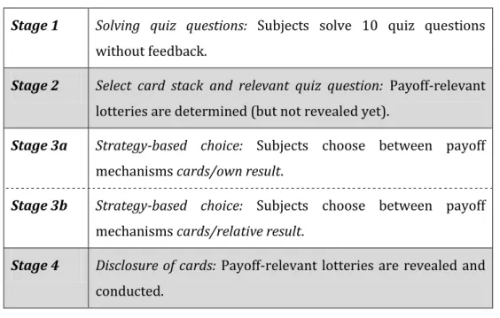
The experiment consists of four stages. The instructions can be found in Appendix A. Before starting the experiment, subjects had to pass a test for understanding the instructions. Figure 1 illustrates the course of the experiment.

Stage 1: Solving quiz questions: As usual in overconfidence experiments, participants solve ten quiz questions without feedback. For this experiment, we used multiple choice questions with four possible answers. To ensure a homogeneous level of difficulty, we started with a larger set of questions used by Eberlein et al. (2006) and selected those questions that were correctly answered by 40 to 50 % of the participants. This resulted in 28 questions, of which we then randomly selected ten questions for sessions of our experiment (question list in Appendix C).

Stage 2: Select card stack and relevant quiz question: The experimenter presents 10 stacks of 20 cards each, containing 1, 3, 5, ..., 17, 19 cards with a green cross (wins) and a complementary number of white cards (blanks).⁹ Participants do not see the number of cards with green crosses (henceforth, ‘green cards’) and do not (yet) know the distribution of green cards. One participant

8 We do not directly translate the absolute performance measurement into the relative measurement, because this requires participants to elicit their belief about the probability that they have a higher probability to be correct compared to other participants, which is rather complicated to communicate. We therefore ask them to compare the number of correct questions. As the number of correct questions is the best estimate of the probability to be correct, the direct and the indirect measure we use for the absolute and relative performance are, in fact, equivalent.

9 Note that for the method to be incentive-compatible, it is necessary to ensure that the lowest winning probability of the random mechanism (here: 5 %) is strictly lower than the minimum success probability in the task (here: 25 %). See p. 20 for a detailed explanation.

(20)

13

randomly chooses one stack; all other stacks are removed. The same procedure is repeated for a second set of stacks. Finally, one participant draws one card out of a third stack of 10 (numbered from 1 to 10) that determines the question that counts for the absolute performances of all participants.

Figure 1: Course of the experiment

Stage 1 Solving quiz questions: Subjects solve 10 quiz questions without feedback.

Stage 2 Select card stack and relevant quiz question: Payoff-relevant lotteries are determined (but not revealed yet).

Stage 3a Strategy-based choice: Subjects choose between payoff mechanisms cards/own result.

Stage 3b Strategy-based choice: Subjects choose between payoff mechanisms cards/relative result.

Stage 4 Disclosure of cards: Payoff-relevant lotteries are revealed and conducted.

Stage 3: Strategy-based choice: In a first step, participants choose between being paid according to their absolute performance and drawing a card from stack one. In a second step, they choose between being paid according to their relative performance and a card from stack two.

Participants thus choose twice between two payoff schemes, one of which is always a random mechanism. At that time, they do not know the number of green cards in the stack that was previously selected in Stage 2. However, we allow participants to condition their choice, as shown on the screenshot in the appendix and in the following example of their response: “If there are 5 green and 15 white cards in the stack and I have the choice between ‘cards’ and ‘quiz - own results,’ I choose ...,” followed by a choice between ‘cards’ and ‘quiz - own results.’¹⁰ This mechanism mirrors the strategy method introduced by Selten (1967). To control for potential

10 Rationally, for an increasing number of green cards participants should never choose “performance”

once they have chosen “cards” for less green cards. For a single person, a sequence ended with

“performance,” “cards,” “performance.” This “cards” choice was considered as “performance.”

(21)

14

order effects, one half of the participants complete the two steps in reverse order, i.e., relative performance first and absolute performance second.

Stage 4: Disclosure of cards and application of participants’ strategies: In a last step, the number of green cards in the two stacks and the number of the relevant question are disclosed.

Participants who chose to draw a card from any of the two stacks can individually draw a card.

Payoffs are calculated and individually paid to participants.

2.3.2 Measurements

Our experimental design provides us with the following individual measurements:

Absolute performance p equals the fraction of correctly answered questions.

Relative performance rp is defined as 1 if one participant was better than the other randomly assigned participant, 0 if she was worse, and 0.5 if she solved as many question as the other.

Confidence c in own absolute performance is the mean of both the highest probability for cards for which a participant would choose the absolute performance-based payoff rule and the lowest probability for cards for which a participant would choose the draw of a card from the stack of cards.

Relative confidence rc in relative performance is the mean of both the highest probability for which a participant would choose the relative performance-based payoff rule and the lowest probability for which a participant would choose the draw of a card from the stack of cards.

Absolute overconfidence oc is the difference between absolute confidence and absolute performance, oc = c - p. We consider participants as well-calibrated when overconfidence oc equals zero. Note that c is an approximation of a participant’s confidence, and the exact value of participants confidence lies in the closed interval between c=-0.05 and c=+0.05. As shown below, participants are well-calibrated when their confidence is closer to their performance than to any other possible performance.

Relative overconfidence roc is computed analogously to oc: roc = rc - p.

(22)

15 2.3.3 Formal proof of strict incentive compatibility

Applied to belief elicitation methods, incentive compatibility describes the fact that a participant is confronted with incentives that make her reveal her true belief. Strict incentive compatibility implies that revealing the truth is always strictly preferred such that any deviation results in lowering the overall value associated with an individual’s decisions. In contrast, weak incentive compatibility implies that she cannot improve her situation by not revealing the truth (Rasmusen 1989). Thus, asking individuals for their beliefs without providing any incentives against lying is weakly, but not strictly incentive compatible.

Before we report the results of the experimental test, we formally show that the proposed method is strictly incentive compatible and that it has the following properties. First, participants prefer a higher performance over a lower one, that is, they maximize their performance. Second, participants choose the lottery if the winning probability of the lottery is at least as high as their believed performance. Third, a participant is considered well-calibrated if her performance expectation is closer to the actually realized performance than to any other possible performance. This third property improves the robustness of classification of people as well-calibrated. Fourth, elicited probability judgments and resulting classification as overconfident, underconfident, or well-calibrated are theoretically robust to risk attitudes.

In order to formally show the incentive compatibility, it is necessary to make assumptions about the participants’ behavior in the form of a descriptive decision theory. For the sake of generality, we apply the cumulative prospect theory (CPT) by Tversky and Kahneman (1992), although the following proof also holds for standard expected utility theory.¹¹ Since CPT does not explicitly consider compound lotteries, i.e., lotteries over lotteries (used in our experiment), we need to include the reduction axiom as an additional assumption, which states that participants can reduce compound lotteries to their simple representation.¹²

11 See p. 21 for a detailed explanation.

12 This axiom has been challenged with respect to its empirical justification, particularly in connection with the use of random lottery mechanisms. However, empirical studies conclude that “experimenters can

(23)

16

The proof will be applied to the specific design we use in our experiment, including the double elicitation of (absolute) confidence and relative confidence. With marginal adjustments, the proof also holds if the two types of confidence are considered individually.

Participants are confronted with N choices for each of the two elicited confidences; N determines the precision. In our specific case, N equals 10. Without loss of generality, let ca,i  with 1≤i≤N be the participant’s choice between being paid according to own performance and the lottery i with winning probability pLi . In our case, the lottery i is characterized by 2i-1 winning cards among the total of 2N cards (in our case, it is 20 cards); thus, pLI=(i-0.5)/N. If the task is chosen (and not the lottery), ca,i equals 1, otherwise 0. Let cr,i  be the same for the choices between relative performance and a lottery. Vectors ca = ( ca,1, ca,2,… , ca,N) and cr = ( cr,1, cr,2,… , cr,N) represent vectors of these decisions. Furthermore, let q be the performance expectation by the participant. Let us assume that the ex-ante performance of the participant varies between qmin

and qmax, i.e qmin ≤ q ≤ qmax (depending on the participant’s choice and ability to influence the own performance). Let us further assume that the expectation of the relative performance rq is a strictly monotonic function of the performance expectation, that is, the first derivative of rq’(q) is strictly larger than 0. Let H be the amount of money that can be won in the lottery or earned when the task (absolute or relative) has been performed successfully. If the lottery is lost or the task has not been performed successfully, then participants earn nothing. As participants are assumed to follow cumulative prospect theory, the preference value V for a given set of decisions (ca, cr, q) is given by (1), with p being the belief about the occurrence of payoff H. The function v(x) represents the CPT value function applied to payoffs with v(0) = 0. For simplicity, we also assume that v(x) > 0 for x > 0. The function (p) represents the CPT probability weighting function with (p)[0,1]. Both functions are assumed to be monotonically increasing in the payoff x and the probability p, respectively.

(1) continue to use the random-lottery incentive mechanism” (Hey and Lee 2005, p. 263). Their results are supported by several other studies, for instance Starmer and Sugden (1991) and Lee (2008).

(24)

17

Applying the reduction axiom, a participant is assumed to form a belief about the occurrence of H depending on her decisions, and she is able to reduce compound lotteries to their simple representation. This is necessary as our method implements a random choice between alternatives that are themselves uncertain. Since each of the 2N (in our case 20) choices between the absolute respectively relative performance and a lottery can become relevant with equal probability, the probability for H is the average of the probabilities of all single decisions (ca,1 to ca,N and cr,1 to cr,N). As shown in Equation (2), for a single decision (between absolute performance and lottery with winning probability pLi) the probability is determined by ca,i q + (1- ca,i) pLi, which is q if the performance is chosen and pLi if the lottery is chosen. For the choice between relative performance and a lottery, the probability of a payoff H is determined correspondingly.

(2)

Note that V(ca,cr,q,H) is always larger than or equal to zero. Equation 2 can be simplified to

with

with the following derivatives with respect to the decision variables:

The terms v(H) and ’(p) are by definition strictly positive. Given that rq’(q) is strictly larger and c1i and c2i are never less than 0, we can conclude that the preference value is strictly increasing in q as long as at least one decision is made in favor of being paid according to own absolute or

(25)

18

relative performance, i.e., at least one ca,i or cr,i equals 1. In our mechanism, this is the case if the belief about own performance or the belief about relative performance is greater than 5 %.

Below this threshold, being paid according to own absolute or relative performance is never chosen, and thus there is no strict incentive to maximize this performance, i.e., the first derivative is zero. However, the minimal expected probability of success with respect to absolute performance in our experiment is 25 % (random choice out of four answers per question) such that the belief about own performance always lies above 5 %. Hence, a participant always maximizes her performance expectation.¹³

Furthermore, the preference value is strictly increasing in the decisions cx,i for x being a or r, if q respectively rq(q) are greater than the winning probability of the alternative lottery. Thus, participants will always choose the task if their belief to have succeeded is greater than the probability to win the lottery. Participants therefore always reveal their true beliefs through their choice behavior. If they do not choose the lottery for lottery i but for i+1, then the best estimation of the participant’s belief is (pLi + pLi+1)/2, which in our case is i/N.

Note that participants with a confidence between i/N-0.05 and i/N+0.05 are all classified to have a confidence level of i/N. Such participants are considered well-calibrated if they have solved i out of N tasks correctly. Therefore, even if their confidence level differs only slightly from the elicited performance, they will still be classified as well-calibrated. This holds as long as the difference between confidence and actual performance does not exceed 1/2N, which is equivalent to the condition that confidence is closer to a different level of performance that could be elicited.

All results above are based on CPT and the reduction axiom. As such, they are independent of an individual’s risk attitude as long as it satisfies the axioms of CPT. Our results are thus theoretically robust to variations in risk attitudes, modeled via value and probability weighting functions with characteristics following CPT.

13 Note that when excluding the elicitation of confidence in absolute performance such a lower threshold for performance expectations is not present.

(26)

19

The proof also holds for expected utility theory (EUT). We assume that the CPT probability weighting function (p) is monotonically increasing in p, which includes (p) = p, i.e. the absence of probability weighting. Along the same lines, any strictly increasing utility function u(x) can be linearly transformed to satisfy the assumptions imposed on the value function v(x).

2.4 Results

We conducted the experiment in two sessions with 31 female and 29 male students from University of Jena, Germany. We recruited students from all disciplines, ranging from the Natural to the Social Sciences, with the exception of Psychology. On average, the experimental session lasted 60 minutes, and participants earned 11.10 Euro.

Table 1: Descriptive statistics (mean, standard deviation, mode) and selected correlations Descriptive statistics Correlations

  median p c rc

Performance p 0.497 0.181 0.5 - 0.472 0.475

Relative performance rp 0.500 0.441 0.5 0.551 0.491 0.388

Confidence c 0.492 0.172 0.5 0.472 - 0.728

Relative confidence rc 0.498 0.173 0.5 0.475 0.728 -

Overconfidence oc -0.005 0.182 0.00 -0.551 0.476 0.215

Relative overconfidence roc¹⁴ -0.002 0.407 0.05 -0.395 -0.223 0.005 Sample size n=60

Table 1 provides some summary statistics for our experiment. The average absolute performance p is 0.497 with a median of 0.5. On average, participants have a confidence in their performance of 0.493 with median 0.5 and a confidence in their relative performance of 0.498 with a median 0.5.¹⁵ In this experiment, the participants are thus, on average, well-calibrated in absolute and in relative terms. On an individual basis, we find that 23 % of the subjects are well- calibrated, while 40 % are underconfident and 37 % are overconfident. The fraction of well- calibrated subjects is significantly higher in our setting than in Blavatskyy’s (2009) study, a fact that we ascribe to our avoidance of epsilon-truthfulness as well as applying a more robust

14 There are 30 cases with roc less than or equal to 0.00 and 30 cases greater than or equal to 0.10; thus, 0.05 is by definition the median, despite the fact that this value could not be chosen.

15 One participant violated the basic principle that the probability to win in a multiple choice task with four alternatives is at least 25% if an individual tries to maximize her performance. The behavior of this person who switched between 5% and 15% is not captured by the theories applied here. Since results do not change qualitatively, we kept this data point in the data set.

(27)

20

strategy for identifying well-calibrated participants as discussed above.¹⁶ We did not find any order effects; the order of elicitation of absolute and relative confidence did not cause significant differences.

Table 1 also reports the correlation of variables with performance p, and with confidence regarding absolute and relative performance. We find that (absolute) performance and relative performance are positively correlated, as intuitively expected, because participants with a higher performance have a greater chance to be better than others. Participants are partially aware of their performance as their (absolute) confidence and relative confidence in their performance increases with their performance (Pearson correlations are significant at the 5 % level). However, (absolute) overconfidence and relative overconfidence in performance both decrease with the level of their performance.¹⁷ This result is consistent with prior findings in overconfidence studies. Moore and Healy (2008) argue that, with higher performance, participants tend to become less overconfident and even underconfident, but at the same time believe to be better than others. While the theory by Moore and Healy tentatively suggests a negative correlation between relative confidence rc and overconfidence oc, we find a positive relation in our data.

2.4.1 Simultaneous over- and underconfidence at the population level

Above we argued for a more precise measurement of several levels of over- and underconfidence, instead of focusing on a binary belief to be better or worse than the average of a population, because an optimistic better-than-average belief may not generalize to an optimistic better-than-top 5 % belief.

Figure 2 addresses this question by plotting the relative frequency of participants who believe to be better than 5, 15, 25, …, and 95 %. Consistent with our conclusion from considering the

16 Based on a Chi-square test, we find that the two binary distributions of well-calibrated versus not well- calibrated participants are significantly different at the five percent level.

17 To better understand the relation between correlations involving overconfidence oc=c-p and relative overconfidence roc=rc-rp, on one side, and statistics about the constituent terms, c, rc, p, and rp, on the other, we refer the reader to Appendix A in Larrick et al. (2007), which provides a formal analysis of correlations with one variable being used to calculate the second variable in that correlation.

(28)

21

population average of relative confidence, approximately 50 % believe to be better than 50 % of all participants.

Figure 2: Population’s better-than-others beliefs

Thus, regarding this benchmark the group of our participants is neither over- nor underconfident. However, considering other benchmarks, the conclusion differs. About 95 % of all participants believe not to be among the worst 25 %, implying overconfidence; but only about 7 % believe to be among the best 25 %, implying underconfidence. Our group of participants is therefore underconfident for high and overconfident for low thresholds.

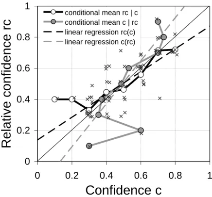
2.4.2 Confidence in absolute versus relative performance

In our experiment, we used the same methodology to elicit confidence in own absolute performance (confidence) and confidence in own relative performance (relative confidence) at the same time. This enables a direct comparison of the two types of confidence. A correlation of 0.728 (see Table 1) already indicates that both are closely related. Figure 3 visualizes the relation between both variables. Besides plotting the data points, it provides conditional means and a fitted linear approximation of the relation between both variables. As both are subject to measurement errors, conditional means as well as simple regression analysis yield biased

0 0.2 0.4 0.6 0.8 1

Performance threshold t

Relative frequency of c>t

Well-calibrated

Underconfidence Overconfidence

(29)

22

results; especially the slope of the fitted linear function might be attenuated.¹⁸ However, running a direct regression (Variable 1 on Variable 2) and a reverse regression (Variable 2 on Variable 1), as illustrated in Figure 3, provides bounds on the true parameter (Wansbeek and Meijer 2000). Despite one outlier with little relative confidence but more or less average (absolute) confidence, Figure 3 shows an interesting relation between confidence and relative confidence.

In fact, we cannot reject the hypothesis that both are identical for our data. Although this identity might not be observed in experiments where the average performance is not 50 %, we would nevertheless expect a close relation of both constructs, albeit at a different level.

Figure 3: Comparison of confidence regarding absolute and relative performance (including conditional means and linear regressions)¹⁹

18 For an in-depth discussion of the consequences of measurement errors for overconfidence research, see Erev et al. (1994), Soll (1996), Pfeifer (1994), Brenner et al. (1996), and Juslin et al. (2000).

19 To improve the visibility of data points, we added some small white noise to single data points (but not to the data used for conditional means and regressions).

0 0.2 0.4 0.6 0.8 1

Confidence c Rela tiv e co nf id en ce r c

conditional mean rc | c

conditional mean c | rc linear regression rc(c) linear regression c(rc)

(30)

23

2.5 Conclusions

This study has been motivated by the ongoing discussion about the appropriate measurement of overconfidence and, in particular, how to elicit overconfidence in strictly incentive compatible experiments. We propose and test an experimental design that adapts the advantages of the existing mechanisms, but adds several desirable features. We show that it is strictly incentive compatible within the framework of CPT (including EUT), identifies those participants as well- calibrated whose confidence is closer to their actual performance than to any other possible performance, is suited to measure overconfidence at more than a maximum of three levels (overconfidence, underconfidence, and well-calibrated confidence), and can be used to measure and compare both absolute and relative confidence.

It should be noted that the precision of performance elicitation is driven by the parameter N describing the number of binary choices used to elicit confidence beliefs. Increasing N also increases the precision of both confidence and performance measurements, which subsequently decreases the probability to identify a well-calibrated participant as such. We therefore recommend analyzing overconfidence with a range of degrees of confidence instead of dichotomous or trichotomous classifications based on single thresholds. This dependency on precision also needs to be considered when comparing results of different studies.

A general limitation concerns the common assumption that risk attitudes are independent of the source of risk. Empirical work seems to suggest that risk attitudes differ for both sources of risk, own performance, and lotteries (Heath and Tversky 1991, Kilka and Weber 2001, Abdellaoui et al. 2011). This issue clearly calls for more research into belief elicitation under conditions of source-dependent risk attitudes.

Besides the methodological advance, this paper also provides applied results. Research on relative overconfidence generally focuses on the belief to be better than the average of a population. We argue that for many social and economic situations the belief to be better than average is of less relevance than the belief to be the best or among the best. Since our mechanism elicits degrees of overconfidence, we can test whether, for instance, more than 10 %

(31)

24

of participants believe to be better than 90 %. In fact, our analysis (visualized in Figure 2) shows that, simultaneously, too few participants believe to be among the best while too many believe not to be among the worst. This may have significant economic implications, which would be worthwhile to investigate in more depth.

(32)

25

2.6 Appendix

A: Instructions for participants

There were two versions of the instructions. Both versions differ with respect to the order of treatments. In the version reported below, the first set of decisions is related to own performance while the second set of decisions is related to own relative performance. In the second, unreported version, the order is reversed.

Welcome to our experiment!

General information

You will be participating in an experiment in the economics of decision making in which you can earn money. The amount of money you will receive depends on your general knowledge and on your decisions during the experiment. Irrespective of the result of the experiment, you will receive a show-up fee of €2.50. Please do not communicate with other participants from now on.

If you have any questions, please refer to the experimenters. All decisions are made anonymously.

You will now receive detailed instructions regarding the course of the experiment.

It is crucial for the success of our study that you fully understand the instructions. After having read them, you will therefore have to answer a number of test questions to control whether you understood them correctly. The experiment will not start until all participants have answered the test questions.

Please read the instructions carefully and do not hesitate to contact the experimenters if you have any questions.

(33)

26 Course of the experiment

After all participants have read the instructions and answered the test questions, we will begin with the first part of the experiment.

In this part, you will see a sequence of 10 questions, for each of which you will have to choose 1 out of 4 possible answers. One other player in this room will be randomly assigned to you and will have to solve exactly the same series of questions.

In (the following) parts 2 and 3, we will offer you the opportunity to choose a payoff mechanism.

A payoff mechanism is a method that describes how your payoff will be determined. In both parts, 2 and 3, you will have to choose between two Options: cards or quiz.

1. Cards

For this mechanism, 20 playing cards will be shuffled. A certain number of these cards bear a green cross. You will draw one card from the stack. If it bears a green cross, you receive €7. If it does not bear a green cross, you receive €0. By the time you have to decide for or against this payoff mechanism, you will know exactly how many of the cards in the stack bear a green cross.

2. Quiz

If you choose this mechanism, your payoff depends on your answers to the quiz questions. The more questions you have answered correctly, the higher is your chance of receiving a payoff of

€7. There are two variants of the payoff mechanism “quiz”: own result and relative result.

Own result: One out of the 10 quiz questions will be drawn randomly. If you answered this question correctly, you receive a payoff of €7. Otherwise, you receive €0. With this payoff mechanism, your payoff will only depend on your own performance.

Relative result: If you answered more questions correctly than the player that has been assigned to you in the beginning and had to answer exactly the same questions, you receive €7. If you answered fewer questions correctly, you receive €0. In case of a draw, it will be randomly decided who receives the €7.

(34)

27

In the second part of the experiment, you will be able to choose between the payoff mechanisms (1) cards or

(2a) quiz – own result.

In the third part of the experiment, you will be able to choose between the payoff mechanisms (1) cards or

(2b) quiz – relative result.

In both parts, one of your options will be to draw a card from a stack which might bear a green cross, which is a pure random mechanism. The other option will always be a payoff mechanism, which determines your payoff based on your result from answering the quiz questions. This means that, in any case, you should try to correctly answer as many questions as possible. It may happen that the number of cards with a green cross is always so small that you may prefer to be paid according to your answers. In this case, your chances are better the more questions you answered correctly.

The diagram below shows the course of the experiment schematically:

Part 1 Answer quiz questions Part 2 Choose a

payoff mechanism

(1) Cards or

One out of 20 cards is drawn Green cross: €7

No green cross: €0 (2a) Quiz –

own result One quiz question is randomly drawn Correct answer: €7

Wrong answer: €0 Part 3 Choose a

payoff mechanism

(1) Cards or

One out of 20 cards is drawn Green cross: €7

No green cross: €0 (2b) Quiz –