Surface Diffusion Flow of Triple Junction Clusters in Higher Space Dimensions

Surface Diffusion Flow of Triple Junction Clusters in Higher Space Dimensions

Dissertation zur Erlangung des Doktorgrades der Naturwissenschaften (Dr. rer. nat.)

der Fakult¨ at f¨ ur Mathematik der Universit¨ at Regensburg

vorgelegt von

Michael G¨ oßwein

aus Regensburg

im Jahr 2018

Die Arbeit wurde angeleitet von: Prof. Dr. Harald Garcke (Universit¨ at Regensburg) Pr¨ ufungsausschuss: Vorsitzender: Prof. Dr. Clara L¨ oh

Erst-Gutachter: Prof. Dr. Harald Garcke

Zweit-Gutachter: PD Dr. habil. Mathias Wilke

weiterer Pr¨ ufer: Prof. Dr. Helmut Abels

Contents

1 Introduction 9

2 Preliminaries 13

2.1 Notation Conventions . . . . 13

2.2 Some Important Results from Functional Analysis . . . . 14

2.3 Function Spaces on Manifolds . . . . 15

2.3.1 Sobolev-Spaces on Manifolds . . . . 15

2.3.2 Parabolic H¨ older-Spaces on Manifolds . . . . 18

3 Short Time Existence for the Surface Diffusion Flow of Closed Hypersurfaces 21 3.1 Surface Diffusion as Gradient Flow . . . . 21

3.2 Transformation and Linearisation . . . . 22

3.3 Analysis of the Linearised Surface Diffusion Flow . . . . 23

3.4 Analysis of the Non-Linear Problem . . . . 30

4 Short Time Existence for the Surface Diffusion Flow of Triple Junction Manifolds 35 4.1 The Model and its Physical Properties . . . . 35

4.2 Parametrisation and the Analytic Problem . . . . 37

4.3 The Compatibility Conditions and the Existence Result . . . . 41

4.4 Linearisation . . . . 42

4.5 Analysis of the Linearised Problem . . . . 47

4.5.1 Existence of a Weak Solution for the Principal Part . . . . 48

4.5.2 Schauder Estimates for the Localized System on the Boundary . . . . 55

4.5.3 Schauder Estimates for the Principal Part of the Linearised Problem . . . . 59

4.5.4 The Analysis of the Full Linearised Problem . . . . 65

4.6 Analysis of the Non-Linear Problem . . . . 66

5 Stability of the Surface Diffusion Flow of Closed Hypersurfaces 77 5.1 Technical Problems Proving a Lojasiewicz-Simon Gradient Inequality: Setting for H

-flows, Banach Space Settings, Interpolation Problems . . . . 77

5.2 Parametrisation of Volume Preserving Hypersurfaces and the Surface Energy . . . . 79

5.3 Proof of the Lojasiewicz-Simon Gradient Inequality . . . . 82

5.4 Global Existence and Convergence Near Stationary Solutions . . . . 86

6 Stability of the Surface Diffusion Flow of Double-Bubbles 91 6.1 Technical Problems Proving a Lojasiewicz-Simon Gradient Inequality: Non-local Tangential Parts, Non-linear Boundary Conditions . . . . 91

6.2 Choice of the Tangential Part . . . . 92

6.3 Parametrisation of the Set of Volume Preserving Triple Junction Manifolds . . . . 95

6.4 Variation formulas for the Parametrised Surface Energy . . . . 96

6.5 The Lojasiewicz-Simon-Gradient Inequality for the Surface Energy on Triple Junction Manifolds 98 6.6 Global Existence and Stability near Stationary Double Bubbles . . . 101

Bibliography 109

Abstract

We study the evolution of double bubbles driven by the surface diffusion flow. At the triple junction we use boundary conditions derived by Garcke and Novick-Cohen in [32] in the case of curves. These are concurrency of the triple junction, Young’s law, that fixes the angles at which the three surfaces meet, continuity conditions for the chemical potentials and balance of flux conditions. In [32], Garcke and Novick-Cohen showed also short time existence in a H¨ older setting and Arab proved in [5] stability of planar double bubbles moving due to surface diffusion flow. In this work, we generalize these results to arbitrary space dimensions. Hereby, we will first apply our techniques to closed hypersurfaces to illustrate them. The results for this situations were already proven by Escher, Mayer and Simonett in [23] but with different methods.

For the short time existence result we consider reference triple junction clusters for which each hy- persurface is a submanifold of R

of class C

. We then show that for triple junction clusters that can be described as graphs over the reference frame with a combination of a height function sufficiently small in the C

-norm and a tangential part, which is given as function in the height function, there exists a solution in the parabolic H¨ older space C

. To prove this we reduce the problem via direct mapping to a fourth order, parabolic partial differential equation on the reference frame. Hereby, the tangential part will contribute non-local terms of highest order. We then linearise the problem around the reference cluster and firstly consider only the highest order terms. For the reduced system we show existence of weak solutions with a Galerkin approach. Afterwards, we localize the equations both around points in the interior of the hypersurfaces and on the triple junction. For this problem we get well-posedness in a C

-setting using classical results from Ladyzenskaja, Solonnikov and Uralceva, cf. [38]. With compactness arguments we then identify the weak solution locally as limit of solutions of the localized problem and thus get C

-regularity for the weak solutions. Using perturbation techniques we conclude this result also for the complete linear problem.

Finally, we get our existence result for the non-linear problem using a contraction mapping argument where technical difficulties arise due to the non-local tangential part and the fully non-linear angle conditions. Uniqueness of solutions remains an open problem.

In the second part of the work we show that if the reference surface is a stationary double bubble then there is a σ > 0 such that for all initial data with C

-norm less than σ the solution constructed above exists globally in time and converges to another stationary double bubble. This is done by verifying a Lojasiewicz-Simon gradient inequality for the surface area. During this the non-local tan- gential part causes crucial problems and has to be replaced by a local one. The proof of the gradient inequality itself uses then the results of Chill, see [13, Corollary 3.11]. Afterwards, we need to show parabolic regularization of the flow using the parameter trick to get bounds in the C

-norm for arbitrary large k. With this the proof of stability can be carried out applying standard arguments.

Zusammenfassung

Wir betrachten Doppel-Blasen, die durch den Oberfl¨ achendiffusionsfluss evolviert werden. Auf der

Tripellinie verwenden wir die Randbedingungen, die von Garcke und Novick-Cohen in [32] im Kur-

venfall hergeleitet wurden. Dabei handelt es sich um die Erhaltung der Tripellinie, das Youngsche

Gesetz, welches die Winkel, in denen die drei Fl¨ achen auf einander treffen, festlegt, Stetigkeitsbedin-

gungen f¨ ur die chemischen Potentiale und die Gleichheit der Ableitungen der mittleren Kr¨ ummungen

in Richtung der ¨ außeren Konormalen. Garcke und Novick-Cohen zeigten in [32] außerdem Kurzeitexis-

tenz in H¨ olderr¨ aumen und in [5] wurde von Arab Stabilit¨ at planarer Doppel-Blasen, die sich auf Grund

von Oberfl¨ achendiffusion bewegen, gezeigt. In unserer Arbeit verallgemeinern wir diese Resultate auf

beliebige Raumdimensionen. Wir wenden unsere Methoden zuerst auf geschlossene Oberfl¨ achen an,

Simonett in [23] mit anderen Techniken gezeigt.

F¨ ur die Kurzeitexistenz betrachten wir Referenzcluster, bei denen jede einzelne Oberfl¨ ache eine Un- termannigfaltigkeit des R

mit Regularit¨ at C

ist. Wir zeigen, dass f¨ ur alle Triplelinien-Cluster, die sich mittels einer H¨ ohenfunktion, die klein genug in der C

-Norm ist, und eines Tangentialteils, der als Funktion in der H¨ ohenfunktion gegeben ist, als Graph ¨ uber dem Referenzcluster schreiben lassen, eine L¨ osung in dem parabolischen H¨ olderraum C

existiert. F¨ ur den Beweis reduzieren wir das Problem zu einer skalaren, parabolischen, partiellen Differentialgleichung vierter Ordnung auf dem Referenzcluster. Dabei liefert der Tangentialteil nichtlokale Terme h¨ ochster Ordnung. Danach linearisieren wir die Gleichungen im Referenzcluster und betrachten anfangs nur die Terme h¨ ochster Ordnung. F¨ ur dieses Problem zeigen wir die Existenz schwacher L¨ osungen mit einem Galerkinansatz.

Danach lokalisieren wir das Problem sowohl um Punkte im Inneren der Fl¨ achen als auch um Punkte auf der Tripellinie. F¨ ur die Lokalisierung erhalten wir Wohlgestelltheit in C

durch Anwendung der Resultate von Ladyschenskaja, Solonnikov und Uralceva, siehe [51]. Mit einem Kompaktheitsar- gument identifizieren wir die schwache L¨ osung lokal als Grenzwert von L¨ osungen des lokalisierten Problems und erhalten damit auch C

-Regularit¨ at f¨ ur die schwache L¨ osunge. Durch ein St¨ orungsargument folgern wir hieraus das gleiche Resultate auch f¨ ur das komplette linearisierte Prob- lem. Schließlich erhalten wir das Existenzresultat f¨ ur das nichtlineare Problem mittels des Banach- schen Fixpunktsatzes. Hierbei entstehen technische Schwierigkeiten durch den nichtlokalen Tangen- tialteil und die voll-nichtlinearen Winkelbedingungen. Eindeutigkeit f¨ ur die L¨ osung des geometrischen Flusses bleibt ein offenes Problem.

Im zweiten Teil der Arbeit zeigen wir, dass es f¨ ur Referenzcluster, die station¨ are Doppel-Blasen

sind, ein σ > 0 gibt, sodass f¨ ur alle Anfangsdaten mit einer C

-Norm kleiner oder gleich σ die

gefundene L¨ osung global in der Zeit existiert und gegen eine andere station¨ are Doppel-Blase kon-

vergiert. Hierbei nutzen wir einen Ansatz mit einer Lojasiewicz-Simon Gradientenungleichung f¨ ur

die Oberfl¨ achenenergie. Bei deren Beweis entpuppt sich der nichtlokale Tangentialteil als kritisches

Problem, weshalb er durch einen lokalen ersetzt werden muss. Die Ungleichung selbst kann dann mit

den Resultaten von Chill, siehe [13, Corollary 3.11], gezeigt werden. Danach muss parabolische Regu-

larisierung des Flusses mit Hilfe des Parametertricks gezeigt werden, um Schranken in der C

-Norm

f¨ ur beliebig große k zu zeigen. Mit diesen ist die Stabilit¨ atsanalyse mit Standardargumenten m¨ oglich.

Acknowledgements

I would like to thank everybody who supported me academically and personally in the last four years.

Without all those great people this project would not have been possible.

First and foremost, I want to thank my supervisor Prof. Dr. Harald Garcke for suggesting the topic of this thesis and supporting me in solving all arising problems during the project. He has also been my guide through my whole academic adolescence beginning from my Bachelor thesis. Prof. Dr. Gar- cke provided me with a lot of understanding and intuition for mathematics for which I am very grateful.

I would like to thank Prof. Dr. Helmut Abels who always found time to share his expertise with me. In particular, the discussions about parabolic smoothing and the parameter trick were very help- ful.

Furthermore, I want to thank Prof. Dr. Ralph Chill and PD Dr. habil. Mathias Wilke for the helpful discussions concerning the Lojasiewicz-Simon gradient inequality.

I am very grateful to all the great colleagues I had around me at the faculty. They always cre- ated an inspiring working atmosphere and I would like to name (in alphabetic order) the following who became very important to me. Tobias Ameismeier is one of the most energetic people I have ever met and him being around was always bracing. Christopher Brand inspired me with his broad knowledge and interest for mathematics and all the discussions we had. I have worked together with Dr. Julia Butz since our Master’s degree and during my time as PhD-student she was also a per- son who enabled me a lot of perceptions. Matthias Ebenbeck is the kind of reliable and perfectly balanced guy you do not want to miss as a friend. Dr. Hans Fritz was always like a mentor for me and I grew personally from our conversations. Dr. Johannes Kampmann always had a sympathetic ear for my questions and took a lot of time to discuss them. I shared a lot of research interests and ideals about good mathematics with Julia Menzel and I enjoyed working and discussing with her.

Alessandra Pluda, Ph.D., inspired me with her geometrical intuition she shared with me during a lot of nice Italian lunches. Maximilian Rauchecker was very supportive in all difficult situations and always found time for me. Felicitias Schmitz was the best office mate one could imagine and my ideas always caught fire with her. Dr. Johannes Wittmann’s unfailing joyful kind made the faculty a much warmer place for me.

I gratefully acknowledge the financial support by the DFG graduate school GRK 1692 Curvature, Cycles, and Cohomology in Regensburg. Also, I would like to thank all participating people for pro- viding an interdisciplinary community.

Last but not least, I want to thank Dr. Markus Meiringer. During high school he gave me the

first impulses for mathematics and he is still a very dear friend to me.

Introduction 1

A geometric evolution equation is a law that either describes the evolution of a geometric object or a geometric quantity of a fixed object. These kind of problems have both motivations from applications in natural sciences and mathematics. With such equations one can describe for example crystal growth (see e.g. [8]), two-phase flows of two mixed liquids (see e.g. [47]), and flame propagation (see e.g. [50]).

Also, they are used in image analysis, see e.g. [6]. Another very prominent application of geometric flows in mathematics is given by Perelman’s proof of the Poincar´ e conjecture. In his work [46], the author used the Ricci flow together with so called surgery techniques to give a complete topological characterization of simply connected, closed 3-manifolds. This shows how broad the possibilities in this subject are.

For this thesis we are interested in evolution laws that describe evolution of geometric objects. Typical examples for such are the mean curvature flow

V

= H

, (MCF)

the surface diffusion flow,

V

= −∆

H

, (SDF)

and the Wilmore flow

V

= −∆

H

− H

|II

|

+ 1

2 H

. (WF)

Hereby, Γ(t) denotes an evolving hypersurface, V

its normal velocity, H

its mean curvature,

∆

the Laplace-Beltrami operator and II

the second fundamental form. From these evolution

laws we see directly a general problem of these flows. They only fix the normal velocity and so these

problems are degenerated as motion laws for the particles of the surface. So, to get a well-posed prob-

lem of the geometric object one has to restrict freedoms in the tangential motions. In [44, Proposition

1.3.4] it is proven that for manifolds without boundary solutions of the mean curvature flow with

different tangential parts are equivalent up to reparametrisation. This result can be generalized to

general flows but things are more complicated when manifolds with boundaries are involved. Near the

boundary we cannot completely ignore tangential parts as a reparametrisation has to map boundary

points to boundary points. Before we now move to our problem we want to mention that writing

these problems in local coordinates results in quasi-linear systems which makes them more difficult

then they look at first glance.

In this thesis we study motion by surface diffusion flow. This law was first proposed by Mullins [45] in 1957 to model the motion of grain boundaries of a heated polycrystal. This was identified by Cahn and Taylor in [11] for closed hypersurfaces as H

-gradient flow of the surface energy and also linked by Cahn, Elliott and Novick-Cohen in [10] with the Cahn-Hilliard equation with degenerate mobility as its sharp-interface limit. Short time existence and stability of stationary points was dis- cussed by Elliott and Garcke in [22] for closed, planar curves and generalized to the higher dimensional case by Escher, Mayer and Simonett in [23]. Finally, we want to give an overview on some results concerning long time behaviour. For mean curvature flow one can observe typical properties linked to maximum principles. For example, Grayson showed in [34] that a smooth embedded planar curve preserves this properties and becomes convex in time. This can be combined with the work of Gage and Hamilton [26] where the authors showed that a convex curve in the plane moving due to mean curvature flow remains convex and shrinks to a round point. This is both false for surface diffusion flow as it was proven by Giga and Ito in [27, 28].

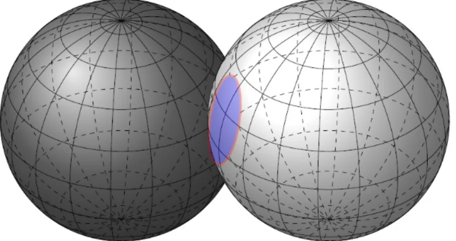
Figure 1.1: The picture shows the considered kind of triple junction cluster. In total, there are three hypersurfaces. In this illustration these are the two spherical caps and the flat blue area.

The red line marks the triple junction, which is the boundary of all three hypersurfaces.

Note that if the two enclosed volumes are unequal the blue surfaces will normally bend into direction of the larger volume.

Now we want to talk about the geometrical situation studied in this thesis. We will consider three embedded, oriented, compact, connected hypersurfaces Γ

, Γ

, Γ

in R

that do not intersect with each other. Furthermore, their boundaries coincide, that is

∂Γ

= ∂Γ

= ∂Γ

:= Σ,

and so they meet each other in a triple junction Σ. The most prominent example for this kind of geometry is the so called standard double bubble that was proven in [36] to have the best ratio between its surface area and the enclosed volume. We will now consider an evolution

Γ(t) := Γ

(t) ∪ Γ

(t) ∪ Γ

(t) ∪ Σ(t),

that fulfils at every time (SDF) and in addition on Σ(t) the boundary conditions

∂Γ

(t) = ∂Γ

(t) = ∂Γ

(t) = Σ(t), (CC)

∠ (ν

, ν

) = θ

, (i, j, k) ∈ {(1, 2, 3), (2, 3, 1), (3, 1, 2)}, (AC) γ

H

+ γ

H

+ γ

H

= 0, (CCP)

∇

H

· ν

= ∇

H

· ν

= ∇

H

· ν

. (FB)

Here, ν

denotes the outer conormal of Γ

(t), γ

, γ

, γ

constants determining the energy density on the hypersurfaces Γ

(t) and θ

, θ

, θ

∈ [0, 2π] given angles, that are actually given by the γ

. Indeed, the condition (AC) is equivalent to Young’s law

sin(θ

)

γ

= sin(θ

)

γ

= sin(θ

) γ

,

that was derived in [54] as balance of mechanical forces. The condition (CCP) results from continu- ity of the chemical potentials at the triple junction and (FB) are the flux balances. (CC) gives the concurrency of the triple junction during the flow. For the motivation of these boundary conditions as sharp interface limit of a Cahn-Hilliard equation with degenerate mobility see [32].

We will prove two main results in this thesis. The first one is short time existence in a H¨ older setting for triple junction clusters that are for some α ∈ (0, 1) close enough in the C

-norm to a C

-reference surface. Hereby, we follow the ideas from [32], which were also applied in [31]. In these works the authors linearised the problem over a fixed reference frame and then used directly the results from [38]. The non-linear analysis is then as usual based on a contraction argument using Banach’s fixed-point theorem. In our situation we get more complications due to the higher space dimensions. In contrary to curves general manifolds cannot be written as parametrisation over one domain in R

. Thus, we can apply [38] only locally and we therefore need to construct a global weak solution and connect both problems using compactness arguments. Additionally, there are three other main problems in the analysis we want to explain. Firstly, as mentioned before, we have to reduce the tangential freedom to get a well-posed problem. Hereby, we use the ideas from [19] and as a consequence we get non-local terms in highest order. The authors observed that in the linearisation of their equations all non-local terms appear only in lower order. We want to emphasise that this is natural for the linearisation in the reference frame of expressions caused by tangential terms in curvature quantities. Thus, in the linear analysis of curvature flows we do not expect non-local terms to cause technical problems in general. For the non-linear analysis the authors of [19] modify theory for fully non-linear equations from [42]. In our work, we want to show that this is not necessary and we can use directly the quasi-linear structure of the non-local terms. The second difficult aspect are the angle conditions (AC). They will lead to a fully non-linear boundary condition for which we need techniques from [42]. Also, this will cause essential problems proving parabolic smoothing. Thirdly, in the weak analysis of the linearised problem we get an energetic problem with the inhomogeneities of all lower order boundary conditions. These have to be included in the end using perturbations techniques. As final comment we want to remark that we expect that the application of maximal L

-regularity like they were used in [49] is in principle possible. But as we have boundary conditions of mixed orders we cannot apply the results directly.

The second main result of this thesis is that the evolution due to surface diffusion of triple junc-

tion clusters close to stationary double bubbles will exists globally in time. Furthermore, the flow

converges to another stationary double bubble. This was already proven in [5] for planar double bub-

bles. The author used there the generalized principle of linearised stability which is also applied in

related works. Depner proved in [16] linearised stability of mean curvature and surface diffusion flow

with boundary contact and with and without triple lines. Abels, Garcke and M¨ uller proved in [1] sta-

bility of spherical caps evolving due to Wilmore flow. A different approach was used in [23] where the

authors used centre manifold analysis to prove stability of stationary points of surface diffusion flow

on closed hypersurfaces. Both methods are difficult to apply in our situation as one needs a precise de-

scription of the set of equilibria of the flow. In [5] the author was able to give one in the case for planar

double bubbles. But there the triple junctions are only points. In higher space dimensions they itself

will be non-trivial geometrical objects causing more degree of freedoms in the set of equilibria. Thus,

we used an approach with a Lojasiewicz-Simon gradient inequality. Hereby, one uses the fact that once

such an inequality is proven we get estimates for the time derivative, cf. [14, Section 4] for a detailed

explanation. In [13] the author gave a general result concerning prerequisites for a Lojasiewicz-Simon

gradient inequality to be true. To use this in most situations a more practical version this results was

written down by Feehan and Meridakis in [25]. This method is easy to apply and was for example also

used in situations with higher codimensions, cf. [14] and [15]. In our work several aspects made the application more complicated than in the mentioned works. Firstly, most authors consider L

-gradient flows. Our problem is related to a H

-flow but the gradient flow structure itself is not clear. Thus, we have to do some modification in the stability argument. Secondly, due to the higher space dimensions one cannot work in the natural function spaces one would expect. In these spaces the geometric objects cannot guaranteed to be C

-manifolds. To solve this complicated interpolation arguments are needed.

Thirdly, the non-linear boundary conditions on the triple junctions are difficult to fit in the classical setting of [13, Corollary 3.11.]. In [15] the authors considered open curves with clamped boundaries.

This results in linear boundary conditions which are much easier in their analysis. Finally and most critical is the tangential part of the flow. During our work we realized that a non-local tangential part will not be suitable to work with and so we have to replace it later in the work with a local version.

As an outlook we want to give some examples of further questions related to the topic which are not discussed in this thesis. The short time existence results remains open for general C

-surfaces.

Here, suitable approximation results for triple junction clusters like they were proven for closed hy- persurfaces in [49] are needed. Additionally, like in many higher dimensional situations the question for existence and uniqueness for the original geometric problem remains unanswered.

Lastly, we give a brief overview concerning the structure of this thesis. In Chapter 2 we will ex-

plain basic notation used in this thesis, recall necessary results from function analysis and give an

overview of function spaces on manifolds we will use. In Chapter 3 we motivate our strategy to prove

short time existence by applying it on closed hypersurfaces. This result was already proven in [23] with

other methods. In Chapter 4 we will then use this methods on triple junction clusters. In Chapter

5 we will show stability of stationary points of surface diffusion flow on closed hypersurfaces. This

results was also already proven in [23] with other methods. Finally, we will prove stability of standard

double bubbles evolving due to surface diffusion flow in Chapter 6.

Preliminaries 2

2.1 Notation Conventions

Throughout this thesis we will work with two different kinds of time-evolving geometries: either closed (i.e. compact and without boundary), embedded, connected, orientable hypersurfaces or triple junction surface clusters of three compact, embedded, connected hypersurfaces. We will denote in both cases by Γ(t) the geometric object at time t. In the case of closed hypersurfaces we will denote by Ω the volume enclosed by Γ. In case of triple junction manifolds we will denote by Γ

, Γ

and Γ

the three hypersurfaces and by Σ(t) the arising triple junction, that is

Σ(t) = ∂Γ

(t) = ∂Γ

(t) = ∂Γ

(t).

Two of the hypersurfaces will always form a volume containing the third hypersurface, which we will choose to be Γ

. By Ω

and Ω

we denote the volume enclosed by Γ

and Γ

resp. Γ

and Γ

. We choose the normals of the hypersurfaces, which we will denote in both cases by N , such that the normal of Γ

points in the interior of Ω

, the one of Γ

outside of Ω

and the one of Γ

into the inside of Ω

. The outer conormals will be denoted by ν .

Furthermore, we use the standard notation for quantities of differential geometry, see for example [37] or the second chapter of [16]. That includes the canonical basis {∂

}

of the tangent space T

Γ at a point p ∈ Γ induced by a parametrisation ϕ, the entries g

of the metrical tensor g, the entries g

of the inverse metric tensor g

, the Christoffel symbols Γ

, the second fundamental form II , its squared norm |II|

and the entries h

of the shape operator. We use the usual differential operators on a manifold Γ, which are the surface gradient ∇

, the surface divergence div

and the Laplace-Beltrami operator ∆

(cf. [16, Section 2.1]).

By ρ we will denote the evolution in normal direction and by µ the evolution in tangential direction, which we will use to track the evolution of Γ(t) over Γ

via a direct mapping approach. Γ

resp.

Γ

will denote the (triple junction) manifold that is given as graph over Γ

, cf. (3.1) and (4.17).

Sub- and superscripts ρ resp. µ on a quantity will indicate that the quantity refers to the manifold Γ

. Hereby, we will normally omit µ as long it is given as function in ρ. An asterisk will denote an evaluation in the reference geometry. Both conventions are also used for differential operators. For example, we will write ∇

for ∇

and ∇

for ∇

. We will denote by J

the transformation of the surface measure, that is,

dH

(Γ

) = J

dH

(Γ

).

If we index a domain or a submanifold in R

with a T or δ in the subscript, this indicates the corresponding parabolic set, e.g., Γ

= Γ × [0, T ]. With an abuse of notation, in most parts of the work we will not differ between quantities on Γ

and the pullback of them on Γ

. In the parts dealing with triple junction manifolds the index i will be used to indicate that a quantity refers to the hypersurface Γ

. A quantity in bold characters will refer to the vector consisting of the quantity on the three hypersurfaces of a triple junction, e.g., ρ = (ρ

, ρ

, ρ

).

For the used function spaces we want to clarify that a subscript (0) denotes in the case of closed hypersurfaces a mean value free function and for a function ρ on a triple junction manifold Γ the condition

ˆ

Γ¹

ρ

dH

= ˆ

Γ²

ρ

dH

= ˆ

Γ³

ρ

dH

. Also, we denote by ffl

Γ

f dH

the mean value of a function f ∈ L

(Γ), that is,

Γ

f dH

:= Area(Γ)

ˆ

Γ

f dH

.

If Γ is a triple junction manifold then the subscript TJ in a function space will indicate that the function space has to be read as product space on each hypersurface. For example, we write

L

(Γ) := L

(Γ

) × L

(Γ

) × L

(Γ

).

In the chapter about stability we follow the notation of [13]. In particular, E : V → R denotes an energy functional (in our case just the surface area) on a Banach spaces V , M its first derivative and L(0) its second derivative at point 0. Hereby, we will always consider L(0) as function on V with values (on a subset of) V

.

Finally, we will always use the convention of dynamical constants. This will also be used for coefficient functions of lower order terms. The latter will be introduced in Section 4.4.

2.2 Some Important Results from Functional Analysis

During this thesis, a lot of problems will be dealt with by using the implicit function theorem for functions between Banach spaces. Therefore we want to mention the following version from [55, Theorem 4B].

Proposition 2.1 (Implicit function theorem of Hildebrandt and Graves).

Suppose that:

i.) the mapping : : U(x

, y

) ⊂ X × Y → Z is defined on an open neighbourhood U (x

, y

), and F (x

, y

) = 0, where X, Y, Z are Banach spaces over K ∈ { R , C } and x

∈ X, y

∈ Y .

ii.) ∂

F exists as a partial Fr´ echet-derivative on U(x

, y

) and ∂

F(x

, y

) : Y → Z is bijective.

iii.) F and ∂

F are continuous at (x

, y

).

Then, the following are true:

a.) Existence and uniqueness: There exist positive numbers r

and r such that for every x ∈ X satisfying kx − x

k

≤ r

there is exactly one y(x) ∈ Y for which ky(x) − y

k

≤ r and F (x, y(x)) = 0.

b.) Continuity: If F is continuous in a neighbourhood of (x

, y

), then y(·) is continuous in a neighbourhood of x

.

c.) Continuous differentiability: If F is a C

-map on a neighbourhood of (x

, y

), 1 ≤ m ≤ ∞, then y(.) is also a C

-map on a neighbourhood of x

.

For our work on stability, analyticity of functions between Banach spaces is an important concept. To

define it, we first have to introduce so called power operators.

2.3 Function Spaces on Manifolds

Definition 2.2 (Power operator).

Let X and Y be Banach spaces over K ∈ { R , C }. Let there be given a k-linear, bounded operator M : X × · · · × X → Y which is symmetric in all variables. A power operator of degree k is created from setting for all m, n ∈ {0, 1, ..., k} with m + n = k and x, y ∈ X

M x

y

:= M (x, ..., x

| {z }

mtimes

, y, ..., y

| {z }

n−times

).

Definition 2.3 (Analytic Operators between Banach Spaces).

Let Z and Y be Banach spaces over K and T : Z ⊃ D(T) → Y defined on an open set D(T ).

i.) T is called analytic at z

∈ D(T ), if there is a sequence {T

}

of power operators of degree k together with an open neighbourhood U of z

∈ D(T ) such that for all z ∈ U the series

Sz :=

∞

X

k=0

T

(z − z

)

(2.1)

exists and we have Sz = T z for all z ∈ U .

ii.) T is called analytic on an open subset V ⊂ D(T ), if it is analytic at every point z

∈ V . Remark 2.4. Note that if T is analytic at a point z

, this implies that T is analytic in an open neighbourhood of z

, cf. [55, p.98].

Very important for our work will also be that the implicit function theorem inherits also analyticity, which is Corollary 4.23 in [55].

Corollary 2.5 (Analytic version of the implicit function theorem).

If in the situation of Proposition 2.1 the function F is also analytic at (x

, y

), then the solution y is analytic at x

as well.

The last thing we want to mention is the following fact about compact perturbations of Fredholm operators, which is Proposition 8.14(3) in [55].

Proposition 2.6 (Compact perturbation of Fredholm operators).

Let X, Y be Banach spaces, B : X → Y a Fredholm operator and C : X → Y a compact operator.

Then the sum B + C : X → Y is also a Fredholm operator and the Fredholm index satisfies

ind(B + C) = ind(B ). (2.2)

2.3 Function Spaces on Manifolds

In this section we want to introduce the two most important function spaces on manifolds we will use.

These are Sobolev and parabolic H¨ older spaces. In this section, (Γ, A) will always be a compact, ori- entable, embedded submanifold Γ of R

, either with or without boundary, together with a maximal atlas A.

2.3.1 Sobolev-Spaces on Manifolds

Definition 2.7 (Sobolev spaces on manifolds). Let Γ be of class C

, j ∈ N . Then we define for k ∈ N , k < j, 1 ≤ p ≤ ∞ the Sobolev space W

(Γ) as the set of all functions f : Γ → R , such that for any chart ϕ ∈ A, ϕ : V → U with V ⊂ Γ, U ⊂ R

the map f ◦ ϕ

is in W

(U ). Hereby, W

(U ) denotes the usual Sobolev space. We define a norm on W

(Γ) by

kf k

:=

s

X

i=1

kf ◦ ϕ

k

, (2.3)

where {ϕ

: V

→ U

}

⊂ A is a family of charts that covers Γ.

Remark 2.8 (Equivalent norms on W

(Γ)).

i.) The norm on W

(Γ) depends on the choice of the ϕ

but for a different choice we will get an equivalent norm as the transitions maps are C

.

ii.) For the space W

(Γ) we will use the norm kf k

=

ˆ

Γ

|∇

f |

+ |f |

dH

. (2.4)

Equivalence to (2.3) follows directly from the representation of the surface gradient in local coordinates.

iii.) As usual we will write H

(Γ) for W

(Γ).

We want to make some further remarks on three properties of these spaces. The first one is a sufficient condition such that we get a Banach algebra structure.

Lemma 2.9 (Banach space property of Sobolev spaces).

Let Γ be smooth, k ∈ N , 1 ≤ p ≤ ∞, and assume that p > 2n

k . (2.5)

Then, W

(Γ) is a Banach algebra. In particular, H

(Γ) is a Banach algebra for k > n.

Proof. It is enough to show the result in local coordinates. So, we consider for a bounded domain V two functions f, g ∈ W

(V ). For any multi-index α with |α| ≤ k the partial derivative ∂

(f g) is due to the Leibnitz rule a sum of terms of the form ∂

f ∂

g with |α

| +|α

| = |α|. As each derivative of f and g is in L

(V ) it is enough to guarantee that W

(V ) , → C [

](V ). Using the Sobolev embedding this is true as long as (2.5) is fulfilled.

For the next two results we will consider a triple junction cluster Γ. For a differentiable manifold the Poincar´ e inequality is well known, cf. [35, Theorem 2.10]. This can also be used for each surface of Γ. But by imposing additional boundary conditions one also can guarantee a version for the whole cluster.

Proposition 2.10 (Poincar´ e-type inequality on triple junction manifolds).

Let γ

> 0, i = 1, 2, 3. Consider the space E :=

(

ρ ∈ H

(Γ)

3

X

i=1

γ

ρ

= 0, ˆ

Γ¹

ρ

dH

= ˆ

Γ²

ρ

dH

= ˆ

Γ³

ρ

dH

)

. (2.6)

Then, there is a constant C > 0 such that for all ρ ∈ E we have kρk

T J(Γ)

≤ Ck∇

ρk

T J(Γ)

. (2.7)

Proof. This was proved in [16, Lemma 4.29] for the situation with boundary contact. The proof only uses the structure at the triple junction and therefore can also be used in our situation.

For the study of weak solutions we will need an Ehrling-type lemma.

Proposition 2.11 (Ehrling-type lemma on triple junction).

For every ε > 0 there exists a C

> 0 only depending on ε such that for all u ∈ H

(Γ) it holds kuk

≤ εk∇

uk

T J(Γ)

+ C

kuk

T J(Γ)

. (2.8)

Proof. Assume by contradiction that for some ε > 0 there is a sequence ( u e

)

⊂ H

(Γ) with k u e

k

> εk∇

u e

k

T J(Γ)

+ nk u e

k

T J(Γ)

. (2.9)

2.3 Function Spaces on Manifolds

Then consider for all n ∈ N the function u

:= u e

· k u e

k

. Note that due to (2.9) this is well defined. Now, multiplying (2.9) with k u e

k

implies that

1 > εk∇

u

k

T J(Γ)

+ nku

k

T J(Γ)

. (2.10)

From this we conclude that (u

)

has to converge to 0 in L

(Γ) and that k∇

u

k

is uniformly bounded by

. Thus, (u

)

is bounded in H

(Γ) and consequently there is a subsequence (u

)

converging weakly to a u ∈ H

(Γ). Due to the compact embedding H

(Γ) , → L

(Γ) this sequence converges strongly in L

(Γ) and by uniqueness of limits this shows that u ≡ 0. Using compactness of the trace operator we see that u

also converges strongly in L

(Σ)

to 0. Now, this is a contradiction as we constructed u

to be normalized in L

(Σ)

and therefore we conclude our claim.

The last thing we want to mention concerning Sobolev spaces is the space H

. In the case of a closed hypersurface Γ this denotes the dual space of E = H

(Γ) and in the case of triple junctions the dual space of E from (2.6). As we showed above we have a Poincar´ e inequality on both spaces and therefore an equivalent inner product on these spaces is given by the L

-product of the surface gradients. Using the Riesz isomorphism we can identify the elements of H

with E, that is, for every f ∈ H

there is a unique ρ ∈ E with

ˆ

Γ

∇

ρ · ∇

ψdH

= f (ψ) ∀ψ ∈ E. (2.11)

But this is nothing else but the weak formulation of

−∆

ρ = f on Γ

, (2.12)

in the closed case and otherwise the weak formulation of

−∆

ρ

= f

on Γ

, i = 1, 2, 3, (2.13)

ρ

+ ρ

+ ρ

= 0 on Σ, (2.14)

∂

ρ

= ∂

ρ

= ∂

ρ

on Σ. (2.15)

Therefore, we will write for the element from the Riesz identification (−∆

)

f and get the inner product on H

by

hf, gi

:=

ˆ

Γ

∇

((−∆

)

f ) · ∇

((−∆

)

g)dH

, f, g ∈ H

. (2.16) We will later need the following interpolation result.

Lemma 2.12 (Interpolation between H

and H

).

Let Γ be either a closed hypersurface or a triple junction cluster. Then we have for all ρ ∈ E that kρk

≤ kρk

kρk

. (2.17) .

Proof. We will only consider the case of triple junctions as the closed case works alike without boundary terms. Using the properties of (−∆

)

and the Cauchy-Schwarz inequality we get

ˆ

Γ

ρ

dH

=

3

X

i=1

ˆ

Γ

−∆

(−∆

)

ρ

ρ

dH

=

3

X

i=1

ˆ

Γⁱ

∇

(−∆

)

ρ

· ∇

ρ

dH

− ˆ

Σ 3

X

i=1

∇

(−∆

)

ρ

· ν

ρ

dH

=

3

X

i=1

ˆ

Γⁱ

∇

(−∆

)

ρ

· ∇

ρ

dH

≤ kρk

kρk

. This shows the claimed estimate.

2.3.2 Parabolic H¨ older-Spaces on Manifolds

Now, we want to move on to the second kind of important function spaces, the parabolic H¨ older spaces. It is both possible to introduce these spaces on manifolds in local coordinates, e.g. [42, p.177], or without, e.g. [19]. We prefer the first approach as we want to use local results. We will first introduce these spaces on a bounded domain Ω in R

with smooth boundary ∂Ω. For this, we first need for α ∈ (0, 1), a, b ∈ R the two semi-norms for a function f : ¯ Ω × [a, b] → R given by

hf i

:= sup

x1,x2∈Ω,t∈[a,b]¯

|f (x

, t) − f (x

, t)|

|x

− x

|

, hf i

:= sup

x∈Ω,t¯ 1,t2∈[a,b]

|f(x, t

) − f (x, t

)|

|t

− t

|

. Now, we define for k, k

∈ N , α ∈ (0, 1), m ∈ N the spaces

C

( ¯ Ω × [a, b]) := {f ∈ C( ¯ Ω × [a, b])|hf i

< ∞}, kf k

:= kf k

+ hfi

,

C

( ¯ Ω × [a, b]) := {f ∈ C( ¯ Ω × [a, b])|hf i

< ∞}, kf k

:= kf k

+ hfi

,

C

( ¯ Ω × [a, b]) := {f ∈ C( ¯ Ω × [a, b])|∀t ∈ [a, b] : f ∈ C

( ¯ Ω),

∀β ∈ N

, |β| ≤ k : ∂

f ∈ C

( ¯ Ω × [a, b])}, kf k

:= X

|β|≤k

k∂

fk

+ X

|β|=k

h∂

f i

,

C

( ¯ Ω × [a, b]) := {f ∈ C( ¯ Ω × [a, b])|∀β ∈ N

, i ∈ N

, mi + |β| ≤ k :

∂

∂

f ∈ C

( ¯ Ω × [a, b]) ∩ C

( ¯ Ω × [a, b])}, kf k

C^k+α,k+αm ( ¯Ω×[a,b])

:= X

0≤mi+|β|≤k

k∂

∂

f k

+ k∂

∂

f k

C^0,

k+α−mi−|β|

m ( ¯Ω×[a,b])

+ X

mi+|β|=k

k∂

∂

f k

.

Hereby, we denote by ∂

a partial derivative in space with respect to the multi-index β and ∂

the i-th partial derivative in time. The parameter m corresponds to the order of the differential equation one is considering and in our work it will always be four. Now, we can also define parabolic H¨ older spaces on submanifolds as follows.

Definition 2.13 (Parabolic H¨ older spaces on submanifolds).

Let Γ be a C

-submanifold of R

, either with or without boundary. Then we define for k ∈ N

, k <

r, α ∈ (0, 1), a, b ∈ R , m ∈ N the space C

(Γ × [a, b]) as the set of all functions f : Γ → R such that for any parametrisation ϕ : Ω → V ⊂ Γ we have that f ◦ ϕ ∈ C

( ¯ Ω × [a, b]).

Remark 2.14 (Traces of parabolic H¨ older spaces).

On the boundary Σ of Γ we may choose ϕ to be a parametrisation that flattens the boundary. From this we see that

f ∈ C

(Γ × [a, b]) ⇒ f

∈ C

(Σ × [a, b]).

2.3 Function Spaces on Manifolds

Remark 2.15 (H¨ older regularity in time for derivatives).

In some works these spaces are introduced with lower H¨ older regularity in time for the lower order derivatives, cf. [42] and [19]. Actually, this approach is equivalent due to interpolation results for H¨ older continuous functions, cf. [42, Proposition 1.1.4 and 1.1.5].

The following properties are proved only in the case of parabolic H¨ older spaces on bounded domains of R

. Due to the definition in local coordinates they are also true for parabolic H¨ older spaces on submanifolds.

Like in most works on well-posedness, product estimates will also be crucial in our work. Regarding this, we have very good properties in parabolic H¨ older spaces.

Lemma 2.16 (Product estimates in parabolic H¨ older spaces).

Let k, m ∈ N , α ∈ (0, 1) and f, g ∈ C

(Ω × [0, T ]). Then we have

f g ∈ C

(Ω × [0, T ]), (2.18)

and furthermore we have that kf gk

C^k+α,k+αm (Ω×[0,T])

≤ Ckf k

C^k+α,k+αm (Ω×[0,T])

kgk

C^k+α,k+αm (Ω×[0,T])

, (2.19)

kf gk

C^k+α,k+αm (Ω×[0,T])

≤ C

kf k

C^k+α,k+αm (Ω×[0,T])

kgk

+ kf k

kgk

C^k+α,k+αm (Ω×[0,T])

. (2.20) Proof. Using again the Leibntz rule we see that all partial derivatives, that exist for f and g, exist also for f g. Furthermore, we note for x, y ∈ Ω, s, t ∈ [0, T ] and any ¯ α that

kf gk

≤ kf k

kgk

,

|(f g)(x, t) − (f g)(y, t)|

|x − y|

≤ |f (x, t)| · |g(x, t) − g(y, t)| + |f (x, t) − f (y, t)| · |g(y, t)|

|x − y|

≤ kf k

|g(x, t) − g(y, t)|

|x − y|

+ |f (x, t) − f (y, t)|

|x − y|

· kgk

,

|(f g)(x, s) − (f g)(x, t)|

|s − t|

≤ |f (x, s)| · |g(x, s) − g(x, t)| + |f (x, s) − f (y, t)| · |g(x, t)|

|s − t|

≤ kf k

|g(x, s) − g(x, t)|

|s − t|

+ |f (x, s) − f (x, t)|

|s − t|

· kgk

.

These can be applied on all derivatives to derive (2.20). Then, (2.19) is just a weaker statement, which often will be enough for our calculations.

A very important fact, which allows us in many situations to study only the highest order terms, is the following contractivity property of lower order terms. We will prove this only in local coordinates but due to the definition of parabolic H¨ older spaces this is also true for submanifolds of R

.

Lemma 2.17 (Contractivity property of lower order terms in parabolic H¨ older spaces).

Let Ω ⊂ R

be a bounded domain with smooth boundary and

k, k

∈ {0, 1, 2, 3, 4}, k

< k, α ∈ (0, 1), a, b ∈ R . Then, we have for any f ∈ C

( ¯ Ω × [a, b]) that

kf k

C^k0+α,k

0+α

4 ( ¯Ω×[a,b])

≤ kf

k

+ C(b − a)

kf k

C^k+α,k+α4 ( ¯Ω×[a,b])

. (2.21) Hereby, the constants C and α ¯ depend on α, k, k

and Ω. Especially, if ¯ f

≡ 0, we have kf k

C^k0+α,k

0+α

4 ( ¯Ω×[a,b])

≤ C(b − a)

kf k

C^k+α,k+α4 ( ¯Ω×[a,b])

. (2.22)

Proof. Note that due to k

6= 4 the space C

0+α

4

( ¯ Ω× [a, b]) will not contain any partial derivatives in time. In the following, ∂

f will denote any derivative in space with respect to a multi-index β with

|β| ≤ k

. For the three different parts of the norm in C

0+α

4

( ¯ Ω × [a, b]) we get k∂

f k

≤ sup

x∈Ω¯

|∂

f(x, a)| + (b − a)

k∂

f k

C^0,

k−|β|+α 4

≤ k∂

f (·, a)k

+ C(b − a)

kf k

C^k+α,k+α4 ( ¯Ω×[a,b])

, h∂

f i

≤ sup

i=1,...,n

k∂

∂

f k

≤ sup

i=1,...,n

k∂

∂

f (·, a)k

+ (b − a)

k∂

∂

f k

C^0,

k−|β|−1+α

4 ( ¯Ω×[a,b])

≤ kf (·, a)k

+ (b − a)

kf k

C^k+α,k+α4 ( ¯Ω×[a,b])

, h∂

f i

4

= sup

x∈Ω,t¯ ₁,t₂∈[a,b]

|∂

f (x, t

) − ∂

f (x, t

)|

|t

− t

|

= sup

x∈Ω,t¯ 1,t2∈[a,b]

(t

− t

)

0 4

|∂

f (x, t

) − ∂

f (x, t

)|

|t

− t

|

≤ (b − a)

0

4

h∂

fi

≤ (b − a)

0 4

kf k

C^k+α,k+α4 ( ¯Ω×[a,b])

. Together this shows the claim.

As a final remark of this chapter we want to mention that we sometimes identify Sobolev and H¨ older spaces (in local coordinates) with Besov spaces, especially to use interpolation and composition results.

As we do not need them on manifolds we will not introduce them here but they can be found, e.g., in

[53].