Loss-Function Learning for Digital Tissue Deconvolution

(1)

Loss-Function Learning for Digital Tissue Deconvolution

Dissertation zur Erlangung des

Doktorgrades der Naturwissenschaften (Dr. rer. nat.) der Fakult¨at f¨ur Biologie und Vorklinische Medizin

der Universit¨at Regensburg

vorgelegt von

Franziska G¨ ortler

aus Regensburg

im Jahr 2019

(2)

(3)

Loss-Function Learning for Digital Tissue Deconvolution

Dissertation zur Erlangung des

Doktorgrades der Naturwissenschaften (Dr. rer. nat.) der Fakult¨at f¨ur Biologie und Vorklinische Medizin

der Universit¨at Regensburg

vorgelegt von

Franziska G¨ ortler

aus Regensburg

im Jahr 2019

(4)

(5)

Das Promotionsgesuch wurde eingereicht am: 27.09.2019

Die Arbeit wurde angeleitet von Prof. Dr. Rainer Spang.

Unterschrift: Regensburg, den 27.09.2019

(6)

Publications

Parts of this thesis have been published in the proceedings of RECOMB 2018 [1]. This includes the abstract, the notations and the mathematical loss-function learning description in section 2.1 and 2.2 of chapter 2. Also parts of the results of the melanoma data set in chapter 3 were published as well as their discussion in chapter 5.

(7)

Danksagung

Mein Dank gilt meinem Doktorvater Rainer Spang sowie meinem Kollegen Michael Altenbuchinger für die Unterstützung bei der Durchführung der Doktorarbeit. Sowie meinen Kollegen fr die vielen fachlichen und manchmal vielleicht nicht ganz so fachlichen Gespräche am Lehrstuhl fr funktionelle Genomik.

Ebenso bedanken m¨ochte ich mich bei Christian Schmiedl vom RCI Regensburg fr das zur Verf¨ungung stellen des CLL-Datensatzes.

(8)

(9)

3.9 Loss-Function Learning Shows Similar Performance as CIBERSORT for the Dom- inating Cell Populations and Improves Accuracy for Small Populations and in the Distinction of Closely Related Cell Types . . . 62 3.10 Loss-Function Learning Improves the Decomposition of Bulk Melanoma Profiles . . . 64 4 Deconvolution of Blood Specimens from Patients with Chronic Lymphozytic

Leukemia 67

4.1 Description of the CLL Dataset . . . 67 4.2 Classification of Single-Cell RNASeq Data in Cell Types by t-SNE . . . 70 4.3 Chronic Lymphocytic Leukemia (CLL) and Characterization of the Cell Types by

Single Cell RNASeq Measurements . . . 70 4.4 Loss-Function Learning Applied to the CLL Dataset . . . 72 4.5 Loss-Function Learning is Able to Detect Known Biomarkers . . . 76 4.6 Expressed Genes in the Experimental Data are also Found to be Highly Expressed

in the Loss-Function-Learning Model . . . 79 4.7 Application of the Loss-Function Learning Model on Bulk Sequencing Data . . . 84 4.8 Comparison with CIBERSORT . . . 88 4.9 Deconvolution of Bulk Profiles with Deconvolution Models Learned of Foreign Data 91

5 Discussion 97

6 Summary and Outlook 99

A Appendix: Auxiliary Calculationis used for Calculating Gradient and Hessian 101

(11)

Abstract

The gene expression profile of a tissue averages the expression profiles of all cells in this tissue.

Digital tissue deconvolution (DTD) addresses the following inverse problem: Given the expression profileyof a tissue, what is the cellular compositioncof that tissue? IfXis a matrix whose columns are reference profiles of individual cell types, the composition c can be computed by minimizing L(y−Xc) for a given loss function L. Current methods use predefined all-purpose loss functions.

They successfully quantify the dominating cells of a tissue, while often falling short in detecting small cell populations.

In this here presented, newly developed approach training data are employed in order to learn the loss function L along with the composition c. This allows for adaption of the loss function to application-specific requirements, such as focusing on small cell populations or distinguishing phenotypically similar cell populations.

Loss-function learning is tested on two different single-cell RNA sequencing data sets. The first is generated from melanoma specimens and the second from peripheral blood samples of patients with Chronic Lymphocytic Leukemia (CLL). The CLL data were augmented by bulk sequencing data. It could be demonstrated that the here introduced method quantifies large cell fractions as accurately as existing methods and significantly improves the detection of small cell populations and the distinction of similar cell types. Furthermore, it is shown that the developed DTD models may be applied mutually to both sets of data. As a result the model on the melanoma data is also relevant for the CLL data set and vice versa.

(12)

(13)

Einleitung

In der Medizin wird das bösartige unkrontrollierte Vermehren und Wuchern von Zellen als Krebs bezeichnet. Bösartig heißt, dass es neben der Ausbildung des Primärtumors zur Streuung und somit Bildung von Metastasen kommt. Die Häufigkeit des Befalls der einzelnen Organe ist abhängig von Faktoren wie Alter, Geschlecht, Region und Lebenswandel. In Deutschland ist Krebs die zweithäufigste Todesursache nach Herz-Kreislauf-Erkrankungen. Wird rechtzeitig eine Therapie begonnen, oder tritt ein langsam verlaufender Krebs erst in hohem Lebensalter auf, so muss der Verlauf nicht tödlich sein. Die relativen 5-Jahres- Überlebensraten über alle Krebsarten in Deutsch- land betrugen 2017 65% bei Frauen und 59% bei Männern [2].

Besonders erbgutbeeinflussende Faktoren sind krebsserregend, da hier die Mutationen in alle nachfolgenden Tochterzellen weitergetragen werden. Während der Zellteilung ist die Zelle besonders anfällig für Mutationen, deshalb sind sich schnell teilende Zellen häufiger von Kreps betroffen.

Die meisten Krebsarten (90-95% der Fälle) werden durch Umweltfaktoren ausgelöst [3]. Diese sind Umweltgifte und radioaktive, Röntgen- oder UV-Strahlung, die auch bei Untersuchungsme- thoden wie CT-Scans [4] auftritt. Daneben gibt es biologische und therapeutische Einflüsse wie Onkoviren [5], Stammzelltherapie [6] sowie immunsuppressive Therapien nach Organtransplantation [7]. Ebenso haben die Lebensumstände und der Lebensstil einen großen Einfluss auf die Entste- hung von Tumoren. Dabei handelt es sich beispielsweise um Übergewicht [8, 9], Tabak- sowie Alkoholkonsum.

Tumore bestehen nicht nur aus den entarteten Krebszellen sondern enthalten Blutgefäße zur Versorgung sowie Immunzellen. Die Zusammensetzung dieser Immunzellen ist abhänig von der Art des Tumors sowie dem Patienten. Zwischen Immun- und Tumorzellen gibt es komplexe Wechsel- wirkungen [10], diese haben Einfluss auf den Verlauf der Erkrankung [11] sowie die Heilungschancen [12]. Ebenso können die vorkommenden Immunzellen zur Immuntherapie der Tumore verwendet werden [13–15]. Krebszellen tarnen sich gegenüber den Immunzellen und werden von diesen somit nicht mehr erkannt. Schafft man es, diese Blockade zu lösen und das Immunsystem zu stimulieren, so ist es diesem wieder möglich, die Tumorzellen zu erkennen und zu vernichten [16, 17].

Es spielt eine Rolle, welche Immunzellen sich im und um den Tumor aufhalten, und in welcher Menge sie vorkommen. Übliche Methoden um diese Frage zu beantworten sind beispielsweise Im- munhistochemie oder fluoreszensz aktivierte Zellsortierung (fluorescence-activated cell sorting = FACS). Bei der Immunhistochemie [18] werden Proteine oder andere Strukturen in Gewebe mit Hilfe von Antikörpern sichtbar gemacht. Tumorzellen können so identifiziert und klassifiziert werden, da

(14)

in diesen bestimmte, nachweisbare Antigene exprimiert sind. So k¨onnen Therapien bei morpholo- gisch gleich erscheinenden Tumoren auf deren tats¨achliche Tumoreigenschaften angepasst werden.

Bei FACS werden die Zellen einer Probe analysiert, indem sie einzeln mit hoher Geschwindigkeit an einem Lichtstrahl oder einer elektrischen Spannung vorbeigeleitet werden. Dabei werden unter- schiedliche Effekte erzeugt, abh¨angig von Form, Struktur und Zellf¨arbung, aus welchen die Zelleigen- schaften abgeleitet werden.

Weitere Verfahren sind Einzelzell-RNA-Sequenzierung [19], Massenspektrometrie [20] und PT- PCR [19].

Neuere Methoden wie gene set enrichment analysis (GSEA) oder digital tissue deconvolution (DTD) sind computergestützt. GSEA [21, 22] ist eine Methode um Gen- oder Proteinklassen zu identifizieren, welche in einer großen Anzahl von Genen oder Proteinen über- oder unterrepräsentiert sind.

In dieser Arbeit stellen wir eine Methode zur DTD vor. Dabei werden anhand von Einzelzellmes- sungen diejenigen Gene bestimmt, welche bei der Dekonvolution des untersuchten Gewebes die op- timalen Ergebnisse erzielen. Der große Vorteil ist, dass, so diese Gene einmal bestimmt sind, sie zur Dekonvolution von Bulk-Messungen verwendet werden k¨onnen. Hierzu existieren viele verschiedene Algorithmen, einige davon werden in den Kapiteln 1.2.2 und 1.2.3 beschrieben. Die Verwendung von aus Einzelzellmessungen definierten Gensets zur Dekonvolution ist ein großer Vorteil, da Bulk- Messungen im Vergleich zu Einzelzellmessungen deutlich kosteng¨unstiger sind. Bei einigen DTD Methoden werden Referenzprofile der zu untersuchenden Zelltypen verwendet, bei anderen nicht.

Diese können ebenso aus den Einzelzellmessungen gewonnen werden. Die hier vorgestellte Metho- de zur Digital Tissue Deconvolution [1] gehört zu den ersteren Verfahren. Sie verwendet jedoch im Unterschied zu anderen Methoden zusätzlich zu Referenzprofilen und Einzelzellmessungen noch die Zellzusammensetzung bekannter Mischungen um die für die Dekonvolution aussagekräftigsten Biomarker zu bestimmen. Im Gegensatz zu anderen Methoden werden diese Gene je nach betrach- teten Immunzelltypen algorithmisch bestimmt und nicht aufgrund von biologischem oder medi- zinischem Vorwissen. Damit ist diese Methode zur Bestimmung des Immunzellgehaltes von Proben einerseits sehr variabel andererseits sehr und anpassungsfähig, z.B. an die jeweiligen Zelltypen von Interesse. Der Nachteil dieser Methode ist, dass hierfür immer Daten zum Lernen notwendig sind, so z.B. von single-cell Sequenzierungen.

In der vorliegenden Arbeit werden im ersten Teil (Kapitel 1) die biologischen Grundlagen erkl¨art sowie etablierte und neue Methoden zur Bestimmung von zellul¨aren Zusammensetzungen vorgestellt.

Anschließend wird die Methode der Digital Tissue Deconvolution mathematisch beschrieben und numerische Simulationen dazu durchgeführt (Kapitel 2). Anhand zweier Datensets wird gezeigt, dass das beschriebene Verfahren zur Detektion der Immunzelltypen geeignet ist. Es wird zuerst ein Datenset aus Einzelzellmessungen von 19 Melanomen betrachtet (Kapitel 3). Beim zweiten Datenset handelt es sich um Einzelzellmessungen zu verschiedenen Zeitpunkten der Therapie bei vier Patienten mit chronischer lymphatischer Leukämie (Kapitel 4). Zudem wird für beide Datensets die vorgestellte Methode mit der aktuell führenden Methode in diesem Bereich, CIBERSORT [23], verglichen. In allen Vergleichen wurden bessere Resultate erzielt.

(15)

Introduction

In medicine, cancer is defined as a malign and rampant proliferation of cells. The term “malign”

expresses that besides the development of a primary tumor there is also a dissemination of cells which leds to metastases. How often the individual organs are affected by this disease depends on factors like age, sex, residence and lifestyle. In Germany cancer is the second most common cause of death following cardiovascular diseases. If therapy is started early enough, or if the cancer is of a kind that progresses slowly and occurs in old age, cancer does not necessarily have to be deadly.

The average five-year survival rates in 2017 across all cancer types in Germany were 65% for women and 59% for men [2].

Particular factor for inducing a carcinogenic progress are cell mutations which are passed on to all following daughter cells. During cell division the cell is especially vulnerable to mutations, so cells that multiply fast and often are affected more easily than other cells. Most cancer types (90-95% of all cases) are triggered by environmental factors [3], such as pollutants but also X-rays or UV-rays which are used for survey methods like CT-scans [4]. Furthermore there are also biological and therapeutic influences like oncoviruses [5], stem-cell therapy [6] as well as immunosuppressive therapies after organ transplantation [7]. Also environment and lifestyle factors contribute to tumor formation. These factors can be obesity [8, 9], tobacco and alcohol consumption.

Tumors not only consist of degenerated cancer cells but also contain blood vessels for supply of nourishing substances and immune cells. The particular composition of these immune cells depends on the tumor type and on the individual patient. There are complex interactions between immune and tumor cells [10], which influence the course of the disease [11] and the prospects of treatment [12]. The present immune cells can also be used for immunotherapy of the tumors. Cancer cells camouflage themselves against the immune cells and are thus no longer recognized by them. If it is possible to lift this mimicry and to stimulate the immune system, it is possible for the present immune dells to recognize and destroy the malignant cells [16, 17].

Here it matters which immune cells are current in and around the tumor, and in which quantity they are present. Common methods to answer these questions are for example immunohistochem- istry or fluorescence-activated cell sorting (fluorescence-activated cell sorting = FACS). In immuno- histochemistry [18] proteins or other structures in the tissue are visualized by means of antibodies.

Tumor cells can thereby be identified and classified because they express certain detectable antigens.

As a result therapies can be adapted to the actual tumor properties in tumors which have identical morphology. When using FACS the cells of a probe are analyzed by passing them one at a time

(16)

through a light beam or an electrical voltage with high velocity. Different effects are produced, depending on shape, structure and cell dyeing. from the recorded specifics individual cell properties are derived.

Other methods are single-cell RNA sequencing [19], mass spectrometry [20] and PT-PCR [19].

Newer methods such as gene set enrichment analysis (GSEA) or digital tissue deconvolution (DTD) are fully computationally generated. GSEA [21, 22] is a method to identify gene or protein classes which are over- or underrepresented in a large number of genes or proteins.

In this thesis an advanced method for DTD is introduced. Based on single cell measurements genes which achieve the optimal results in the deconvolution of the examined tissue will be determined. A major benefit is that, once genes are determined, they can be used for deconvolution of bulk measurements. To this end there already exist many different algorithms, some of them are described in the chapters 1.2.2 and 1.2.3. The here presented approach uses data sets from expensive single cell measurements to train the method for application to the cost efficient bulk measurements. Some deconvolution methods use reference profiles of the cell types under study, others do not. These reference profiles can also be obtained from the single cell measurements.

Our presented method for digital tissue deconvolution [1] is part of the methods mentioned first.

However, in contrast to other methods it uses in addition to reference profiles and single cell measurements also mixtures with known cellular composition to determine the most relevant biomarkers for deconvolution. Unlike in other methods, the genes relevant for deconvolution are determined algorithmically, only depending on the immune cell types considered and not on the basis of prior biological or medical knowledge. Hence, our method for determining the immune cell content of samples, is quite variable and adaptable to cell types of particular interest. However, additional data with known cell composition is needed for determining the significant biomarkers.

In the present thesis the first part (chapter 1) is devoted to the technical biological terms as well as established and new methods for the determination of cellular compositions. Subsequently, the method of digital tissue deconvolution is described mathematically and numerical simulations for it are conducted (chapter 2). Based on two data sets, it is shown that the described method is suitable for the detection of various immune cell types. First, a data set with single cell measurements of 19 melanoma specimens is considered (chapter 3). A second data set consists of single cell measurements of chronic lymphocytic leukemia from four patients at different points in time (chapter 4). For both data sets the results of our newly established method is compared to the current state of the art method CIBERSORT [23]. In all cases superior results are produced.

(17)

Chapter 1

Biological and Algorithmic Basics

This chapter deals with the biological background of tumor infiltrating immune cells and the mathematical basics of digital tissue deconvolution. Section 1.1 gives an introduction to tumor infiltrating immune cells. Section 1.2 outlines the mathematical and algorithmic basics of Digital Tissue De- convolution (DTD) and gives an overview of available deconvolution algorithms.

1.1 Tumor Infiltrating Immune Cells

The immune system is the biological defense system of higher life forms. It is a complex system constituted by sophisticated interplay of organs, cell types and molecules. Its function is to prevent tissue damage caused by pathogens, to eliminate alien substances, excrete microorganisms infiltrating the body, and to destroy defected body cells. There are two different mechanisms in the immune defense. On one hand there is the innate immunity which needs no training by pathogens. The reaction of the innate immune system occurs within minutes and is defined in the genetic information. On the other hand is the adaptive immunity. Here, the immune defense is acquired and hence specific for the pathogen. The adaptive immunity is characterized by the flexibility to adapt to new or altered pathogens. After initial contact For a complex immune response both parts of the immune system are necessary [24].

A major part of the immune system are the leukocytes, or white blood cells. In this work monocytes and macrophages which are part of the innate immunity are considered. These cells are scavenger cells as they absorb extraneous material and dispose it. After appropriate stimulation B cells produce specialized antibodies in order to defeat certain pathogens or other harmful substances.

T cells as part of the adaptive immune system mediate between innate and adaptive immunity. Nat- ural killer cells (NK cells) are part of the innate immune system as they do not have antigen-specific receptors. They detect and kill tumor and virus infected cells [25]. Endothelial cells participate in innate and adaptive immune response. They function as detectors of foreign pathogens and inflam- matory processes and mobilize other immune-cell types like monocytes, macrophages and T cells [26].

(18)

Figure 1.1: Here tumor cells (blue) are infiltrated by immune cells like B cells, mast cells, T cells (CTL, memory T cells, Tregs), natural killer (NK) cells and others. Blood vessels which provide nutrients for the tumor are shown in red. Picture from [12].

Immune cell types can be influenced by tumors. Cancer tissue needs immune cells to communi- cate with the surrounding immune system to keep it in check. In the beginning these immune cells try to limit tumor growth, but later they get inactivated or even help the tumor to grow. These cells originate from immunological cells. An example for such cells are the cancer associated fibroblasts (CAFs). CAFs are involved in the chronic inflammation of cancerous tissue which supports the tumor. Another sort of tumor supporting immune cells are the nurse like cells (NLC). These cells promote the survival of CLL lymphocytes by production of chemokines of antiapoptotic activity and they promote the expression of adhesion molecules [27].

The human body is composed of different tissues, which are characterized by different cellular compositions. In cancer cells the normal process of growth, cell division and apoptosis is altered.

Thus, the cellular composition in tumor tissue differs from that in normal tissue. Tumor tissue additionally is infiltrated by immune cells and blood vessels. Immune cells and tumor cells interact within a complex network [10], dependent on the specific tumor type. Figure 1.1 visualizes a tumor tissue (blue), where tumor and immune cells interact with each other.

Tumor infiltrating immune cells or their composition affect disease progression [11] or treatment success [12]. Moreover, small subpopulations can be potential targets for immunotherapy. The immune cells interact with the tumor and some of these interactions even support the tumor. If they can be blocked by immunotherapies, immune cells can fight the cancerous cells and kill them.

Thus, the success of treatment also depends on the presence, quantity, and molecular sub-type of the infiltrating immune cells [28]. There are several methods to estimate the cellular composition of tumor tissue. Fluorescence-activated cell sorting (FACS; e.g. [29]), cytometry by time-of-flight (CyTOF; e.g. [30]), and single-cell RNA sequencing [31] are common techniques.

(19)

Figure 1.2: In gene set enrichment analysis (GSEA) one gets the gene signals related to the different immune cells from expression profiles of the different immune cell types of interest (TILs).

Picture from [28].

1.2 Algorithmic basics

Several computational tools to predict the amount of immune cells in cancer tissue are already available. They can be categorized as supervised and unsupervised methods. Supervised methods use reference profiles of a set of preselected cell types. Unsupervised methods [32] can be applied without prior knowledge. Common input for DTD are gene expression data as well as methylation data, from sequencing [33, 34] and microarray technology [35, 36].

An alternative are gene-set enrichment methods [37, 38]. Here, the aim is to find statistically enriched genes which are involved in a pathway of interest or a certain cellular process [39]. Yet another method are single-sample approaches in which genes are ranked by the differential expression between two different biological conditions. Finally, one tries to estimate the bulk measurement by adjusting the content of the different cell types. Supervised DTD methods require cell-type-specific reference profiles. These algorithms solve an inverse problem as associated with gene set enrichment analysis (GSEA). Their aim is to provide the most accurate estimate for the cellular composition and not to give the best prediction of the bulk profile.

1.2.1 Mathematical Basics and Limitations

The bulk profiley is constructed by RNA-seq or methylation data values for all considered genes.

In the columns of reference matrixX, the reference profiles for the cell types of interest are stored.

(20)

gene expression data from

bulk profile y

reference

profile X cellular

composition c y

y

1

pq 2

p

...

X X

X X X

X

X c

c c

1 2 q

11 12 1q

21

p1 p2

... ...

...

relative proportions of immune cell populations

Figure 1.3: Deconvolution methods use the bulk profile y and the reference matrix X from the regarded cell types. With this information one can calculate the composition cof the immune cells in the bulk. Picture from [28].

The gene counts for the individual cell profiles are found in the rows of the matrixX. With givenY and X the cellular compositionC of the specific cell type is estimated and one obtains the relative immune cell proportions. The bulk Y is a linear combination of the reference profiles in X. Figure 1.3 is an illustration of the problem. Mathematically, Figure 1.3 can be written as

y=





 y₁ y2

... yp







=







X_1,1 X_1,2 . . . X_1,q X2,1 X2,2 . . . X2,q

... ... . .. ... Xp,1 Xp,2 . . . Xp,q







·





 c₁ c2

... cq







=X·c. (1.1)

The naive solution would be

argmin

c

||y−Xc||²₂. (1.2)

To get better deconvolution results, the naive solution in equation 1.2 is replaced by a given loss functionL. In order to calculate the cellular compositionCof the bulk profilesY, the loss function L(y−Xc) is minimized. The different competing DTD methods use different algorithms to find the best composition C of the profilesY for a given predefined all-purpose loss functionL.

(21)

If the bulk profilesY were exact mixtures of the reference profiles contained in X the existing deconvolution methods would work perfectly and for the true cellular distribution C the result of Y−XCwould be zero. However, the bulk profiles inY are not exact mixtures, which causes several problems:

(1) It is hard to quantify small cellular fractions. In tumors the cell populations of the immune cells are mostly small. However the reaction of a tumor to immunotherapy may be determined by them. Therefore it is important to reflect the faint signals coming from the small cell populations with an appropriate weight in the DTD algorithm. This aspect allows for major approvements in the calculations an is the most sensitive adjustment tool.

(2) Potential incompleteness of the reference profile collections. Some cells in the analyzed tissue might not be covered by the reference profiles. This results in a not solvable global DTD problem. This issue is treated by increasing the frequency of the other cell types in order to compensate for the contributions of the not covered cells in the DTD-algorithm.

In other words, if a reference profile is missing, the algorithm will overestimate another profile instead.

(3) Similar expression profiles of two different cell types are hard to distinguish. For not related immune cells the expression profiles differ greatly and they are easier to quantify.

But for immunological sub-entities of a cell-type the differences between the corresponding reference profiles are more subtle. The distinction of two cell types becomes more difficult with the similarity of their cellular profiles.

To summarize, for different applications there are different approaches necessary. This can be done by adapting the loss function L to the specific problem. In the end, the aim is always to focus on a predefined gene set which is most helpful to deconvolute the cell types of interest. DTD results depend strongly on the gene set. For example distinguishing between immune cells based on a set of genes if those are not expressed is not possible. These genes are then dominating in the loss functionL. When using a helpful gene set even small cell populations with faint signals can be deconvoluted correctly. The problem is that it is not clear a priori, which genes are important for deconvolution and which ones are better to be ignored.

1.2.2 Historical Development of DTD and Early Works

IRISOne of the first attempts to digital tissue deconvolution was IRIS, immune response in silico [40]. A compendium of microarray expression data of six immune cell types, either in activated or differentiated states of major non-immune tissues, were used to identify immune-specific genes. A gene is defined as immune-cell specific, if its expression value in the immune-cell profile is higher than in any major organ tissue. IRIS groups genes within a cell type, or if they are specific for more than one cell type, in a lineage. For the statistical clustering an unweighted average method is used. In microarray experiments, the genes found by IRIS can be used as cell markers for analysis.

(22)

DeconRNASeqDeconRNASeq is a more recent deconvolution solution for mRNA-Seq data. It is provided by Gong et al. [41]. The algorithm uses a linear model of reference profiles. The cellular compositions are used as weights which are preserved to be non-negative. For calculating the proportions of specific cell types in a sample, a non-negative least-squares constraint problem is solved.

For obtaining the global optimum in the solution quadratic programming is used. The method can also predict missing fractions in the bulk sample. The problem is given by

minC(||CX−Y||²), such that P

icki = 1

c_ki≥0,∀i , (1.3)

where the matrix Y contains the bulk samples, X the normalized transcriptional measurements from pure tissues and C the proportions of the tissues over the samples.

1.2.3 State of the Art Deconvolution Methods

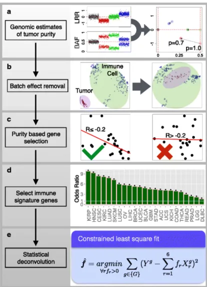
TIMERwas developed to study the interactions of tumor-infiltrating immune cells with the surrounding cancer cells [42]. In Figure 1.4 the deconvolution workflow is shown. First, several pre- processing steps are carried out, e.g., the sample purity is calculated. The surrogate for tumor purity is the fraction of aneuploid cells (a). Then, batch effects need to be removed (b). Next, genes which are negatively correlated with tumor purity are selected. Those, which have expression levels strongly affected by the purity of the tumor are tested for immune signature enrichment (c).

Next, the top 1% of the strongest expressed genes are removed, since they dominate the inference of results (d). Finally the deconvolution of a mixtureY is calculated by (e):

f = argmin

∀r:fr>0

X

g∈{G_Of}



Y^g− X

all cell typesr

f_rX_r^g



, (1.4)

whereY^g is the gene expression of geneg, withg∈G_Of. HereG_Of collects the genes which remain after the filtering steps. The expression of genegin cell type ris given by Xr^g andfr is the amount of cell type r in the mixture Y.

CIBERSORT A second state-of-the-art method is CIBERSORT [43]. Here, a linear support vector regression (SVR) algorithm with adaptive feature selection is used to devonvolute bulk mixtures. Figure 1.5 gives an overview of the deconvolution process.

CIBERSORT needs a matrix of gene expression profilesX and a bulk gene-expression profileY as an input. The cell fractionsC are defined through

Y =XC. (1.5)

CIBERSORT uses ν-support vector regression, which is an optimization method for binary classification problems. Here two classes are separated by a hyperplane with maximal margins. The

(23)

Figure 1.4: The five steps of TIMER for calculating the distribution of immune cells in a bulk sample. (a) calculation of the tumor purity and removing batch effects (b). Gene selection using tumor purity (c). Removing of the strongest expressed genes (d). Finally the cellular proportions are estimated by a con- strained linear regression problem (e).

Picture from [42]

(24)

Figure 1.5: Schematic representation of CIBERSORT. Transcriptome profiles of purified cells are used to construct the gene expression signature matrix X. With this, the transcriptome profile of a tumor bulk Y is deconvoluted by a ν-support vector regression algorithm. After significance thresholding, the relative cell-type fractions C are returned. Picture from [43].

Figure 1.6: Visualization ofν-vector regression for two different choices of ν.

The solid black line represents the regression line and the red points the support vectors. Picture from [43].

hyperplane boundaries are determined by a subset constituted by the input data. This subset supplements the vectors. Support vector regression fits a hyperplane with as many data points as possible within a distance . The points outside the environment of the regression line are the support vectors shown as red points in Figure 1.6. The algorithm minimizes a linear combination of two functions:

1. The loss function which measures the error associated with data fitting by a linear-insensitive loss function.

2. The penalty function that determines the complexity of the model. Here it is a L2-norm penalty.

The resulting cell-type proportions C are normalized to a sum of one.

(25)

Chapter 2

Methods

In this chapter the mathematical background of loss-function learning for digital tissue deconvolution is presented. Section 2.1 introduces the used notation. Section 2.2 gives the mathematical background of loss-function learning. In section 2.3, it is proved that the corresponding optimization problem is non-convex. Finally, a line search algorithm with adaptive step size is presented in section 2.4 and it gets shown that this algorithm is able to find the most informative genes for deconvolution in a simulation study, as seen in section 2.5.

2.1 Notations

LetX∈R^p×q be a matrix with cellular reference profilesX·,j in its columns, where the dot stands for all row indices. X_ij is the reference expression value of gene i in cells of type j, p the number of genes, andq the number of cell types inX, respectively. Further a matrix Y ∈R^p×n with bulk profiles ofncell mixturesY·,k in its columns and a matrix C∈R^q×n with the cellular compositions of the mixturesC·,k as columns is introduced.

2.2 Loss-Function Learning

Following the established linear DTD algorithms, the mixture Y·,k is approximated by a linear combination of reference profiles (the columns ofX) with C.,k as weights and the composition of thek-th mixture C·,k is estimated by minimizing

L_g(Y·,k−XC·,k), (2.1)

where

L_g =||diag(g)(Y_·,k−XC·,k)||²₂. (2.2) In contrast to standard DTD algorithms, which determinegby prior knowledge or separate statistical analysis,gis learned directly from data. To this end it is assumed that a training set of mixtures

(26)

Y·,k from a specific application context with known cellular proportions C·,k with sum one exists.

The entries of g are the gene weights that define the loss function. The aim of the here presented algorithm is to learng from the training data such that minimizingL_g(y−Xc) with respect to c yields accurate quantifications of cell populations for future samples with similar characteristics as those used for training.

The newly developed method has two nested objective functions: An outer function L(g) and an inner function L_g, which is here given by equation (2.2). L evaluates discrepancies between the estimated and the true cellular frequencies of cell types across samples by Pearson correlation:

L(g) =−

q

X

j=1

cor(Cj,·,Cˆj,·(g)) subject to gi ≥0 and ||g||₂ = 1, (2.3)

where the ˆCj,·(g) are the estimates of Cj,· given g. To evaluate L(g) it is necessary to calculate all Cˆj,·(g), which requires optimising L_g with respect to allC·,k. Note that if ˆg is a minimum of L, so isαgˆforα >0. The constraint ||g||₂ = 1 is thus needed to ensure unique solutions. Note that

cor(Cj,·, a_jCˆj,·) = cor(Cj,·,Cˆj,·), (2.4) where a_j is an arbitrary positive constant. This symmetry is important, since bulk and reference profiles must be normalized to a common mean across genes or to a common library size. A normalized reference profile X·,j of a cell type reflects the true RNA content ˜X·,j of these cells only up to an unknown factor: X·,j =α_jX˜·,j. Large cells with a lot of RNA have smaller α_j than smaller cells. The same is true for the bulk profilesY·,k, where the relationY·,k =βkY˜·,k holds. The deconvolution equation

Y˜_·,k = ˜XC˜_·,k+ (2.5)

yields estimates for ˜C_jk that reflect the number of cells of type j. However, ˜Y and ˜X are not observable in practice and consequently, ˜C is not accessible by DTD directly. So, one needs to work withX andY instead.

Note that C·,k = ˜C·,k/Pq

j=1C˜_jk. Consider now the hypothetical deconvolution formula with normalized Y but the unobservable true ˜X

Y·,k = ˜XC_·,k⁰ + . (2.6)

Here, it is assumedC_·,k⁰ =c C·,kfor allk, wherecis a positive constant. In other words it is assumes that if the library size ofY·,k is the same for all samples, roughly the same number of cells are needed to account for it. This assumption allows to replace ˜Y by Y.

The choice of the correlation in the definition of L(g) also allows to replace ˜X by X. If Eq.

(2.6) is written using X,

Y·,k=

q

X

j=1

1 αj

X·,jC_jk⁰ + (2.7)

(27)

is obtained Thus, the estimated cell frequencies are _α¹

jC_j,·⁰ = _α^c

jCj,·, and can be quite different from the training proportions Cj,· in absolute numbers. Nevertheless, they correlate with Cj,· and will thus generate small lossesL(g).

In summary, data normalization makes tissue deconvolution a non-standard deconvolution problem. The choice of correlation as loss function allows for estimation of cell frequencies independent of normalization factors.

The minimum ofL_g can be calculated analytically, yielding

C(g) = (Xˆ ^TΓX)⁻¹X^TΓY (2.8)

with Γ = diag(g). Inserting this term into L leaves a single optimization problem in g. L is minimized by a gradient-descent algorithm. Letµ_j and σ_j be the mean and standard deviation of Cj,·, respectively. For the gradient (for more detailed calculations see Appendix A)

∂L(g)

∂g_i =−

q

X

j=1 n

X

k=1

∂

cor(Cj,·,Cˆj,·)

∂Cˆjk

∂Cˆ_jk(g)

∂g_i

=

q

X

j=1 n

X

k=1

1 σ_jσˆ_j

cov(Cj,·,Cˆj,·) nˆσ_j²

Cˆ_jk−µˆ_j

− 1

n(C_jk−µ_j)

!∂Cˆjk(g)

∂g_i . (2.9)

is obtained. With equation 2.8 one gets for the partial distribution ^∂^C^ˆ_∂g^jk^(g)

i

∂Cˆ_jk

∂gi

= ∂

∂gi

(X^TΓX)⁻¹X^tΓY

jk

= −(X^TΓX)⁻¹ X^Tδ(i)X

(X^TΓX)⁻¹X^TΓY + (X^TΓX)⁻¹X^Tδ(i)Y

jk . Written as a matrix one gets

∂C(g)ˆ

∂gi

= (X^TΓX)⁻¹X^Tδ(i) 1−X(X^TΓX)⁻¹X^TΓ

Y , (2.10)

whereδ(i)∈R^p×p is defined as

δ(i)_jk =n 1 ifi=j=k,

0 else. (2.11)

The constraints ||g||₂ = 1 and g_i ≥ 0 were incorporated by normalizing g by its length and by restricting the search space togi ≥0.

(28)

Figure 2.1: Left region is convex. For every two points in X, the connection line is also in X. The right region is not convex.

One can find two points x and y where the line-segment joining these pointsxandy lies outside of the gray set X. Picture from [44].

x x+(1- )y)

y f(x)

f(

f(y) f(x)+(1- )f(y)

x+(1- )y

Figure 2.2: An example for a convex function. The connecting line for everyx, y∈X lies on or above the functionf. Picture from [45].

2.3 Loss-Function Learning Problem is not Convex - Counterex- ample Shown for Hessian with Negative Eigenvalues

Here, it is shown that the loss-function Equation 2.3 is non-convex.

Definition 2.3.1 X⊂Rⁿ is a convex set, when for every pair of points within the region, every point on the straight line segment that joins the pair of points is also within the region, thus

∀x, y∈X :∀λ∈[0,1] :x+λ(y−x)∈X. (2.12) Let X ⊂Rⁿ be convex. A function f :X →Ris called convex, if

∀x, y∈X :∀λ∈[0,1] :f(x+λ(y−x))≤f(x) +λ(f(y)−f(x)). (2.13) Figure 2.1 shows an example for a convex and a nonconvex region and Figure 2.2 shows a convex function.

Definition 2.3.2 A matrixA∈R^n×n is called symmetric, if

A^T =A. (2.14)

Definition 2.3.3 A symmetric matrixA is called positive semidefinite, when the corresponding quadratic form q_A is positive semidefinite, that means

qA(x)≥0 ∀x∈Rⁿ, x6= 0. (2.15)

(29)

The quadratic form is given by

qA(x) =x^TAx ∀x∈Rⁿ, x6= 0. (2.16) Definition 2.3.4 Let D ∈ R be a non-empty, open subset. Let k be a non-negative integer. The function f is said to be ofdifferentiability class C^k if the derivativesf, f⁰,. . ., f^(k) exist and are continuous.

Theorem 2.3.5 Taylor’s theorem with Peano remainder term Let f : [a, b] → R ∈ Cⁿ⁺¹, n∈N, x0 ∈(a, b). This implies the formula for the remainder term of Lagrange

f(x) =

n

X

k=0

f^(k)(x0)

k! (x−x0)^k+Rn(x;x0), (2.17) where Rn(x;x0) is given by

R_n(x;x₀) := f⁽ⁿ⁾(ξ)−f⁽ⁿ⁾(x0)

n! (x−x₀)ⁿ for a ξ∈[0,1]. (2.18) Furthermore it holds for the remainder term in then-th order that

Rn(x;x0) =o((x−x0)ⁿ) for x→x0. (2.19) proof: For proof see K¨onigsberger, Analysis 2 [46].

Theoin theorem 2.3.5 is little-o-notation by Landau. The notationf =o(g) orf ∈o(g) means thatf is growing slower than g.

Theorem 2.3.6 Criterion of convexity (see [46])

Let f :U →Rbe a C²-function on a convex and open set U. Then:

i) f is convex if and only if f⁰⁰(x)≥0 ∀x∈U. ii) f is strictly convex if f⁰⁰(x)>0 ∀x∈U.

proof: For proof see K¨onigsberger, Analysis 2 [46].

As the calculation ofU is not taking place inR, but inR^p, the theorem needs to be upgraded:

Theorem 2.3.7 For f ∈ C² and X⊂Rⁿ open, convex and nonempty holds:

f is convex on X if and only if ∀x∈X : ∇²f(x) is positive semidefinite.

proof: ⇒: Show first:

f ∈ C¹(Rⁿ), X ∈ Rⁿ is convex and not empty. Then:

f is convex in X ⇔ ∀x, y∈X:f(y)≥f(x) + (∇f(x))^T(y−x). (2.20)

(30)

First the direction “⇒” of equation (2.20) is proven. Let f be convex onX, then f(x+λ(y−x))≤f(x) +λ(f(y)−f(x)) ∀λ∈[0,1],∀x, y∈X.

⇒ Ψ(λ) :=f(x) +λ(f(y)−f(x))−f(x+λ(y−x))≥0. (2.21) As f ∈ C²(Rⁿ) it ensues that Ψ(λ) is continuously differentiable as composition of continuously differentiable functions and Ψ(0) = 0. So

Ψ⁰(λ) =f(y)−f(x)−(∇f(x+λ(y−x)))^T(y−x)

Ψ⁰(λ) =f(y)−f(x)−(∇f(x))^T(y−x). (2.22) Ψ(λ)≥0 and Ψ(0) = 0 implies Ψ⁰(0)≥0 because Ψ∈C²(Rⁿ). It follows with equation (2.22) for f(y) that

f(y)≥f(x) + (∇f(x))^T(y−x). (2.23) Second, direction “⇐” of equation (2.20) is proven. Let y be given by y = x+tc with x ∈ X, c∈Rⁿ andt >0 sufficiently small. SinceX is convex and not empty it follows that for sufficiently small talso y=x+tc∈X ∀c∈Rⁿ. With Equation (2.22) follows

0≤f(x+tc)−f(x)−t(∇f(x))^Tc. (2.24) With the Taylor formulas in theorem 2.3.5 and xTaylor = x +tc and x0,Taylor = x follows for f(y) =f(x+tc)

f(x+tc) =f(x) + (∇f(x))^T(x+tc−x) + 1

2!(x+tc−x)^T∇²(x+tc−x)² + (x+tc−x)^T∇²f(ξ)− ∇²f(x)

2! (x+tc−x)

| {z }

o(t²)

. (2.25)

With equation (2.25) it follows for equation (2.24) f(x+tc)−f(x)−t(∇f(x))^Tc=1

2t²c^T∇²f(x)c+o(t²)≥0 |: t² 2 c^T∇²f(x)c+2o(t²)

t² ≥0 (2.26)

Witht→0 + 0 one gets

t→0+0lim

c^T∇²f(x)c+2o(t²) t²

≥0. (2.27)

Therefore the Hessian is positive semidefinite.

Now the other direction of the theorem is shown.

(31)

⇐: Now the assumption is∀x∈X:∇²f(x) is positive semidefinite.

One has to show thatf is convex (see definition ).

Asf ∈ C² andX is open, convex and nonempty, there exists for everyx, y∈X aξ∈]0,1[ such that

f(y) =f(x) + (∇f(x))^T(y−x)−1

2(y−x)^T∇²f(x+ξ(y−x))(y−x) (2.28) holds. As∀x∈X it holds that∇²f(x) is positive semidefinite and sox^T∇²f(x)x≥0∀x∈X (see definition 2.3.3). It follows

1

2(y−x)^T∇²f(x+ξ(y−x))(y−x)≥0. (2.29) With equation (2.28) this yields

f(y)≥f(x) + (∇f(x))^T(y−x). (2.30) Let x := x+x+λ(y−x) with λ ∈]0,1[. x ∈X forx, y ∈ X since X is convex. Using equation (2.30) with (x, y) = (x, x) and with (x, y) = (x, y) yields

f(x)≥f(x) + (∇f(x))^T(x−x) | ·(1−λ) + f(y)≥f(x) + (∇f(x))^T(y−x) | ·λ

(1−λ)f(x) +λf(y)≥f(x+λ(y−x)) + 0 (2.31)

which is the definition of convergence (see 2.3.1).

To prove non-convexity, theorem 2.3.7 gets applied. It holdsg_i≥0 ∀ i∈1, . . . , p. Note that at least as manyg_ineed to be non-zero as cell types are included. Otherwise the corresponding system of equations remains under determined. Further the normalization||g||= 1 is to ensure uniqueness of the solution. Here this constraint is neglected, since it does not change the subsequent arguments.

G is part of a p−dimensional sphere and G is nonempty and convex. Furthermore, G is not open sinceg_i ≥0 ∀ i∈ 1. . . p. First the inner part ˚Gof the region G is considered. Figure 2.3 illustrates the region G for g ∈ R³ for 3,2 and 1 cell type, respectively. For q ≥ 1, ˚G is convex, nonempty and open. Furthermore, the covariance and the standard deviation areC^∞ and thus also C(g) isˆ C^∞, where it gets assumed that the standard deviation remains non-zero in general.

The Hessian of the outer loss-function L(g) is given by (for more detailed calculations see

(32)

Figure 2.3: For three genes x, y and z and three cell types the allowed regionG corresponds to the green area. For two cell types G corresponds to the green area and its border (blue), where the linesx=y= 0,z=y= 0, andx=z= 0 are excluded. Theorem 2.3.7 is only valid onG. Picture from [47].

Appendix A)

H_li(g) = ∂

∂g_l ∂L

∂g_i

=

q

X

j=1 n

X

k=1

∂

∂g_l

∂(−cor(C_j,·,Cˆj,·))

∂Cˆjk

·∂Cˆ_jk(g)

∂g_i

!

=

q

X

j=1 n

X

k=1











"

∂

∂Cˆ_jk

∂(−cor(C_j,·,Cˆj,·))

∂Cˆ_jk

!#

| {z }

A

∂Cˆ_jk(g)

∂gl

·∂Cˆ_jk(g)

∂gi

+ ∂(−cor(C_j,·,Cˆj,·))

∂Cˆ_jk · ∂

∂g_l

∂Cˆ_jk(g)

∂g_i

!

| {z } B











. (2.32)

(33)

For A and Bone gets A = 1

nσjσˆ_j³(ˆµ_j−ˆc_j,k) cov(Cj,·,Cˆj,·) nˆσ_j²

Cˆ_jk−µˆ_j

− 1

n(C_jk−µ_j)

!

+ 1

n²σjσˆ_j³

"

(C_jk−µ_j)( ˆC_jk−µˆ_j)− 2 ˆ

σ_j²cov(Cj,·,Cˆj,·)( ˆC_jk −µˆ_j)² +(n−1)cov(Cj,·,Cˆ_j,.)i

(2.33) and

B

= (X^TΓX)⁻¹X^T

δ(l)X(X^TΓX)⁻¹X^Tδ(i)(−1 +X(X^TΓX)⁻¹X^TΓ) +δ(i)X(X^TΓX)⁻¹

X^Tδ(l)X(X^TΓX)⁻¹X^TΓ−X^Tδ(l) Y

j,k. (2.34)

Non-convexity is shown by a counter example. Here, specific values for X, C, and Y are chosen, subject to the constraints

1. Xi,j ≥0 ∀i∈ {1, . . . , p} and ∀j∈ {1, . . . , q}, 2. C_j,k ≥0 ∀j ∈ {1, . . . , q}and ∀ k∈ {1, . . . , n}, 3. Y_i,k ≥0 ∀ i∈ {1, . . . , q}and ∀ k∈ {1, . . . , n}.

For the reference matrixX

X =







1 0 0 0 2 0 0 0 3 0 0 4







(2.35)

is chosen and for the distributions inC

C =



 2 1 4 6 3 2



. (2.36)

The bulk profilesY were chosen as

Y =





 1 5 2 6 3 7 4 8







. (2.37)

To prove non-convexity, it has to be shown that the Hessian matrix has negative Eigenvalues. For calculating the Hessian H the reference matrix X and the bulk profile Y are normalized to 100 counts in every column. The compositionC is normalized to 1 for each column.

(34)

The estimated bulk profiles ˆC are calculated with equation (2.8) by using g= (¹₄,¹₄,¹₄,¹₄).

Equation (2.32) yields the Hessian H,

H =







0 0 0 0

0 0 14.959681 6.333319 0 0 6.333319 −27.626320







. (2.38)

The Eigenvalues are 15.88160, 0, 0 and -28.54824.

One of four of the Eigenvalues is negative. Thus, function equation (2.3) is non-convex for X, C, and Y as given by equations (2.35), (2.36), and (2.37). With theorem 2.3.7 the Hessian of the regarded loss-function learning problem is not convex in ˚G and therefore not onG.

2.4 Algorithm for Loss-function Learning

Here, the used algorithm for loss-function learning is presented. This algorithm uses a coordinate descent in condition with line search. The update step is

g_{step s}=gstarting point+step size

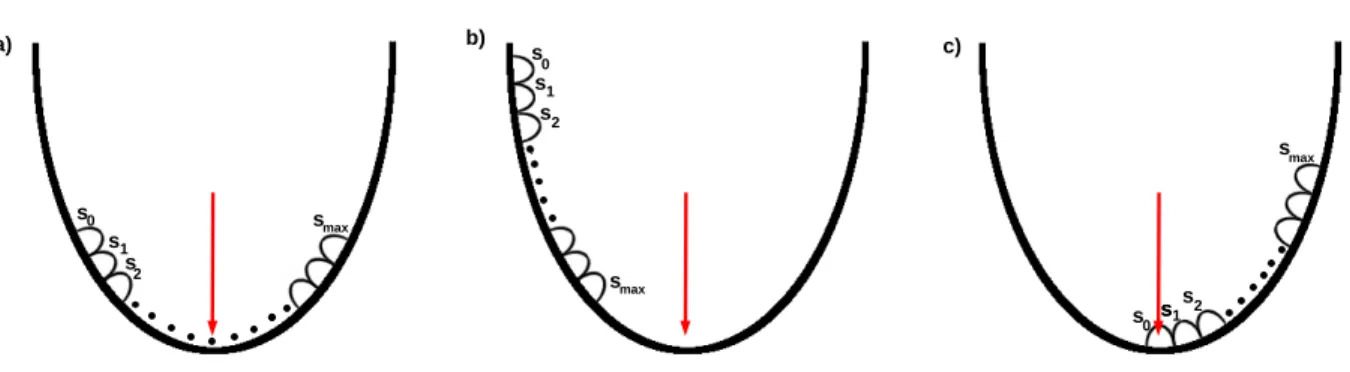
s_max ·s· ∇L fors∈ {0,1, . . . , s_max}, (2.39) where∇L is the gradient of the loss function. Step size is the step length in the direction∇L and smax is the maximum number of points that are evaluated along the gradient. Further negative entries ingstep sare set to zero such that the constraintgi≥0 holds. For every steps∈ {0,1, . . . , smax} one calculates the corresponding g_s and the value of the loss-function L. There are three possible cases where the position of the optimalsopt, which corresponds to the minimum in the loss-function L, is localized. All cases are exemplified in Figure 2.4:

1. The loss-function L takes its minimum for s_opt ∈ {1,2, . . . , s_max−1}. In this case, it gets updated and the next iteration starts:

g_{new start} =g_s_opt (2.40)

2. L takes its minimum forsopt =smax. Here, the maximum in the direction of the gradient is not yet reached. The search continues in the direction of the calculated gradient and gets not updated in the next iteration. The new starting point of the gene weight is

g_{new start} =g_s_max (2.41)

and the step size in the next iteration is doubled.

3. L takes its minimum for s_opt = 0. So the starting point for g is very near to the maximum in the direction of gradient. To find a better solution, the same starting vectorg is used and the step size is divided by 10. Here, an update of the gradient is not necessary.

(35)

s a)

ss

s_max

1 0

2

v

b) s s

s

s_max

1 0

2

s c)

s_max

0 1

ss2

s

Figure 2.4: The three cases of minimum positions are shown here. The red arrow points to the minimum of the loss-function. In figure (a) the minimum is reached within the number of steps.

In figure (b) the minimum is not reached after the maximal step number, therefore the step size is increased. In figure (c) the starting steps0 is too near to the minimum of the loss function, which makes it necessary to reduce the step size.

As starting step size the number of steps is chosen in order to minimize the number of initial parameters. Then, in every iteration either the gradient or the step size is updated. When a minimum of the loss-functionLis reached insopt ∈ {1,2, . . . , smax−1}a new gradient is calculated (Figure 2.4 a). The step size is updated when the minimum is not yet reached or if it is reached in the first step, receptively (Figure 2.4 b an c). The number of steps is given by the user. For initializationg= (1, ...,1) gets used.

2.5 Simulation Study on Artificial Data

In this section it gets shown that loss-function learning reliably identifies cell markers for DTD.

A reference matrix X1 consisting of four reference profiles (columns) and six genes (rows) gets defined as

X₁=







8 4 0 0 3 6 0 0 0 0 7 4 0 0 1 5 5 2 9 9 6 2 9 7







, (2.42)

and normalized column-wise to a value of 100.

The cellular compositions of the artificial bulk profiles were simulated by randomly drawing values between zero and one for each cell type and then normalized to the sum of 1. By multiplying the reference matrixX₁with the cellular compositions inC, bulk profilesY are obtained. 50 artificial bulk profiles for testing are simulated and normalized like the reference profiles. In order to proof the autonomy of the learned models from the training data 100 different cellular compositions C

(36)

are simulated to give 100 different artificial training mixtures. Every training mixture consists of 100 artificial bulk profiles.

In the presented loss-function learning scenario, column 3 and 4 of X get ignored and only the first two get used for loss-function learning.

The gene weight of q1

6 is assumed for every gene in the beginning. This yielded a mean correlation of 0.673±0.039 for the training sets and of 0.673 in the test set for the two cell types.

The estimated gene weights are given in Table 2.1.

std. model 0.637 ±0.039

gene 1 0.748 ±0.005

gene 2 0.252 ±0.005

gene 3 0 ±0

gene 4 0 ±0

gene 5 0 ±0

gene 6 0 ±0

loss-fct. learned model 1 ±0

Table 2.1: Mean value and standard deviation for 100 complete optimization runs applied to the ideal loss-function learning problem. Each was optimized for 100 different randomly chosen cellular compositions. Only for the two genes which carry information the algorithm calculated a gene weight greater than zero. The corresponding average correlation for the two considered cell types was close to 1 on simulated test data.

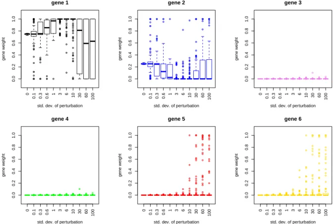
The algorithm obtained non-vanishing weights for gene 1 and 2, while the other gene weights were equal to zero. Thus, the algorithm correctly selected those genes which had a vanishing contribution in cell types 3 and 4. The results of the gene vectors after loss function learning were manipulated for all genes, to check their influence on the overall deconvolution result. For this manipulation a random value between zero and one for the gene of interest were taken and then the manipulated vector of gene weightsg were renormalized again to one. With these new gene vectors the artificial bulk of the test set was deconvoluted. Results can be seen in table 2.2.

manipulation in result of loss-fct. learned model

no manipulation 1 ±0

gene 1 1 ±0

gene 2 1 ±0

gene 3 1 ±0

gene 4 1 ±0

gene 5 0.870± 0.098

gene 6 0.840± 0.106

(37)

Table 2.2: Mean value and standard deviation for 100 complete optimization runs applied to of the ideal loss-function learning problem before and after gene manipulation. The results are shown on the test set.

Manipulation in gene one and two had no influence on the deconvolution results. The loss-function learning problem in this case is purely analytically solvable. The gene weight corresponds to a multiplication of the first two rows of Y = XCˆ with a constant value. This has no influence on the solution ˆC. Gene three and four did not contribute to the deconvolution and consequently the average correlation over the considered cell types did not change. Here the values in the reference matrix are zero and thus, according to equation (2.8), a non-zero value in g, i.e. in Γ, had no influence on the resulting cell-type distribution ˆC(g). For the genes five and six a manipulation led to a decreased value for the overall correlation. For these genes the reference matrix has non- vanishing entries for all four cell types. Here, the deconvolution of cell type 1 and 2 is confounded by the amount of cells of type 3 and 4 and consequently the performance gets lower in accuracy.

Next, the reference matrix X was changed slightly and the first two cell types were considered for deconvolution, as previously. The new reference matrix becomes

X2=







8 4 5 0 3 6 0 0 0 0 7 4 0 0 1 5 5 2 9 9 6 2 9 7







. (2.43)

The remaining simulation study was designed as previously (100 training sets with 100 artificial bulk profiles each and 50 artificial bulk profiles as test set). The results are shown in Table 2.3:

std. model (training set) 0.655±0.041

gene 1 0.751±0.005

gene 2 0.248±0.005

gene 3 0 ±0

gene 4 0 ±0

gene 5 0±0.001

gene 6 0 ±0

loss-fct. learned model (test set) 0.906 ±0

Table 2.3: Mean value and standard deviation for 100 complete optimization runs applied to the ideal loss-function learning problem. Results forX₂. The results are shown for the test set.

Although the gene weights were similar to the first simulation study, the performance analytically from a correlation of 1 to 0.906. Note that the deconvolution problem is no longer perfectly solvable due to confounding contribution of cell types 3 and 4. The gene weights were manipulated as in the previous simulation study and yielded the results shown in Table 2.4.

(38)

manipulation in result of loss-fct. learned model

no manipulation 0.906 ±0

gene 1 0.906± 0.001

gene 2 0.906 ±0

gene 3 0.906 ±0

gene 4 0.906 ±0

gene 5 0.781± 0.080

gene 6 0.784± 0.068

Table 2.4: Mean value and standard deviation for 100 complete optimization runs applied to the ideal loss-function learning problem before and after gene manipulation. The shown results correspond to reference matrixX₂ and are again evaluated on test data.

Manipulating the genes two to four had no influence on the results as discussed previously. Also manipulation of gene one had no influence. As the gene weights vectors were heavy on the first two genes and the others only showed vanishing entries, equation (2.8) led to a simplified equation system consisting of two equations for two variables. This reduced mathematical expression again is perfectly solvable. A change in the gene weight vector of gene one corresponds to a multiplication of the corresponding equationgY =gXc, with a constant factor and has therefore no influence on the results. The last two genes had entries in all cell types and thus a change in the gene weights led to lower correlations than in the first simulation study which was shown above.

As third example the reference matrix X₃ is considered,

X3 =







0 0 8 4 0 0 3 6 7 4 5 7 1 5 3 4 9 9 5 2 9 7 6 2







. (2.44)

Now, there are zeros in the first two genes of the two investigated cell types. The realization of the experiment was the same as in X₁ and X₂. The results for the gene weights and their standard deviation are itemized in table 2.5.

std. model (training set) 0.954 ±0.050

gene 1 0.013 ±0.018

gene 2 0.013 ±0.018

gene 3 0.025 ±0.032

gene 4 0.031 ±0.042

gene 5 0.897 ±0.136

gene 6 0.020 ±0.028

loss-fct. learned model (test set) 0.971 ±0.002