Construction Sequences and Certifying 3-Connectivity

Construction Sequences and Certifying 3-Connectivity

Journal Version ^∗

Jens M. Schmidt

Institute of Computer Science Freie Universität Berlin, Germany

Abstract

Tutte proved that every 3-vertex-connected graph G on more than 4 vertices has a contractible edge. Barnette and Grünbaum proved the exis- tence of a removable edge in the same setting. We show that the sequence of contractions and the sequence of removals from G to K

can be com- puted in O(|V |

) time by extending Barnette’s and Grünbaum’s theorem.

As an application, we derive a certificate for the 3-vertex-connectivity of graphs that can be easily computed and verified.

1 Introduction

For a given set O of operations and a given set B of base graphs, a construction sequence of a graph G is a sequence of operations in O that constructs G when being applied to a base graph in B. For 3-vertex-connected (we say 3-connected) graphs G, we focus on construction sequences with B = {K

} and for which O consists either of inverse contractions (Tutte’s construction sequence) or in- verse removals (Barnette’s and Grünbaum’s construction sequence). These two construction sequences are the inverse of the sequence of contractions and the sequence of removals, respectively. We will define contractions, removals and their inverse operations in Section 2.

Inductively defined constructions of graph classes are important, because the set of operations used in the constructions can often be exploited to prove properties on these graph classes. For 3-connected graphs, the existence the- orems on contractible and removable edges yield such inductively defined con- structions. Although these existence theorems are used frequently in graph theory [12, 13, 16], we are not aware of any computational results to find the se- quence of contractions or removals, except for sequences where contractions and removals are allowed to intermix [1]. Moreover, efficient algorithms are unlikely to be derived from the existence proofs as they, e. g., in the case of Barnette and Grünbaum, depend heavily on adding longest paths, which are NP-hard

∗

This research was supported by the Deutsche Forschungsgemeinschaft within the research

training group “Methods for Discrete Structures” (GRK 1408) and is an extended version

of [11].

to find. The main contribution of this paper is a structural result about the existence of Barnette’s and Grünbaum’s construction sequence and, based on that result, a simple algorithm to compute such a sequence in time O(|V |

). In addition, we show that Barnette’s and Grünbaum’s construction sequence can be transformed in linear time to the sequence of contractions, obtaining a close connection between these two sequences and a simple quadratic time algorithm for computing Tutte’s construction sequence. Both algorithms do not rely on the 3-connectivity test of Hopcroft and Tarjan [6], which runs in linear time but is rather involved.

The concept of certifying algorithms, which give a small and easy-to-verify certificate of correctness along with their output, was initiated by Blum and Kannan [3] and developed further by McConnell et al. [8]. While being impor- tant for program verification, certifying algorithms often provide new insights into a problem, which can lead to new techniques. For that reason they are a major goal for problems on which the known fast solutions are complicated and difficult to implement. Testing a graph on 3-connectivity is such a problem.

Yet, surprisingly little work has been devoted to certify 3-connectivity, although a sophisticated linear-time recognition algorithm (not giving an easy-to-verify certificate) is known for over 35 years [6, 17, 18]. In fact, we are aware of only one certifying algorithm (in the sense of McConnell et al.) for that problem, which runs in quadratic time, but is quite involved [1]. Using construction sequences, we give a simple alternative solution with running time O(|V |

) that performs essentially DFS-traversals and show that the used certificate is easy-to-verify in time O(|E|).

We first recapitulate well-known results on the existence of construction se- quences in Sections 2.1 and 2.2 and point out how the sequence of contraction can be obtained from Barnette’s and Grünbaum’s sequence in linear time. Sec- tions 2.3 and 3 cover the main idea for the existence result that we use for computing Barnette’s and Grünbaum’s construction sequence. The end of Sec- tion 3 deals with the representation of construction sequences. Section 4 shows how to use construction sequences for a certifying 3-connectivity test.

2 Construction Sequences

Let G = (V, E) be a finite graph with n := |V |, m := |E|, V (G) = V and E(G) = E. A graph is connected if there is a path between any two vertices and disconnected otherwise. For k ≥ 1, a graph is k-vertex-connected if n > k and deleting every k −1 vertices leaves a connected graph. We will write k-connected throughout the paper when referring to k-vertex-connectivity. A vertex (resp.

a pair of vertices) that leaves a disconnected graph upon deletion is called a cut vertex (resp. a separation pair). Note that k-connectivity does not depend on parallel edges or self-loops. From now on, we assume for simplicity that our input graph G = (V, E) is simple, although all results can be extended to multigraphs. A path leading from vertex v to vertex w is denoted by v → w.

For a vertex v in a graph, let N(v) = {w | vw ∈ E} denote its set of neighbors and deg(v) its degree. For a graph G, let δ(G) be the minimum degree of its vertices.

A subdivision of a graph G is a graph that replaces each edge in E(G) by

a path of length at least one. Conversely, we want a function that returns the

original graph without subdivided edges. If deg(v) = 2 for a vertex v in a graph G, let smooth

(G) be the graph obtained from G by deleting v followed by adding an edge between its neighbors; we say v is smoothed. Otherwise, let smooth

(G) = G. Let smooth(G) be the graph obtained by smoothing every vertex in G. For an edge e ∈ E, let G \ e denote the graph obtained from G by deleting e. Let K

be the complete graph on n vertices.

The following are well-known corollaries of Menger’s theorem [9].

Lemma 1. (Fan Lemma) Let v be a vertex in a graph G that is k-connected with k ≥ 1 and let A be a set of at least k vertices in G with v / ∈ A. There are k internally vertex-disjoint paths P

, . . . , P

from v to distinct vertices a

, . . . , a

∈ A such that for each of these paths V (P

) ∩ A = a

.

Lemma 2. (Expansion Lemma [19]) Let G be a k-connected graph. The graph obtained by adding a new vertex v joined to at least k vertices in G is still k-connected.

2.1 Tutte’s Characterization and its Inverse

Although G is simple, contractions cannot always avoid parallel edges in inter- mediate graphs. E. g., consider a cycle with an additional vertex connected to all cycle vertices by an edge. This is a wheel graph, and the edges adjacent to the non-cycle vertex are called spokes. The contraction of any edge that is not a spoke in a wheel graph will create a parallel edge. That is why we define contractions to preserve graphs to be simple. Contracting an edge e = xy in a graph deletes e, merges vertices x and y, and replaces every set of parallel edges by a single edge. An edge e is called contractible if contracting e results in a 3-connected graph.

A vertex splitting takes a vertex v of a 3-connected graph, replaces v by two vertices x and y with an edge between them and replaces every former edge uv that was incident to v with either the edge ux, uy or both such that |N (x)| ≥ 3 and |N (y)| ≥ 3 in the new graph. Vertex splitting as defined here is therefore the exact inverse of contracting a contractible edge that has end vertices of degree ≥ 3.

Theorem 3. (Corollary of Tutte [15]) The following statements are equivalent:

A simple graph G is 3-connected

⇔ There exists a sequence of contractions from G to K

on contractible (1) edges e = xy with |N(x)| ≥ 3 and |N(y)| ≥ 3

⇔ There exists a construction sequence from K

to G using vertex (2) splittings

We describe next a straightforward O(n

) algorithm to compute (1) for a graph G on more than 4 vertices. First, we decrease the number of edges to O(n) in G by applying the following algorithm due to Nagamochi and Ibaraki.

Theorem 4 (Nagamochi, Ibaraki [10]). Let G be a connected graph and k ∈ N . There is an O(m) time algorithm computing a spanning subgraph of G that has at most k(n− 1) edges and is k-connected (resp. k-edge-connected) if and only if G is k-connected (resp. k-edge-connected). Moreover, if G is k-connected (resp.

k-edge-connected), the spanning subgraph contains a vertex of degree k.

This algorithm preserves the 3-connectivity or respectively, that G is not 3- connected. Moreover, if G is 3-connected, the resulting graph contains a vertex of degree 3 and by a result of Halin [5], every vertex of degree 3 is incident to a contractible edge e. We get e by subsequently contracting each of the three incident edges and testing the resulting graph with the algorithm of Hopcroft and Tarjan [6] on 3-connectivity. Iteration of both subroutines gives us the whole contraction sequence in O(n

) time. However, the Hopcroft-Tarjan test is difficult to implement and we will give a much simpler algorithm that is capable of computing both characterizations later. In both approaches, we use the algorithm of Theorem 4 to preprocess the input graph G in advance.

2.2 Barnette’s and Grünbaum’s Characterization and its Inverse

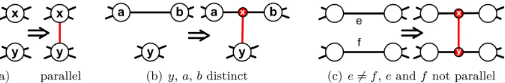
The Barnette and Grünbaum operations (BG-operations) consist of the follow- ing operations on a 3-connected graph (see Figures 1(a)-1(c)).

(a) add an edge xy (possibly a parallel edge)

(b) subdivide an edge ab by vertex x and add the edge xy for y / ∈ {a, b}

(c) subdivide two distinct, non-parallel edges by vertices x and y, respectively, and add the edge xy

In all three cases, let xy be the edge that was added by the BG-operation.

(a) parallel edges allowed

(b) y, a, b distinct (c) e 6= f, e and f not parallel

Figure 1: The three operations of Barnette and Grünbaum.

Theorem 5. (Barnette and Grünbaum [2], Tutte [16]) A graph G is 3-connected if and only if G can be constructed from K

using BG-operations.

Theorem 5 was proven in this notation by Barnette and Grünbaum [2], but also described in results about nodal connectivity by Tutte [16, Theorems 12.64 and 12.65]. If not stated otherwise, every construction sequence uses only BG- operations. Let a BG-operation be basic, if it does not create parallel edges and let a construction sequence be basic, if it only uses basic BG-operations.

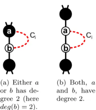
Like in Theorem 3, we want the inverse of a BG-operation. Let removing the edge e = xy of a graph be the operation of deleting e followed by smoothing x and y. An edge e = xy in G is called removable, if removing e yields a 3-connected graph. We show that removing a removable edge e = xy with

|N (x)| ≥ 3, |N(y)| ≥ 3 and |N(x) ∪ N (y)| ≥ 5 is exactly the inverse of a

BG-operation.

(a) The vertices x and y are neigh- bored.

(b) The vertices x and y are both neighbored and of degree 2.

(c) Case in which

|N(x) ∪ N (y)| < 5.

Figure 2: Cases that would fail when undoing a removal.

Theorem 6. The following statements are equivalent:

A simple graph G is 3-connected (3)

⇔ There exists a sequence of removals from G to K

on removable (4) edges e = xy with |N (x)| ≥ 3, |N(y)| ≥ 3 and |N (x) ∪ N (y)| ≥ 5

⇔ There exists a construction sequence from K

to G using (5) BG-operations

⇔ There exists a basic construction sequence from K

to G using (6) BG-operations

Proof. Theorem 5 establishes (3) ⇔ (5). Moreover, the proof of Theorem 5 in [2]

implicitly shows that on simple graphs basic operations suffice. Thus, only the equivalence for (4) remains. We first prove (6) ⇒ (4) and then (4) ⇒ (5).

BG-operations operate by definition on 3-connected graphs, this holds in particular for the ones in sequence (6). Let G

be the graph obtained by a basic BG-operation in (6) that adds the edge e = xy. The operation can clearly be undone by removing e in G

. Since BG-operations preserve 3-connectivity with Theorem 5, |N (x)| ≥ 3 and |N(y)| ≥ 3 hold in G

.

It remains to show that |N (x) ∪ N(y)| ≥ 5 in G

. If |N(x)| ≥ 4 or |N(y)| ≥ 4, |N (x) ∪ N(y)| ≥ 5 follows, since x and y are neighbors and no self-loops exist. Thus, let |N (x)| = |N(y)| = 3. Having N (x) \ {y} 6= N(y) \ {x} yields

|N (x) ∪ N (y)| ≥ 5 as well, so let N (x) \ {y} and N (y) \ {x} contain the same two vertices a and b. If |V (G

)| > 4, a or b must be adjacent to a vertex c that is neither adjacent to x nor y. But then {a, b} is a separation pair, contradicting the 3-connectivity of G

. On the other hand, |V (G

)| = 4 is only possible when operation (a) was performed as BG-operation, since operations (b) and (c) create new vertices. This gives a contradiction, as (a) is not a basic operation on K

. We prove (4) ⇒ (5). Let G

be the graph containing a removable edge e = xy that is removed in (4). Note that G

can have parallel edges due to previous removals but no self-loops. The removal can be undone by one of the three BG-operations. On smoothing of e, we count how many end vertices are deleted. This is either 0, 1, or 2. If no end vertex is deleted, removing e just deletes e which is inverted by operation (a). If exactly one end vertex, say x ∈ V (G

), is deleted, let f be the edge in which x was smoothed. Then (b) can be applied, because y / ∈ f (see Figure 2(a)) since otherwise x would have had only 2 neighbors in G

, contradicting the assumption |N (x)| ≥ 3.

If both end vertices, x and y, are deleted, let f

and f

be the edges in which x and y were smoothed, respectively. Operation (c) can only be applied if f

and f

are neither identical nor parallel. But f

= f

would again contradict

|N (x)| ≥ 3 in G

(see Figure 2(b)), and f

being parallel to f

would contradict

|N (x) ∪N (y)| ≥ 5 in G (see Figure 2(c)), since in that case N(x)∪ N(y) consists only of x, y and the two vertices f

∩ f

.

We show that Barnette’s and Grünbaum’s characterization is algorithmically at least as powerful as Tutte’s by giving a simple linear time transformation.

Lemma 7 allows us to focus on computing BG-operations only.

Lemma 7. Every construction sequence using BG-operations can be trans- formed in linear time to the sequence (1) of contractions.

Proof. We transform every BG-operation in reverse order of the construction sequence to 0, 1 or 2 contractions each. Operation (a) yields no contraction while operation (b) yields the contraction of exactly one part of the subdivided edge (either xa or xb in Figure 1). For an operation (c), let e = ab and f = vw be the edges that are subdivided with x and y. Both edges share at most one vertex; w. l. o. g. let a = v be that vertex if it exists. We contraction the edges xb and yw in arbitrary order. In all cases, contractions inverse BG-operations except for the added edge xy, which is left over. But additional edges do not harm the 3-connectivity of the graph nor subsequent contractions. Thus, we have found a contraction sequence to K

unless the first contraction in the case of an operation (c) yields a graph H that is not 3-connected. Let H

be the 3-connected graph after the second contraction of the same operation (c).

Then H can be obtained from H

by applying operation (b) and therefore is 3-connected.

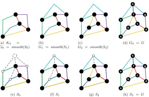
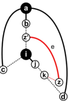
2.3 Identifying Intermediate Graphs with Subdivisions in G

Let K

= G

, G

, . . . , G

= G be the 3-connected graphs obtained in a construc- tion sequence Q to a simple 3-connected graph G using the basic BG-operations C

, . . . , C

. We can reverse Q by starting with G and removing the added edges of BG-operations in reverse order. Suppose we would delete the added edge of every C

instead of removing it and treat emerging paths containing interior vertices of degree 2 as (topological) edges in G

(see Figure 3). Then iteratively paths are deleted instead of edges being removed and we obtain the sequence of subdivisions G = S

, . . . , S

in G with S

being a K

-subdivision.

This leads to the following proposition.

Proposition 8. Let Q be a construction sequence from a graph G

to G using BG-operations. Then G contains a subdivision of G

that is specified by Q.

In particular, Proposition 8 yields with Theorem 5 that every 3-connected graph contains a subdivision of K

(Theorem of J. Isbell [2]). Each S

is a sub- division of G

. Conversely, G

= smooth(S

) for all 0 ≤ i ≤ z, since smoothing a graph is precisely the inverse operation of subdividing a graph without vertices of degree two. The vertices x in S

with deg(x) ≥ 3 are called real vertices, be- cause they correspond to vertices in G

. Real vertices have at least 3 neighbors in G

, because G

is 3-connected.

Note that in non-basic construction sequences G

can have parallel edges,

although S

is always simple.

(a) K

= G

= smooth(S

)

(b)

G

= smooth(S

) (c)

G

= smooth(S

)

(d) G

= G

(e) S

(f) S

(g) S

(h) S

= G

Figure 3: The graphs G

, . . . , G

and S

, . . . , S

of a construction sequence of G.

On graphs S

, the dashed edges and vertices are in G but not in S

and vertices depicted in black are real vertices. For example, the path C

= e → h → g is a BG-path for S

, yielding S

. The links of S

are the paths C

, a → b → c and the single edges ae, ef , f c, cd, da, f g, gd.

Definition 9. Let the links of each S

be the unique paths in S

with only their end vertices being real. Let two links be parallel if they share the same end vertices. Then a BG-path for S

is a path P = x → y in G with the following properties:

1. S

∩ P = {x, y}

2. If a link of S

contains x and y, the end vertices of that link are x and y.

3. If x and y are inner vertices of links L

and L

of S

, respectively, L

and L

are not parallel.

The links of S

partition E(S

) because S

is 2-connected, has therefore minimum degree two and is not a cycle. It is easy to see that every BG-path for S

corresponds to a BG-operation on G

and vice versa. We will exploit this duality in the next section.

In general, construction sequences are not bound to start with K

. Titov and Kelmans [14, 7] extended Theorem 5 by proving the existence of a construction sequence even when starting with an arbitrary 3-connected graph G

instead of K

, as long as a subdivision of G

is contained in G. This is a generaliza- tion of Theorem 5, since every 3-connected graph contains a K

-subdivision by Proposition 8.

Theorem 10. [7, 14] Let G

be a 3-connected graph. A simple graph G is

3-connected and contains a subdivision of G

if and only if G can be constructed

from G

using basic BG-operations.

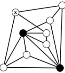
Figure 4: Every possible BG-operation adds a parallel edge to the black sub- graph.

3 Prescribing Subdivisions

If G is 3-connected, the 3-connected base graph G

of the construction sequences of Theorem 5 and 10 corresponds to a subdivision H ⊂ G of G

by Proposition 8.

The proofs of Theorems 5 and 10 show only for a very special subdivision H in G that a construction sequence from H to G using BG-paths exists. In fact, the G

-subdivision containing the maximum number of edges in G is chosen for both theorems. The construction sequence is then obtained by adding longest BG- paths. Unfortunately, computing these depends heavily on solving the longest paths problem, which is known to be NP-hard even for 3-connected graphs [4].

Suppose we choose some subdivision H of G

in advance; we say that H is prescribed. Is it possible to strengthen Theorems 5 and 10 to start a construction sequence using BG-paths with H? Such a result would provide an efficient computational approach to construction sequences, since it allows us to search the neighborhood of H in G for BG-paths, yielding a new prescribed subdivision of a 3-connected graph.

However, when restricted to basic operations it is not possible to prescribe H , as the minimal counterexample in Figure 4 shows: Consider the graph G consisting of H := K

depicted in black with an additional vertex x connected to three vertices of H. Then every BG-path for H will create a parallel link, which is a path of length two having x as its middle vertex, although G is simple. But what if we drop the condition that construction sequences have to be basic? The following theorem shows that at this expense we can indeed start a construction sequence from any prescribed subdivision.

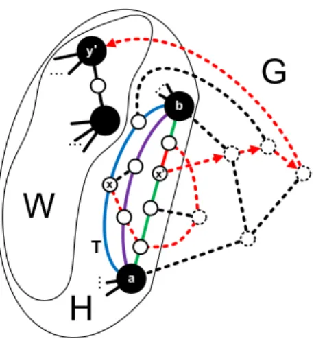
Theorem 11. Let G be a 3-connected graph and H ⊂ G with H being a subdi- vision of a 3-connected graph. There is a BG-path for H in G. Moreover, for every link L of H of length at least 2 there is a parallel link (maybe L itself) that contains an inner vertex on which a BG-path for H starts.

Proof. We distinguish two cases.

• H 6= smooth(H ).

Then links of length at least 2 exist in H and we pick an arbitrary one of them, say T = a → b. Let x be an inner vertex of T and let I be the union of inner vertices of all parallel links of T. We show that there is a vertex in I on which a BG-path for H starts. By the 3-connectivity of G, the graph G\{a, b} is connected. Since H contains at least four vertices, there exists a path P = x → y in G \ {a, b} with y ∈ V (H ) \ I (see Figure 5).

The path P has the Property 9.2. Let x

be the last vertex in P that

is contained in I and let y

be the first vertex in P that is contained in

V (H ) \ I. Then the subpath x

→ y

of P has Properties 9.1–9.3 and is a

BG-path for H.

Figure 5: The case H 6= smooth(H ). Dashed edges are in E(G) \ E(H ), arrows depict the BG-path x

→ y

.

• H = smooth(H ).

Then H consists only of real vertices and since H 6= G, there is a vertex in V (G) \ V (H ) or an edge in E(G) \ E(H ). At first, assume that there is a vertex x ∈ V (G) \ V (H). Then, by the 2-connectivity of G and Fan Lemma 1 we can find a path P = y

→ x → y

with no other vertices in H than y

and y

. For P the Properties 9.1-9.3 hold, because every link in H is an edge. Now suppose that V (G) = V (H ) and let e be an edge in E(G) \ E(H ). Then e must be a BG-path for H , since both end vertices are real.

In Theorem 11, non-basic operations can only occur in the case H = smooth(H ) when a path through a vertex of V (G) \ V (H ) is chosen. Although we cannot avoid that, it is possible to obtain a basic construction by augmenting the BG- operations with a fourth operation (d), which can be seen as combination of operations (a) and (b):

(d) connect a new vertex to three distinct vertices

Operation (d) preserves 3-connectivity with Lemma 2 and is basic, because each new edge ends on the new vertex. Whenever we encounter a vertex in V (G) \ V (H) in Theorem 11, we know by Fan Lemma 1 and the 3-connectivity of G that there are three internally vertex-disjoint paths to real vertices in H with all inner vertices being in V (G) \ V (H). Adding these paths to H is called an expand operation and corresponds to operation (d) in the smoothed graph.

This gives the following result.

Theorem 12. Let G be a simple graph and let H be a subdivision of a 3-

Figure 6: A 3-connected graph having a vertex x of degree 3 with no incident edge being removable. Removing each incident edge of x results in the black separation pair.

connected graph. Then

G is 3-connected and H ⊆ G

⇔ δ(G) ≥ 3 and there exists a construction sequence from H to G (7) using BG-paths

⇔ δ(G) ≥ 3 and there exists a basic construction sequence from H to G (8) using BG-paths and the expand operation

Proof. Let G be 3-connected and H ⊆ G. Then δ(G) ≥ 3 holds and if H = G, the desired construction sequences are empty and exist. If H ⊂ G, we can apply Theorem 11 iteratively with or without the additional expand operation and the construction sequences exist as well. For the sufficiency part, both construction sequences imply H ⊆ G, since only paths are added to construct G.

Additionally, G must be 3-connected, as adding BG-paths to each S

preserves S

to be a subdivision of a 3-connected graph with Theorem 5, and δ(G) ≥ 3 ensures that the last subdivision G of a 3-connected graph is 3-connected itself.

A straightforward algorithm to compute Barnette’s and Grünbaum’s con- struction sequence of a 3-connected graph is to search iteratively for removable edges. But in contrast to the algorithm in Section 2.1 that computes con- tractible edges, this approach only leads to an O(n

) algorithm. The reason for the additional factor of n is that not all vertices with degree 3 must have an incident removable edge (see Figure 6 for a counterexample on 9 vertices) and we have to try every edge in the worst case. Computing BG-paths instead of BG-operations allows us to obtain better running times. For this aim, we need to represent construction sequences.

An obvious representation of a construction sequence Q would be to store the graph G

= smooth(H) and in addition every BG-operation, which gives the sequence G

, . . . , G

= G. Unfortunately, the graphs G

are not necessarily subgraphs of G

, so we have to take care of relabeled edges when specifying each operation.

Whenever an edge e is subdivided as part of an operation (b) or (c), we specify it by its index in G

followed by assigning new indices to the new degree- two vertex and one of the two new separated edge parts in G

. The other edge part keeps the index of e.

Similarly, on operations (a) and (b), real end vertices of the added edge

are specified by their indices in G

. We assign a new index to the added edge

in G

, too. Finally, we have to impose the constraint that G

is not just isomorphic but identical to G, meaning that vertices and edges of G

and G are labeled by exactly the same indices, since otherwise we would have to solve the graph isomorphism problem to check that Q really constructs G.

On the other hand, the identification of G

with a subdivision S

in G allows us to represent Q without indexing issues: We just store S

⊂ G and the BG- paths C

, . . . , C

. Hence, we can represent each construction sequence Q of G in the following two ways.

• Edge representation: Represent Q by G

and a sequence of BG-operations, along with specifying new and old indices for each operation, such that G

and G are labeled the same.

• Path representation: Represent Q by S

and BG-paths C

, . . . , C

. Both representations refer to the same sequence of graphs G

, . . . , G

and are linear in the graph size. Assuming the uniform cost model, this size is Θ(m), as the uniform cost model is independent on the size of the numbers processed;

in particular, the space amount of each index is 1 instead of O(log n). The next lemma states that it does not matter which of the two representations we compute.

Lemma 13. The edge and path representations of a construction sequence Q can be transformed into each other in O(m) time. Moreover, the representation computed is a unique representation of Q.

Proof. Let G

and a sequence of BG-operations along with their specified indices on edges and vertices be given. If an operation O

subdivides an edge e

, we define β(e

, O

) to be the edge that gets a new index. Let e be the added edge of an operation in Q. Exploiting the duality of BG-paths and BG-operations, the edge e corresponds to a BG-path C, which will be subdivided by inserting

|C| − 1 vertices in the construction sequence. To compute the BG-path C from e, we have to keep track of the at most |C| − 1 operations that subdivide e and glue the subdivided parts back together.

Whenever an operation O ∈ Q subdivides e, we store a pointer at β(e, O) to e. Moreover, on all edges f that point to e and are subdivided by an operation O

, we store a pointer at β(f, O

) to e. In both cases, we append β (e, O) (resp.

β(f, O

)) to a list stored on the edge e. Therefore, we keep track of all new edges β(e, O) and β(f, O

) that subdivided C. Eventually, we get all the edges in which C got subdivided by augmenting the list of e with e itself. Hence, we have computed the set of edges that C consists of. Since G

has the same labeling as G, the indices of e and all other edges in C are still contained in G.

The set of edges is not necessarily in the order of appearance in C, but this can be easily fixed in time O(|C|) by temporarily storing the incidence infor- mation of every vertex in C and extracting the BG-path C from a degree-one vertex. In order to compute S

, we analogously maintain pointers for each edge of G

and get the links of S

. Since the links of S

together with C

, . . . , C

partition E(G) \ E(S

), the running time is O(m).

Conversely, let S

and the sequence C

, . . . , C

of BG-paths be given.

We remove BG-paths in reversed order from G by deleting their edge (there is

only one edge left this way, the one added in the corresponding BG-operation)

Figure 7: No expand operation can be formed.

followed by smoothing their end vertices. Therefore, we pass through the graph sequence G

, . . . , G

and get G

. If both end vertices of the BG-path C

= a → b are real after deleting ab, we can keep their index and construct the corresponding BG-operation (a).

Otherwise, let a have degree 2 after deleting ab and let e and f be its incident edges. When a is smoothed, we can assign the lowest index of e and f to the new edge. Thus, all indices that are necessary for constructing the operation (b) can be found in constant time. If additionally b has degree 2, the same procedure constructs operation (c). It remains to show that always unique representations of Q are computed. The path representation with BG-paths is by definition unique. In contrast, edge representations can vary in their indices. However, picking the incident edge with lowest index before smoothing a vertex creates a unique representation, since all edge indices of G are given.

If G is simple, the construction sequences (7) and (8) can be transformed into each other efficiently.

Lemma 14. For simple graphs G, the construction sequences (7) and (8) can be transformed into each other in O(m).

Proof. With Lemma 13, we can assume that the construction sequence (7) is given in the path representation. We will rearrange the order of BG-paths to generate basic operations. For each BG-path P , its position in the construction sequence and a pointer to the first BG-path F (P ) that ends at an inner vertex of P (if that path exists) is stored. We define the position of each link of S

as 0.

Performing a bucket sort on the lower end vertices of each BG-path (lower in any given total order on V (G)) followed by a stable bucket sort on the remaining end vertices gives a list of BG-paths sorted in lexicographic order of the end vertex. This list can be used to efficiently group paths that have the same end vertices.

Let R

be the set of all BG-paths and links of S

having end vertices a and b. We apply the following rule: If a path P ∈ R

has length one and does not have the first position of all paths in R

, we append it to the end of the construction sequence and remove it from R

. This does not harm the construction sequence, since a and b were already real and P has no inner vertices.

The path with the first position in R

cannot lead to a non-basic operation.

We look at all other paths P ∈ R

, which are possibly non-basic, but must

contain an inner vertex w that is an end vertex of the subsequent BG-path

F (P) = v → w. Without harming the construction sequence, P can be moved

to the position of F (P), since a and b were already real and no inner vertex

of P is part of a BG-path before F (P ) is applied. If v is real at the point in

time when F (P ) is applied, we can glue P and F (P ) together to an expand operation, which is basic due to its new vertex w. Otherwise, v is an inner vertex of a link (see Figure 7) and P and F(P ) can be replaced with the two BG-paths v → a and b → w. Both BG-paths are basic, since they contain end vertices of degree 2.

Conversely, the three internally vertex-disjoint paths of each expand opera- tion can be easily split into two BG-paths, possibly inducing non-basic opera- tions.

4 Certifying and Testing 3-Connectivity in O(n ² )

We use construction sequences in the path representation as a certificate for the 3-connectivity of graphs. This leads to a new, certifying method for test- ing graphs on being 3-connected. The total running time of this method is O(n

). This is dominated by the time needed for finding the construction se- quence and every improvement made there will automatically result in a faster 3-connectivity test. The input graph is a multigraph and does not have to be biconnected nor connected. We follow the steps:

• Apply the linear-time algorithm of Nagamochi and Ibaraki to the input graph G

in order to get a graph G = (V, E) where the number of edges is in O(n).

• Try to compute a K

-subdivision in G in O(n).

– Success: Let S

be the K

-subdivision.

– Failure: Return a separation pair or cut vertex.

• Try to compute a construction sequence from prescribed S

to G in O(n

).

– Success: Return the construction sequence.

– Failure: Return a separation pair or cut vertex.

The graph G output by Nagamochi and Ibaraki is 3-connected if and only if the input graph G

is 3-connected. Note that this first algorithmic step from G

to G does not have to be certifying: Cut vertices and separation pairs in G can be checked efficiently to be cut vertices and separation pairs in G

, respectively. As G is a spanning subgraph of G

, every certificate for the 3-connectivity of G can augmented to a certificate for the 3-connectivity of G

by checking that G

differs from G only in additional edges. We first describe how to find a K

-subdivision in G by one Depth First Search (DFS), which as a byproduct eliminates self- loops and parallel edges and sorts out graphs that are not connected or have vertices with degree less than 3.

Lemma 15. Let G be a graph on at least 4 vertices. There is a simple DFS- based algorithm that computes either a K

-subdivision or a separation pair in G in time O(n + m).

Proof. Let T be a DFS-tree of G and let a (resp. b) be the vertex in T that is

visited first (resp. second). We can assume that both a and b have exactly one

child in T , respectively, as otherwise a and b form a separation pair. We choose

e

a

i b

c

d

z k

Figure 8: Finding a K

-subdivision. Dashed edges depict (possibly empty) paths, arcs depict backedges.

two arbitrary neighbors c and d of a that are different from b (see Figure 8).

W.l.o.g., let d be visited later by the DFS than c. Let i be the least common ancestor of c and d in T. Then i 6= b, as b has exactly one child in T . Since d 6= i holds, let j be the child of i that is contained in the path i → d in T .

If G is 3-connected, we can find a backedge e that starts on a vertex z in the subtree rooted at j and ends on an inner vertex z

of a → i in time O(n). If e does not exist, a and i form a separation pair. Otherwise, let k be the nearest ancestor of z contained in the path j → d in T. Each of the three backedges ac, ad and e close a cycle when added to T , resulting in six internally vertex-disjoint paths connecting the vertices in {a, z

}, {z

, i}, {i, k}, {k, a}, {z

, k} and {a, i}, respectively. Thus, we have found a K

-subdivision with real vertices a, z

, i and k.

We now show how to carry out the last step of the algorithm. Let H be the computed K

-subdivision. In order to find the construction sequence, we use the path representation and try to find iteratively BG-paths along the lines of Theorem 11.

Lemma 16. Let H be a subdivision of a 3-connected graph that is contained in a 3-connected graph G with m = O(n). There is a algorithm that computes a BG-path for H in time O(n).

Proof. We compute the links of H , assign an index to every link and store this index on each of the inner vertices of that link in O(n) total time. Moreover, we maintain a pointer on that index that points to the end vertices of the link.

It remains to show how to find a BG-path along the lines of Theorem 11.

In case H 6= smooth(H), we pick an arbitrary vertex x of degree two. Let T =

a → b be the link that contains x and let W be the set of vertices V (H) \ V (T )

minus all vertices in parallel links of T . We compute the path P = x → y

by

temporarily deleting a and b and performing a DFS from x that stops on the

first vertex y

∈ W . We can check whether a vertex lies in a parallel link of T

in constant time by comparing the end vertices of its containing link with a and

b. Thus, the subpath x

→ y

with x

being the last vertex contained in T or

in a parallel link of T is a BG-path and can be found efficiently. Similarly, in

case H = smooth(H ) we delete temporarily all edges in E(H ) and start a DFS

from a vertex x ∈ V (H ) that has an incident edge in the remaining graph. The

(a) Either a or b has de- gree 2 (here deg(b) = 2).

(b) Both, a and b, have degree 2.

Figure 9: Cases where Condition 9.2 fails when a ∈ N (b).

traversal is stopped on the first vertex y ∈ V (H ) \ {x} and the path x → y is then the desired BG-path.

Each time we have found a BG-path, a new index is assigned to it and stored on each of its inner vertices. We also store a pointer on this index that points to both end vertices of the BG-path. These update operations can be carried out in O(n) time as well. Iterating the procedure, a construction sequence can be found in time O(n

) if the input graph G is 3-connected.

By Theorem 12, if G is not 3-connected, no construction sequence can exist.

In that case, it remains to show that we can always find a separation pair or cut vertex. For some subdivision H ⊂ G of a 3-connected graph, the DFS starting at vertex x must fail to find a new BG-path. If H 6= smooth(H), the end vertices of the link that contains x must form a separation pair. Otherwise, H = smooth(H) and x must be a cut vertex due to Theorem 11. Thus, if G is not 3-connected, the algorithm returns either a separation pair or a cut vertex.

Theorem 17. The construction sequences (7) and (8) can be computed in O(n

) and establish a certifying 3-connectivity test with the same running time.

This raises the following open question.

Question 18. Is there a certifying algorithm with running time o(n

) that computes a certificate for 3-connectivity of at most linear size?

4.1 Verifying the Construction Sequence

We could validate the certificate by transforming the path representation to

the edge representation using Lemma 13 and checking the validity of the BG-

operations by comparing indices, but there is a more direct way. First, it

can be checked in linear time that all BG-paths C

, . . . , C

are paths in

G and that these paths partition E(G) \ E(S

). We try to remove the BG-

paths C

, . . . , C

from G in that order (i. e., we delete the paths followed by

smoothing its end vertices). If the certificate is valid, this is well defined since

all removed BG-paths are edges. On the other hand, we can detect longer BG-

paths |C

| ≥ 2 before their removal. In that case, the certificate is not valid,

since the inner vertices of C

are not attached to BG-paths C

, j > i.

We verify that every removed C

= ab corresponds to a BG-operation by using Definition 9 of BG-paths, and start with checking that a and b lie in our current subgraph for Condition 9.1.

Conditions 9.2 and 9.3 can now be checked in constant time: Consider the situation immediately after the deletion of ab, but before smoothing a and b.

Then all links in our subgraph are single edges, except possibly the ones con- taining a and b as inner vertices.

Therefore, 9.2 is not met for C

if a is a neighbor of b and at least one of the vertices a and b has degree two (see Figures 9 for possible configurations).

Condition 9.3 is not met if N (a) = N (b) and both a and b have degree two.

Both conditions can be checked in constant time. Note that encountering BG- paths C

, C

, . . . , C

does not necessarily imply that the current subgraph is 3-connected, since a path C

with j < i and being no BG-path might occur later.

It remains to validate that the graph after removing all BG-paths equals K

. This can done in constant time by checking it on being simple and having exactly 4 vertices of degree three.

Theorem 19. The sequences (4)–(8) can be checked on validity in time linearly dependent on their length.

5 Acknowledgment

We want to thank the anonymous reviewers for their detailed and helpful com- ments on the original version of this paper.

References

[1] S. Albroscheit. Ein Algorithmus zur Konstruktion gegebener 3- zusammenhängender Graphen. Diploma thesis, Freie Universität Berlin, 2006.

[2] D. W. Barnette and B. Grünbaum. On Steinitz’s theorem concerning convex 3- polytopes and on some properties of 3-connected planar graphs. In Many Facets of Graph Theory, pages 27–40, 1969.

[3] M. Blum and S. Kannan. Designing programs that check their work. In Proceed- ings of the 21st Annual ACM Symposium on Theory of Computing (STOC’89), pages 86–97, New York, 1989.

[4] M. R. Garey, D. S. Johnson, and R. E. Tarjan. The planar Hamiltonian circuit problem is NP-complete. SIAM J. Comput., 5(4):704–714, 1976.

[5] R. Halin. Zur Theorie der n-fach zusammenhängenden Graphen. Abhandlungen aus dem Mathematischen Seminar der Universität Hamburg, 33(3):133–164, 1969.

[6] J. E. Hopcroft and R. E. Tarjan. Dividing a graph into triconnected components.

SIAM J. Comput., 2(3):135–158, 1973.

[7] A. K. Kelmans. Graph expansion and reduction. Algebraic methods in graph theory, Szeged, Hungary, 1:317–343, 1978.

[8] R. M. McConnell, K. Mehlhorn, S. Näher, and P. Schweitzer. Certifying algo- rithms. Computer Science Review, 5(2):119–161, 2011.

[9] K. Menger. Zur allgemeinen Kurventheorie. Fund. Math., 10:96–115, 1927.

[10] H. Nagamochi and T. Ibaraki. A linear-time algorithm for finding a sparse k- connected spanning subgraph of a k-connected graph. Algorithmica, 7(1-6):583–

596, 1992.

[11] J. M. Schmidt. Construction sequences and certifying 3-connectedness. In Pro- ceedings of the 27th Symposium on Theoretical Aspects of Computer Science (STACS’10), pages 633–644, 2010.

[12] C. Thomassen. Kuratowski’s theorem. J. Graph Theory, 5(3):225–241, 1981.

[13] C. Thomassen. Reflections on graph theory. J. Graph Theory, 10(3):309–324, 2006.

[14] V. K. Titov. A constructive description of some classes of graphs. PhD thesis, Moscow, 1975.

[15] W. T. Tutte. A theory of 3-connected graphs. Indag. Math., 23:441–455, 1961.

[16] W. T. Tutte. Connectivity in graphs. In Mathematical Expositions, volume 15.

University of Toronto Press, 1966.

[17] K.-P. Vo. Finding triconnected components of graphs. Linear and Multilinear Algebra, 13:143–165, 1983.

[18] K.-P. Vo. Segment graphs, depth-first cycle bases, 3-connectivity, and planarity of graphs. Linear and Multilinear Algebra, 13:119–141, 1983.

[19] D. B. West. Introduction to Graph Theory. Prentice Hall, 2001.