Interpretation of ab initio Calculations of Cerium Compounds and Predictive Power of Density Functional Theory Calculations for Iodine Catalysis

(1)

INAUGURAL-DISSERTATION

zur

Erlangung des Doktorgrades

der Mathematisch-Naturwissenschaftlichen Fakultät der Universität zu Köln

vorgelegt von OLIVER MOOSSEN

aus Hagen

K¨oln 2018

(2)

Gutachter: 1. Prof. Dr. Michael Dolg 2. PD Dr. Michael Hanrath

Datum der Einreichung: 15.03.2018

Datum der m¨undlichen Pr¨ufung: 16.05.2018

(3)

Ein schlauer Satz

Ein schlauer Mensch

(4)

(5)

Abstract

This thesis is devided into two parts, the investigation of the electronic structure of cerium complexes paying special attention on the relevance of the cerium 4f orbitals in order to assign the oxidation state of cerium and the qualitiy of density functional theory (DFT) computations and their consistency with experimental data in order to investigate the reliability of such calculations and their predictive credibility for reactions.

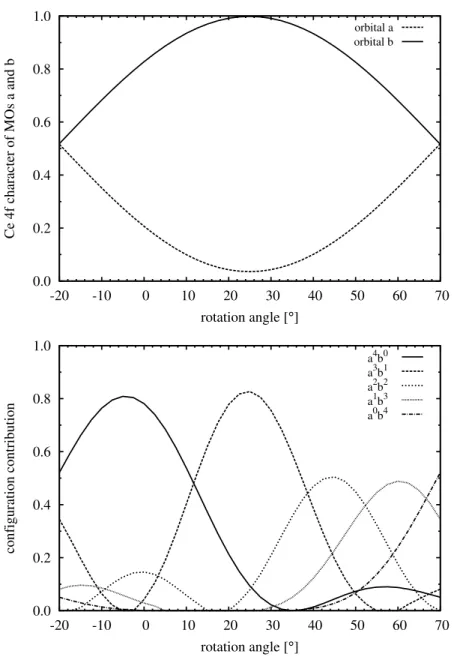
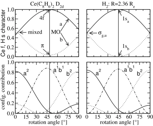
In the first part, the electronic structure of the ground state of several cerium complexes, Ce(C₈H₈)₂, Ce(C₈H₆)₂, Cp₂CeZ ( Z = CH₂, CH⁻, NH, O, F⁺) as well as CH₂CeF₂ and OCeF₂ were investigated. Using CASSCF computations including orbital rotations of the active orbitals, the underlying reason for the different interpretations of the cerium oxidation state (Ce(III) and Ce(IV)) of cerocene was found. By orbital rotation nearly pure cerium 4f and ligand π orbitals were obtained for cerocene. The CASSCF wavefunction based on these localized orbitals was analyzed and a leading f¹π³ was obtained.

Therefore, cerocene was classified as a Ce(III) compound. This result is in agreement to spectroscopic XANES data. Using the same computational technique, the electronic structure of all other cerium compounds was investigated. Similar to cerocene, nearly pure Ce 4f and ligand orbitals were obtained for Ce(C₈H₆)₂, Cp₂CeCH₂, Cp₂CeCH⁻ and CH₂CeF₂ resulting in a leading f¹π¹ or f¹p¹ configuration. Therefore these systems were classified as Ce(III) compounds. In contrast the complexes Cp₂CeNH, Cp₂CeO and OCeF₂ should be described as mixed valent Ce(III)/Ce(IV) compounds, whereas the Cp₂CeF⁺ complex can be categorized as a Ce(IV) compound. It can be shown that the most compact wavefunction, which correctly describes the influence of the Ce 4f orbitals can be obtained for all molecules, except cerocene, at the CASSCF(2,2) level.

These compact wavefunctions based on localized orbitals were used to investigate the nature of the orbital interactions of the active orbitals. The results revealed that the 4f-π orbital interaction of Ce(C₈H₆)₂ as well as the 4f-p orbital interaction of CH₂CeCp₂, CH⁻CeCp₂ and CH₂CeF₂ of the Ce-CH₂ or Ce-CH bonds can be classified as covalent interactions. The mixed valent systems revealed an increased ionic character of the active orbital interactions for the Ce-NH and Ce-O bonds, whereas the Ce-F bond can be clearly described as ionic. These results are in a good agreement to the assigned

(6)

oxidation states.

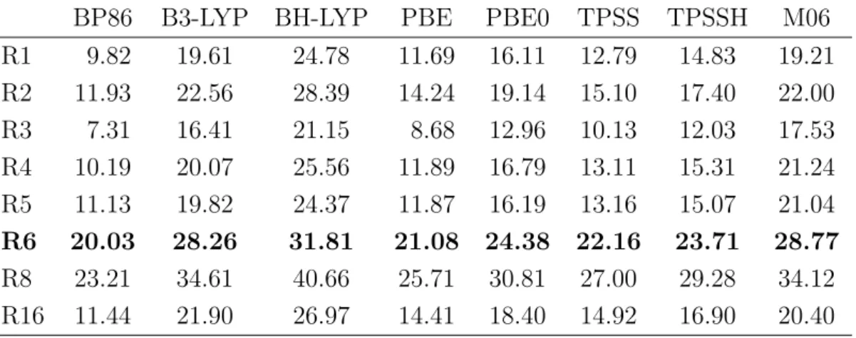
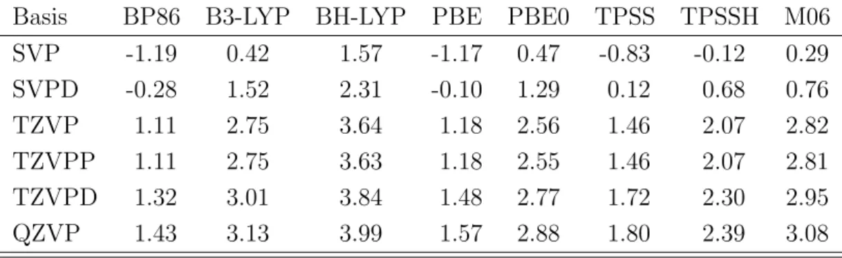
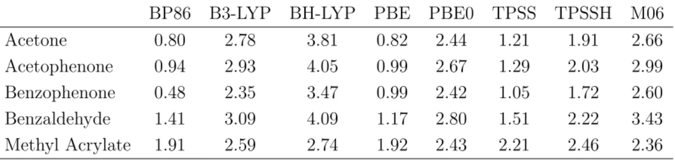
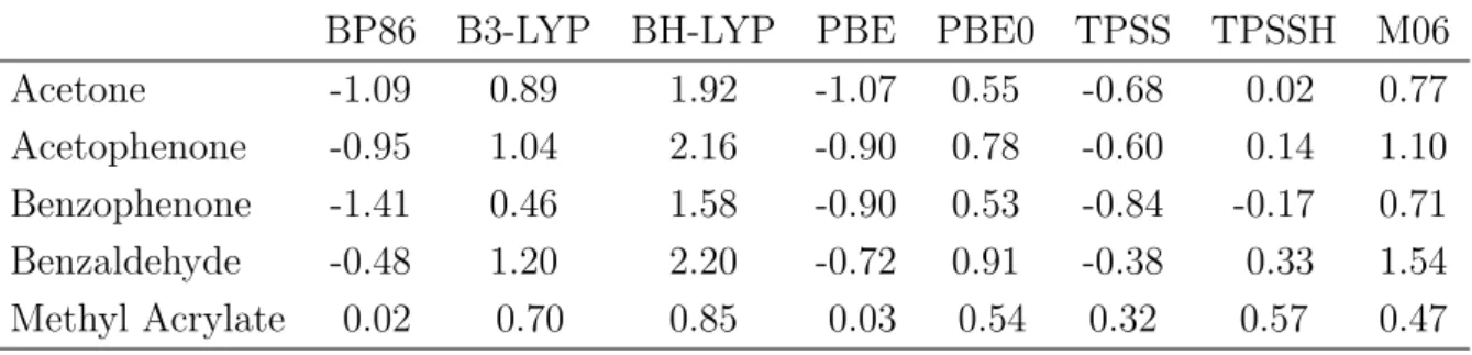
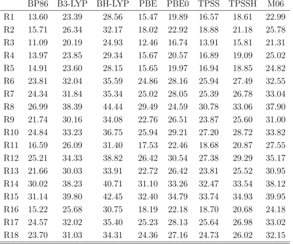
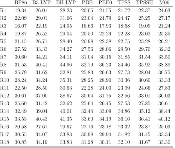
In the second part of this thesis, the quality and reliability of DFT computations of reactions compared to experimental results was investigated. The energies of the start- ing materials, the products as well as the transition states of several iodine catalyzed reactions were computed using various DFT methods. The results revealed that experimental outcomes (reaction time and product yields) can not be computed reliably for the whole set of investigated reactions. Additionally, it revealed that modern and older functionals possess the same predictive credibility. Nevertheless it was shown that all experimental outcomes of the reactions between methyl acrylate and aniline derivatives were reproduced by DFT methods. Therefore a reliable reaction prediction using DFT methods is not generally performable, but based on experimental results, DFT computations can predict reaction trends of very similar systems correctly. These correct predictions were obtained by all used functionals, which emphasizes that for a specific application modern and older functionals might possess the same quality.

(7)

Kurzzusammenfassung

Diese Arbeit untergliedert sich in zwei große Themenbereiche, die Untersuchung der Elektronenstruktur von Cer Komplexen im Hinblick auf die Bedeutung der 4f-Orbitale und der Klassifizierung des Oxidationszustandes des Cer-Ions in den chemischen Verbin- dungen, sowie der Untersuchung der Qualität von DFT Rechnungen im Hinblick auf die korrekte Reproduktion von experimentellen Ergebnissen und ihrer Einsatzfähigkeit im Bereich der Reaktionsprädiktion.

Im ersten Teil dieser Arbeiten wurde die Elektronenstruktur von verschiedenen Cer- Verbindungen, Ce(C₈H₈)₂, Ce(C₈H₆)₂, Cp₂CeZ ( Z = CH₂, CH⁻, NH, O, F⁺), sowie CH₂CeF₂ und OCeF₂ untersucht. Zunächst konnte mithilfe von CASSCF-Rechnungen in Kombination mit einer Orbitalrotation der aktiven Orbitale, die Ursache für die verschiedenen Interpretationen des Cer-Oxidationszustandes (Ce(III) und Ce(IV)) im Ce- rocen aufgeklärt werden. Anschließend konnten durch Entmischung der Molekülorbitale von Cerocen, Orbitale erzeugt werden, die entweder nahezu auschließlich 4f-Charakter des Cers oder π-Charakter der Liganden aufwiesen. Auf der Basis dieser Orbitale konnte die CASSCF-Wellenfunktion analysiert werden, wodurch sich eine führende f¹π³ zeigte und somit die Klassifizierung dieser Verbindung als Ce(III)-Komplex ermöglichte, welche konsistent zu den spektroskopischen XANES-Daten ist. An die Erkenntnisse des Cerocens anschließend, wurde die Elektronenstruktur weiterer, bereits genannter, Cer Komplexe analysiert. Es konnte hierbei gezeigt werden, dass vergleichbar zum Cerocen, die Molekülorbitale von Ce(C₈H₆)₂, Cp₂CeCH₂, Cp₂CeCH⁻ und CH₂CeF₂ ebenfalls in nahezu reine Cer 4f- und π- bzw. p-Ligandenorbitale überführt werden können. Durch eine folgende CASSCF-Wellenfunktionanalyse konnten diese Verbindun- gen ebenfalls als Ce(III)-Komplexe klassifiziert werden. Die weiteren Verbindungen zeigten ein abweichendes Verhalten. Die Komplexe Cp₂CeNH, Cp₂CeO und OCeF₂ konnten als gemischt-valente Ce(III)/Ce(IV)-Verbindungen klassifiziert werden. Die einzige Verbindung, die als Ce(IV)-Verbindung eingestuft werden konnte ist Cp₂CeF⁺, bei der die Bedeutung der Cer 4f-Orbitale vernachlässigbar war. Darüber hinaus konnte für alle Moleküle, außer Cerocen, eine kompakte CASSCF(2,2)-Wellenfunktion erhalten werden, ohne die korrekte Beschreibung der 4f-Orbitale zu verlieren. Diese Wellenfunk-

(8)

tion ermöglichte eine Untersuchung der Orbitalwechselwirkungen der aktiven Orbitale, wodurch gezeigt werden konnte, dass die 4f-π Orbitalwechselwirkung im Ce(C₈H₆)₂, sowie die 4f-p-Wechselwirkung der Ce-CH₂- bzw. Ce-CH-Bindungen in CH₂CeCp₂, CH⁻CeCp₂ und CH₂CeF₂ als kovalent eingestuft werden können Die gemischt valenten Cer Komplexe zeigten einen erhöhten ionischen Orbitalwechselwirkungscharakter bei den Ce-NH- bzw. Ce-O-Bindungen. Der Cp₂CeF⁺ Komplex zeigte eine eindeutige ion- ische Wechselwirkung der Ce-F-Bindung. Somit ist ebenfalls die Wechselwirkungsklas- sifizierung in Übereinstimmung mit den berechneten Oxidationszuständen.

Im zweiten Teil dieser Arbeit wurde die Qualität von DFT-Rechnungen und experimentellen Ergebnissen der organischen Synthese untersucht. Als Beispielsystem dienten verschiedene durch Iod katalysierte Reaktionen, deren Edukte, Produkte und Übergangs- zustände mit verschiedenen Methoden berechnet wurden. Es konnte hierbei gezeigt werden, dass eine verlässliche Übereinstimmung mit den experimentellen Ergebnissen (Reaktionszeit und Ausbeute) nicht über die gesamte Anzahl an untersuchten Ergebnis- sen erhalten werden kann. Weiterhin konnte gezeigt werden, dass moderne und ältere Funktionale eine ähnliche Aussagekraft auf die Prädiktion haben. Eindeutige verlässliche Ubereinstimmung mit den experimentellen Ergebnissen konnten nur innerhalb der Reak-¨ tionen erhalten werden, die Anilinderivate mit Methyacrylat umsetzten. Somit konnte geschlussfolgert werden, dass eine richtige Vorhersage von Reaktionsausgängen nicht uneingeschränkt möglich ist, jedoch ausgehend von experimentellen Erkentnissen ist es möglich chemisch sehr ähnliche Reaktionen richtig vorherzuberechnen. Diese Vorhersage ist mit allen verwendeten Funktionalen möglich, wodurch gezeigt wurde, dass moderne Funktionale bei einer spezifischen Anwendung keine bessere Qualität als ältere Funk- tionale aufweisen müssen.

(9)

1 Introduction

Over the last decades computational chemistry became an important part of the chemical scientific community in general. A huge variety of computational methods arised, which can be mainly divided into wave function-based methods, density functional theory methods and molecular mechanics. These methods are used in all fields of chemistry, e.g. simulating spectra, computing bond distances, finding the most stable confomer of a molecule or investigating reaction mechanisms. In principle, any measurable value can be calculated by computational methods. According to the physical complexity of chemical systems, all developed and applied methods are approximations of the exact description. Therefore, the results obtained by computations as well as conclusions based on these results should be treated with caution and need to be checked. Nevertheless, quantum chemistry can be used to support experimental research and to derive insights for chemical systems, where suitable experiments are not available.

In this work, computational methods are used to investigate the electronic structure of cerium complexes in order to assign reasonable oxidation states to cerium and to point out the relevance of the 4f orbitals in these compounds. The concept of oxidation states is fundamental in chemistry, but especially for multi-reference systems it is not well defined. Therefore, a suitable procedure for the assignment of oxidation states for such systems, using wave function-based methods, will be presented and discussed.

For large systems density functional theory methods have to be used, according to the huge computational demand of highly accurate wave function-based methods. Many DFT computations are performed to support an experimental outcome and are performed after the experimental results were obtained. Predictive DFT computations are rare. However, one target of computational chemistry is to develop methods, which can be used to correctly predict reaction outcomes. In order to investigate the correctness of DFT computations, several iodine catalyzed reactions were computed with a variety of available standard DFT functionals. The results, paying special attention on the correctly computed experimentally observed outcomes and trends, will be discussed.

(14)

Introduction

(15)

2 Theory

For not explicitly time-dependant Hamiltonians the fundamental task of theoretical chemistry is to solve the Schr¨odinger equation for a specific quantum mechanical system. An exact solution of this equation is solely possible for the hydrogen atom or hydrogen-like systems, whereas more complex quantum chemical systems have to be solved approximately. This difficulty lead to various approaches and methods for the approximate solution of the Schr¨odinger equation. In the following sections, the concepts of quantum chemistry and main aspects of common approaches will be outlined.

The discussions and fundamental formulas given in the following chapter mainly follow the book of Szabo and Ostlund [1], Jensen [2] as well as the book of Levine and Helgaker [3]. For a compact description of the corresponding equations, atomic units are used, implying that the reduced Planck’s constant, the elementary charge, the rest mass of the electron as well as the Coulomb force constant are set to the numerical value of one (i.e. ~=e=m_e = _4π¹

0 = 1).

2.1 Schr¨odinger Equation and the Form of the Hamiltonian

The most basic equation of nonrelativistic quantum chemistry is the time-dependent Schr¨odinger equation. For an hydrogen atom it can be written as

i~∂

∂t

Ψ(~x, t)

= ˆH

Ψ(~x, t)

. (2.1)

H: Hamiltonianˆ Ψ: Wave function

~

x: Vector of the spatial coordinates and the spin of the electron t: Time

Equation (2.1) describes the state of a quantum chemical system at any time t en- tirely. Any property can be derived by applying the corresponding operator to the wave function, e.g. ˆH for the energy of the system.

(16)

2.1 Schr¨odinger Equation and the Form of the Hamiltonian Theory

The time dependency can be separated by using a product ansatz of the wave function with a time-dependent function Θ(t) and function Ψ(~x), which depends on the spatial coordinates and the spin of the electrons

|Ψ(~x, t)

= Θ(t)|Ψ(~x)

. (2.2)

Combining the equations (2.1) and (2.2) leads to the differential equation

i~

∂

∂tΘ(t) = EΘ(t), (2.3)

where E is the energy of the system and which has to be solved to obtain the time- dependent part of the wave function. The resulting formula is given by

Θ(t)∝exp

−iEt

~

. (2.4)

After applying this separation ansatz, the time-independent Schr¨odinger equation is obtained as

Hˆ Ψ(~x)

=E Ψ(~x)

, (2.5)

constituting the most important equation in the field of non-relativistic quantum chemistry according to the fact that most applications treat stationary states and properties.

The Hamiltonian includes the physics of a system, for instance in the case of a molecule in the non-relativistic case the operator is constructed from the kinetic energy of the electrons Ekin(e), the kinetic energy of the nuclei Ekin(nuc), the electron-electron repulsion Epot(e,e), the electron-nuclei attraction Epot(e,nuc) and the repulsion of all nuclei Epot(nuc,nuc) and is given by following equation (2.6)

Hˆ =E_kin(e) +E_pot(e,e) +E_pot(e,nuc) +E_pot(nuc,nuc) +E_kin(nuc)

=−1 2

n

X∆i+

n

X 1 r −

n

X

N

XZ_I r +

N

XZ_IZ_J r − 1

2

N

X 1

M ∆I. (2.6)

(17)

Theory 2.1 Schr¨odinger Equation and the Form of the Hamiltonian

Z_I: Nuclear charge of atomI

r_ij: Distance of the particles iand j

In principle the Schr¨odinger equation (2.5), using the Hamiltonian shown in equation (2.6), has to be solved for the electrons and the nuclei for a molecular quantum system.

As a consequence, the total wave function is a function constructed from an electronic and a nuclear part. The Born-Oppenheimer approximation states that the wave function of the nuclei and the wave function of the electrons can be separated by applying a product ansatz

Ψ_total= Ψ_elec·Ψ_nuc. (2.7)

Since the mass of the nuclei in comparison to the electron’s is much larger, the nuclei are assumed to be fixed at their local coordinates. Therefore the kinetic energy of all nuclei can be assumed to be zero and the repulsion energy of the nuclei can be added as a constant for a specific geometrical arrangement of the investigated molecule. This results in the following equation, that constitutes a simplified form of the Hamiltonian,

Hˆ_el=−1 2

n

X

i=1

∆_i+

n

X

i<j

1 r_ij −

n

X

i=1 N

X

I=1

ZI

r_iI, (2.8)

that is often referred to as the electronic Hamiltonian ˆH_el and is used in many computational methods in quantum chemistry.

(18)

2.2 The Hartree-Fock Method Theory

2.2 The Hartree-Fock Method

Due to the interaction of electrons in instantaneous motion, the Schr¨odinger equation can not be solved exactly for many-electron systems. According to this problem, many computational methods intend to calculate an approximate solution of the Schr¨odinger equation. One fundamental approach is the Hartree-Fock (HF) method that nowadays is the basis for many so-called correlation or post Hartree-Fock methods and approaches, e.g. configuration interaction (CI) or coupled cluster (CC).

The wave function ansatz of the HF approach is a single determinant composed of one electron wavenfunctions named spin orbitals. This wave function ansatz is usually called Slater determinant [4] and can be written as

|Ψ(~x₁, ~x₂, . . . , ~x_n)

=

Ψ(1,2, . . . , n)

= 1

√n!

φ₁(1) . . . φ₁(n) ... . .. ... φ_n(1) . . . φ_n(n)

. (2.9)

n: Number of electrons φ_i: i-th spin orbital

The Pauli exclusion principle states that the wave function of electrons, fermions in general, has to be antisymmetric under the exchange of two arbitrary particles

Ψ(1, . . . , i, . . . , j, . . . , n) =−Ψ(1, . . . , j, . . . , i, . . . , n). (2.10) The Slater determinant satisfies this antisymmetry requirement.s

The Schr¨odinger equation (2.5) is solved approximately in the HF approach[1] by using one Slater determinant and the electronic Hamiltonian presented in equation (2.8)

Hˆ Ψ˜

≈E Ψ

. (2.11)

To obtain the approximate solution, the expectation value of the energy E

, defined by

hEi= Ψ

Hˆ_el Ψ Ψ

Ψ , (2.12)

(19)

Theory 2.2 The Hartree-Fock Method

The variation principle guarantees that the approximate solution and the resulting energy is an upper bound to the exact energy. This also ensures that a solution with a lower energy provides a more accurate solution and description for the quantum chemical system.

The minimization process is performed using the method of Lagrange multipliers under the additional restriction of orthonormalized spin orbitals

hφ_i|φ_ji=δ_ij (2.14)

and leads to the so-called canonical Fock equations

fˆ1φi(1) =εiφi(1). (2.15) The main advantage of this method is that the Schr¨odinger equation with ann-particle wave function is reduced to n one particle equations, which can be solved more easily.

The Fock operator ˆf₁

fˆ₁ =−1 2∆₁−

N

X

I=1

Z_I r_1I +

n

X

j=1

hJˆ_j(1)−Kˆ_j(1)i

, (2.16)

Jˆ_j: Coulomb operator Kˆ_j: Exchange operator

is an effective one-electron Hamiltonian that computes the spin orbital energy _i for the corresponding spin orbital φ_i. The Fock operator is constructed by an one-particle part

ˆh(1) =−1 2∆₁−

N

X

I=1

Z_I

r_1I (2.17)

and a two-particle part, containing the Coulomb and exchange operators, which describes the electron-electron interaction in an averaged way.

The Coulomb operator can be interpreted as the classical Coulomb interaction, whereas the exchange operator has no classical analogue and is mathematically derived from the antisymmetry requirement of the wave function, resulting from the Pauli exclusion principle. These operators are defined by acting on an orbital in the following form:

Jˆ_jφ_i(1) = Z

φ^∗_j(2) 1 r12

φ_j(2)dτ₂φ_i(1) (2.18) Kˆ_jφ_i(1) =

Z

φ^∗_j(2) 1

r₁₂φ_i(2)dτ₂φ_j(1). (2.19)

(20)

2.2 The Hartree-Fock Method Theory

J_j: Coulomb operator K_j: Exchange operator

Expectation values of these operators occur as the so-called Coulomb- and exchange integrals. These integrals are calculated as [1]

J_ij =hφ_i|Jˆ_j|φ_ii= Z Z

φ^∗_i(1)φ^∗_j(2) 1 r12

φ_i(1)φ_j(2)dτ₁dτ₂ (2.20) K_ij =hφ_i|Kˆ_j|φ_ii=

Z Z

φ^∗_i(1)φ^∗_j(2) 1

r₁₂φ_j(1)φ_i(2)dτ₁dτ₂. (2.21) J_ij: Coulomb integral

K_ij: Exchange integral

After deriving the Fock equations (2.15), this set of integro-differential equations needs to be solved in the HF approach. Therefore each orbital has to be expanded in a linear combination of basis functions. This ansatz is related to the mathematical fact that each function can be, in principle, approximated as a linear combination of different functions. A specific amount of basis functions defines a basis set. This ansatz is exact in case of a complete basis set.

The spin orbitalsφ_i are generally constructed by a spatial functionϕ_i and a spinfunction ω_i, which is given by

φ_i(~x) =ϕ_i(x, y, z)·ω_i({α, β}). (2.22) The integration over the spin coordinates is computed as

α α

= β

β

= 1 (2.23)

α β

= β

α

= 0. (2.24)

The spatial part of the spin orbitals is approximated by a linear combination of the basis functions χ_i, for wich Gaussian functions are most commonly used

ϕ_i =

mbasis

X c_αiχ_α. (2.25)

(21)

Theory 2.2 The Hartree-Fock Method

The orbital coefficents c_αi need to be optimized with respect to the energy to finally solve the Schr¨odinger equation approximately. By multiplication from the left with an additional basis function χ_β and formulating an expectation value for each orbital leads to a matrix representation named Roothaan-Hall equation

F C =SCε. (2.27)

F: Fockmatrix with matrix elements Fαβ =hχα|f|χˆ βi

C: Coefficient matrix (i-th column corresponds to the coefficients for the i-th orbital) S: Overlap matrix with matrix elements Sαβ = hχα|χβi

ε: Matrix of the spinorbial energies εii=εi in the canonical HF Under the constraint of orthonormalized basis functions

hχi|χji=δij, (2.28)

the overlap matrix transforms into the identity matrix and the Roothall-Hall equation simplifies to the following form

F C =Cε, (2.29)

which is usually solved in an iterative manner by the self-consistent field (SCF) procedure. The iterative computation of the orbital coefficients is needed, because the Coulomb- and exchange operatos in the Fock operator depend on the orbitals them- selves. The total HF energy is calculated by

E_HF=

n

X

i=1

ε_i−X

i>j

(J_ij −K_ij) +E_pot(nuc,nuc). (2.30) The summation of the orbital energies double counts the electron-electron interaction, which is corrected by the second term in equation (2.30) and the nuclear repulsion energy has to be taken into account for a specific geometry. The HF method does not deliver the exact energy, even for an infinite or complete basis set, the energy reaches the so-called Hartree-Fock limit. The HF method computes approximately 99% of the exact energy for a quantum chemical system. This accuracy is not sufficient for many applications and therefore the HF approach is only the basis for many more elaborate computational methods, which are described in the following section.

(22)

2.3 Correlation Methods Theory

2.3 Correlation Methods

As discussed, the HF method can not deliver the exact energy. This is caused by approx- imating the wave function as a single determinant and describing the electron-electron interaction by means of an averaged field. In order to obtain the exact nonrelativistic energy, the interaction of every electron pair has to be described correctly, which is called electron correlation and the missing energy amount is named correlation energy. The correlation energy is always a negative value, because the HF energy is an upper bound to the exact energy. It is defined by the difference of the HF energy and the exact energy

E_corr =E_exact−E_HF, (2.31)

and can be computed using different approaches. The fundamental concepts of the correlation methods as well as the advantages and disadvantages of these methods are discussed in the following subsections.

2.3.1 Configuration Interaction

An elaborate approach of computing the correlation energy is the configuration interaction (CI) method. The basic idea is to choose a linear combination of Slater determinants as the wave function ansatz to approximately solve the Schr¨odinger equation. This wave function ansatz can be mathematically written in the following form

|Ψ_CIi=k_ref|Ψ_refi+X

ia

k_i^a|Ψ^a_ii+X

i<j a<b

k^ab_ij Ψ^ab_ij

+· · · . (2.32)

This type of wave function ansatz is conceptionally very similar to the basis set approximation in the Hartree-Fock method described in equation (2.25). Therefore, the common nomenclature of the one particle basis, which is the basis set{φ_i}and the many-particle basis, which contains the Slater determinants {|Ψ_ii}in the CI expansion, is often used.

The many-particle basis consists of a reference determinant |Ψ_refi,which normally corresponds to the HF determinant Ψ_HF, also often referred to as Ψ₀ and a specific set of

(23)

Theory 2.3 Correlation Methods

terminology is used to categorize different CI approaches by their substitution order, e.g. a CI calculation which includes all singles and doubles is therefore called CISD.

Inserting this ansatz into the Schr¨odinger equation leads to the equation

H~k_ν =E_CI,ν~kν, (2.33)

H: Hamilton matrix with matrix elements H_ij = Ψ_i

Hˆ Ψ_j

~k: Coefficient vector for the ν-th state

E_CI: Ground state energy of the CI approach

for the ground state. The variation principle is also valid for the CI method, so a reduction of the energy guarantees a better solution of the Schr¨odinger equation and a higher quality of the approximate wave function. The Hamilton matrix in the CI approach can be visualized in the following way

Ψ₀

S

D

T Q

· · · Ψ₀

Ψ₀ Hˆ

Ψ₀

0

Ψ₀ Hˆ

D

0 0 · · ·

S

S Hˆ

S S

Hˆ

D S

Hˆ T

0 · · · D

D Hˆ

D D

Hˆ T

D Hˆ

Q

· · · T

T Hˆ

T T

Hˆ Q

· · · Q

Q Hˆ

Q

· · ·

... ...

(2.34)

In this form a few rules, which are simplifying the computation can be seen. First, there is no coupling between the reference determinant and the single excitations, which was stated by the Brillouin’s theorem for HF orbitals. Due to the fact that singles mix with the double excitations and the doubles interact with the reference determinant, the singles can not be neglected in a CI calculation. The effect of the singly excited Slater determinants on the total energy is indirect. The second rule which can be observed is that all matrix elements between determinants differing in more than two orbitals also vanishes. This is an enormous reduction of the elements, which need to be determined, especially in CI calculations including a high substitution level. The third and last simplification is the consequence of the hermiticity of this matrix, which states that H^∗_ij =H_ji are equal. Therefore only the upper triangle of this matrix has to be determined. In principle, the CI method is able to compute the exact nonrelativistic energy of a quantum chemical system. This can be achieved by using an infinite one particle basis and including all possible determinants in the CI wave function ansatz, which is named full configuration interaction (FCI). For a finite one particle basis, the maximum reachable quality by using the FCI method is called the FCI limit. According

(24)

to the huge number of upcoming determinants, that are determined by N_dets= K

n

!

= K!

n! (K−n)!, (2.35)

K: number of spin orbitals n: number of electrons

the FCI method is only applicable for about 10 electron systems, while using a double zeta basis set. Therefore the wave function has to be truncated. The most used CI method is the already mentioned CISD, but also CISDT or CISDTQ methods can be used for small systems nowadays.

The CI method can compute good results for specific tasks where the HF approach is conceptionally failing. A famous example is the dissociation of the H₂ molecule. In this homonuclear diatomic compound the molecular orbitals (MOs) are linear combinations of the 1s orbitals of the hydrogen atoms given by

σg = 1sA+ 1sB (2.36)

σ_u = 1s_A−1s_B, (2.37)

if the normalization constants are neglected. The Slater determinant for the H₂molecule, composed of two hydrogen atoms H_A and H_B can be constructed from the binding σ_g MO for the ground state

Ψ_H₂

∝σ_g^α(1)σ_g^β(2)−σ_g^α(2)σ_g^β(1). (2.38) Separating the spin and the spatial function of this wave function results in

Ψ_H₂

∝σ_g(1)σ_g(2) α(1)β(2)−α(2)β(1)

. (2.39)

From the spatial part of the wave function the inability of the HF ansatz to describe the dissociation can be seen. Inserting equation (2.37) into the spatial part results in

σ_g(1)σ_g(2) = 1s_A(1) + 1s_B(1)

1s_A(2) + 1s_B(2)

(2.40)

= 1s (1)1s (2) + 1s (1)1s (2) + 1s (1)1s (2) + 1s (1)1s (2) (2.41)

(25)

energy will have a low quality using the HF method. The CID method has the ability to describe this phenomenon correctly. The doubly excited determinant constructed from the antibonding σ_u orbitals results in

σ_u(1)σ_u(2) = 1s_A(1)1s_A(2) + 1s_B(1)1s_B(2)−1s_A(1)1s_B(2)−1s_B(1)1s_A(2). (2.42) The CID wave function can then be written as

ΨCID

= k1σg(1)σg(2) +k2σu(1)σu(2)

α(1)β(2)−α(2)β(1)

, (2.43) and by choosing the coefficients as

k1 =−k2, (2.44)

the ionic terms in the wave function vanish and the wave function will only be composed of the covalent terms, which are needed at the dissociation limit of the H2 dimer

ΨCID

=k1 1sA(1)1sB(2) + 1sB(1)1sA(2)

α(1)β(2)−α(2)β(1)

. (2.45)

The CI ansatz is not size-consistent in general if the excitation level is truncated. This is the main disadvantage of this approach, because size-consistency is an important attribute for a correlation method in general. Therefore, the basic idea of size-consistency will be illustrated briefly. For a system ABcomposed of two non-interacting subsystems A and B the Hamiltonian is separable

HˆAB = ˆHA+ ˆHB, (2.46)

as a logical consequence of the absent interaction. Therefore the total energy should be the summation of the two energies of the subsystems A and B

E_AB =E_A+E_B. (2.47)

Considering the CISD method for such a case reveals that double excitations are included in the separated calculations for the subsystems A andB, which results in the inclusion of quadruple excitations for the summation of these two systems. The CISD method applied to the combined system AB however, uses only the double excitations, which results in a different quality. According to this it can be concluded that the CISD method is not size-consistent, which can be problematic for several applications, e.g. reaction energies. The fundamental size-consistency problem has been overcome by the well known and often used coupled cluster ansatz that will also be presented and discussed in throughout the following sections.

(26)

2.3.2 Multi-configurational Self-consistent Field

Electron correlation is generally divided into two different types, dynamic and static correlation. The previously explained CI approach is in general suitable for quantum chemical systems that have one dominant leading Slater determinant. This type of electron correlation is named dynamic correlation. Static correlation is of special importance for multi-reference (MR) compounds, in which no single determinant is leading in the wave function. Well known examples are open-shell systems, transition states or excited states. The optimized orbitals of the HF method are not appropriate for these kinds of MR systems and the orbitals have to be generated using a different approach. The multi- configurational self-consistent field (MCSCF) approach overcomes this problem and is suitable for MR systems. The general wave function ansatz is a linear combination of determinants, which is analogue to the CI wave function

|Ψ_MCSCFi=X

I

k_I|Ψ_Ii. (2.48)

In contrast to the CI method, where the orbitals are not optimized, the MCSCF method optimizes the coefficients of the determinants and the orbital coefficients. The MCSCF method becomes identical to the HF approach, if only one Slater determinant is used.

As well as the CI method the MCSCF approach, except CASSCF, is not size-consistent entailing the same problems, which were already highlighted for the CI method. Nev- ertheless MCSCF can be used for many applications, e.g. excitation energies for atoms and molecules, delivering very accurate results. The main disadvantage and problem of MCSCF is the choice of the determinants that are included in the wave function ansatz.

The determinants need to be carefully selected, motivated by chemical or physical understanding of the investigated systems. An unbalanced or uncarefully picked set of determinants can lead to inaccurate results or wrong insights.

In the beginning of the MCSCF method, the determinants were individually selected.

Nowadays more systematic approaches, e.g. complete active space self-consistent field (CASSCF) or restricted active space self-consistent field (RASSCF), are used. In these methods the determinants are chosen systematically, defined by the so-called active space. In this systematic approach the orbital space is partitioned into three different subspaces which are namely the inactive, virtual and active orbitals. This partitioning

(27)

In general the orbitals are categorized in the following way:

• inactive orbitals: Orbitals that are usually energetically low and are therefore always occupied in all used determinants of the wave function expansion.

• virtual orbitals: Orbitals that are, in contrast to the inactive orbitals, energetically high and therefore always unoccupied in all determinants that are used in the wave function expansion.

• active orbitals: These orbitals define the varying occupation patterns of the determinants which are included in the CI expansion of the MCSCF method.

Commonly these orbitals correspond to the highest occupied molecular orbitals (HOMOs) and the lowest unoccupied molecular orbitals (LUMOs) determined by the HF method.

The active orbitals can and should be selected by a rational understanding of the system and not only according to the HF orbital energies, especially for open-shell systems. For a quantum chemical open-shell system, e.g. vanadium, that has an electron configuration of [Ar]3d³4s², all determinants resulting from the d-orbitals should be included in the wave function regardless of the HF orbital energies of the d-orbitals. Such a procedure is the basic idea of the CASSCF method. After dividing the orbital space to the already mentioned subspace, all determintans which arise from the active orbitals and electron will be included in the CI expansion to construct the wave function. The resulting number of determinants can be calculated according to the FCI approach

N_dets= K_act n_act

!

= K_act!

n_act! (K_act−n_act)!. (2.49) K_act: Number of spin orbitals included in the active space

n_act: Number of electrons included in the active space

Therefore the CASSCF method is often described as a FCI approach in the active orbital space and the qualitively correct energies for specific applications like excitation energies becomes clear. For small active spaces this approach should be the best method to derive accurate electronic energies and corresponding results, but for systems where larger active spaces are needed a different approach might be needed.

The RASSCF approach is such a method and the basic idea of this procedure is to divide the whole orbital space into more subspaces. The virtual and inactive orbitals are defined equivalently to the already given definition. In the RASSCF approach, the active space is partitioned into three subspaces. In contrast to the CASSCF method not

Interpretation of ab initio Calculations of Cerium Compounds and Predictive Power of Density Functional Theory Calculations for Iodine Catalysis

Abstract

Kurzzusammenfassung

Contents

1 Introduction

2 Theory