Physical Kinetics
Prof. Dr. Igor Sokolov
Email: sokolov@physik.hu-berlin.de
July 10, 2019
Contents
1 Fluctuations close to equilibrium 4
1.1 General discussion . . . 4
1.2 Prerequisites: Probability theory . . . 6
1.3 Multivariate Gaussian distributions . . . 9
1.4 Fluctuations of thermodynamical properties . . . 11
2 Onsager’s Theory of Linear Relaxation Processes 13 2.1 Relaxation to equilibrium . . . 14
2.2 Relaxation of fluctuations . . . 18
2.3 Microscopic reversibility and symmetry of kinetic coefficients . . . 19
2.4 Simple examples . . . 21
2.4.1 Example 1: Heat transport . . . 21
2.4.2 Example 2: Mass transport . . . 22
2.4.3 Example 3: Thermoelectric phenomena . . . 23
2.5 Continuous systems . . . 24
2.5.1 Heat equation and diffusion equation . . . 24
2.5.2 The Fokker-Planck equation and the Einstein’s relation . . . 28
2.5.3 General hydrodynamic description . . . 31
3 Fluctuations and dissipation 41 3.1 Linear response to an external force . . . 41
3.2 Response function . . . 43
3.3 Spectrum of fluctuations . . . 44
3.3.1 Fluctuation-Dissipation Theorem in Fourier representation . . . 45
3.4 More on random processes. . . 46
3.4.1 Some definitions concerning random processes: Ergodic hierarchy. . . 46
3.4.2 Conditions for ergodicity. . . 47
3.4.3 The Wiener-Khintchine Theorem . . . 48
3.5 Fluctuations and noise . . . 50
4 Brownian motion 52 4.1 Historical overview . . . 52
4.2 The Langevin’s original approach . . . 52
4.3 Taylor (Green-Kubo) formula . . . 54
4.4 Overdamped limit . . . 56
4.5 From Langevin equation to Fokker-Planck equation I . . . 57
4.5.1 Generalization to higher dimensions . . . 59
5 Another approach to the Fokker-Planck equation 60 5.1 Einstein’s theory of Brownian motion . . . 60
5.2 Equations for the probability density . . . 61
5.3 Stochastic integration . . . 64
5.3.1 The problem of interpretation . . . 66
5.4 Transition rates and master equations. . . 71
5.5 Energy diffusion and detailed balance . . . 73
6 Escape and first passage problems 75
6.1 General considerations . . . 76
6.2 Mean life time in a potential well . . . 77
6.2.1 The flow-over-population approach . . . 77
6.3 Rates of transitions . . . 80
6.3.1 The Arrhenius law . . . 80
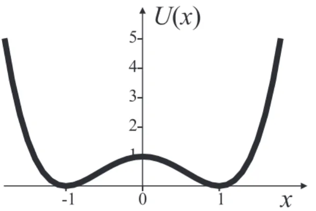
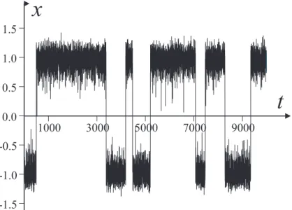
6.3.2 Diffusion in a double-well . . . 80
6.4 Kolmogorov backward equation . . . 82
6.4.1 Pontryagin-Witt equations . . . 83
6.5 The renewal approach. . . 86
6.5.1 Example: Free diffusion in presence of boundaries . . . 88
6.6 An underdamped situation . . . 89
7 Simple bath model: Kac-Zwanzig bath 92 8 The Boltzmann equation 98 8.1 The BBGKY-Hierarchy . . . 98
8.2 Single-particle distribution function . . . 101
8.2.1 Kinetic models . . . 102
8.3 The Boltzmann equation . . . 104
8.3.1 Maxwell’s transport equations . . . 105
8.3.2 Collision invariants . . . 107
8.3.3 The H-Theorem . . . 108
8.4 Relaxation time approximation for hydrodynamics: The BGK equation . . . 110
9 Kinetics of quantum systems 115 9.1 The Golden Rule . . . 115
9.2 Quantum mechanical Master equations . . . 117
9.3 Electron transfer kinetics . . . 122
9.4 The density matrix approaches . . . 125
9.4.1 The density matrix and the quantum Liouville equation. . . 125
9.4.2 Two level systems in the bath. . . 128
9.5 Master equation from density matrix approach. . . 138
1 Fluctuations close to equilibrium
1.1 General discussion
We start our considerations by a discussion of fluctuations in TD systems close to equilibrium, which will then allow us for introducing many important notions and notation, which will be useful for the discussion of non-equilibrium situations.
Although in a system in the state of TD equilibrium the TD-parameters (e.g. T, p, V, ...) do not change on the average or in a longer run, the molecular motion causes fluctuations in the values of the corresponding parameters. These fluctuations appear and dissolve, are typically small in the macroscopic parts of the system, but can be perceptible and important if a small subsystem is considered. As an example let us consider a small cylinder with a piston filled by a gas and immersed into the bath filled by the same gas at the same temperature and pressure. Due to molecular impacts the positionX of the piston (which translates from the volume of the gas inside the cylinder) will fluctuate. Assuming the motion of molecules to be “chaotic” (in the Boltzmann’s sense), we can then describe thisX(t) as arandom process. If we only concentrate on the result of a single-time measurement, X can be considered as arandom variable, and we can put a question, what is the probability (density) to measure some particular value of X.
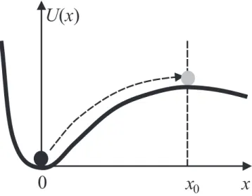
We discuss the Einstein’s approach to such fluctuations, based on the inversion of the Boltz- mann’s formula for microcanonical entropy. Let us consider our system (or a part thereof), which will be called a “body”, to be in contact with a bath; the whole system, consisting of the body and the bath (which will be called a “compound”) will be considered as isolated. If the fluctuations are “small” (i.e. the system stays close to equilibrium), its state even in the case of fluctuation can be described by a set of relevant thermodynamical variables (e.g. S, T, p, V, ...). The existence of fluctuations implies that the entropy of the system is not always maximal (i.e. that the system is not always in its “most probable” state), but that it might depart from it to a less probable one, and then return. This entropy is still the function of thermodynamical parameter of the body and of the bath.
Let X be some parameter of the body, say, its volume, or electric charge, or magnetization, etc. (in our example above it is the coordinate of the piston which is translated from the volume), taking the value X0 in equilibrium. Let us assume that we can define the total entropy of the composite Sc as a function of this X. Since the entropy of an isolated system at equilibrium attains its maximum, we have
Sc(X) =Sc(X0) + 1 2
∂2Sc
∂X2(X−X0)2, (1)
if we assume that the maximum is a simple quadratic one (no phase transitions!). The correspond- ing second derivative ∂X∂2S2 is therefore negative. Let us denote it by −γ =−δ2.
Since the total entropy is connected with the number W of microstates and therefore with the probability p∝W of the corresponding macrostate as
S =kBlnW =const·kBlnp,
by inverting this relation we getW = exp(Sc/kB). The probability to find a particular (macro)state compatible with the corresponding restrictions is then proportional to the corresponding W, so that the probability to find a fluctuation lowering the total entropy by amount ∆Ss is
p∝exp ∆Sc
kB
.
with ∆Sc =Sc(X)−Sc(X0), or
p∝exp
− γ
2kB(X−X0)2
, i.e. is a Gaussian distribution. Here
γ =− ∂2S
∂X2 X=X0
>0 (2)
where we assume that the entropy at equilibrium reaches its simple quadratic maximum. It is important to note that the Gaussian nature has to do with the fact that the total entropy is expanded close to equilibrium, far from the points of phase transitions, and that the value of X−X0 is small. Gaussian fluctuations are universally observed close to equilibrium under such restrictions, but there are no reasons to look for Gaussian fluctuations in non-equilibrium systems or close to phase transition points. Large deviations also may not follow the Gaussian law. Up to now we have no idea how to calculate γ. Here we follows a somewhat old-fashioned way of discussion; another approach can be found in1.
We assume, that the state of the whole system does not depend on whether the particular state of the body appeared as a spontaneous fluctuation, or was prepared on purpose as long as the total energy of the system does not change (it is fixed to be Ec as it is in the case when we considered an isolated system). To prepare the corresponding state on purpose we have to perform (reversible) workR on the body and (reversibly) remove the corresponding amount of energy from the bath, in the form of heat: ∆Ec = R+Q = 0. Since the system as a whole is at a constant temperatureT (it mostly consists of the bath) we haveQ=T∆Sc, so thatT∆Sc+R = 0, and the total change in entropy is ∆Sc=−R/T. Recalling the connection of the entropy with the number of microstates and therefore with the probability p∝W we have
p∝exp ∆Sc
kB
= exp
− R kBT
. (3)
We now calculate R provided the internal energy of the body, its volume and entropy, as well as external pressure and temperature are known. According to the First Law we have: ∆E = Abody +Qbody =R−p∆V +T∆S. (All quantities without subscripts are those of the body. Note that the total work performed with the body is notR, butR−p∆V since the bath also performs work, at least in the case when the volume of the body changes). Thus,
R= ∆E+p∆V −T∆S.
Here p and T are equilibrium values of the pressure and of the temperature of the body, equal to those of the bath. In what follows we denote them by p0 and T0 in order to distinguish them from probably fluctuating local values2. Note that for more complex bodies there might be further terms including, say, magnetization, or the number of particles, etc. Our thermodynamical approach generates therefore a quite general formalism.
We thus get:
p∝exp
−∆E+p0∆V −T0∆S kBT0
.
1 See e.g. W. G¨opel, H.-D. Wiemh¨ofer, Statistische Thermodynamik, Spectrum Verlag, 2000
2A question about fluctuations of temperature and other intensive parameters is somewhat tricky. If you want to learn (much) more, see M. Falcioni et al., Am. J. Phys.,79, 777-785 (2011).
We now note that since dE = −pdV +T dS the first non-vanishing contribution in enumerator appears in thesecond order in ∆V and ∆S: we expand ∆E =E(S+ ∆S, V + ∆V, ...)−E(S, V, ...) up to the second order in changes of its natural variables and get
p∝exp
− 1 kBT0
1 2
∂2E
∂V2(∆V)2+ ∂2E
∂V ∂S∆V∆S+ 1 2
∂2E
∂S2(∆S)2
. (4)
In general, if (V, S, ...) is a vector of relevant extensive variables describing the body, and x = (∆V,∆S, ...) is a vector containing their deviations from the equilibrium values, the total structure of the probability density of fluctuations is
p∝exp(−12xMx) (5)
where the matrix M has elements
mij = 1 kBT0
∂2E
∂xi∂xj,
i.e. is real and symmetric. Since the equilibrium situation corresponds to the maximal probability (i.e. maximal entropy) and is stable, the matrix is positively defined. Eq.(5) with the corresponding positively defined matrix corresponds to a multivariate Gaussian distribution.
In what follows, the matrix of the second derivatives if the total entropy with entries γij =− ∂2Sc
∂Xi∂Xj
Xi,j=(Xi,j)eq
= 1 T0
∂2E
∂Xi∂Xj =kBmij, (6) will be denoted by γ.
1.2 Prerequisites: Probability theory
What you had to know coming to the class is:
• Random variables. Discrete and continuous distributions. Probability P(x) and probability densityp(x). Frequentest interpretation (the “physical” interpretation related to a repeated experiment). P(x1 < x < x2) = Rx2
x1 p(x)dx. A discrete distribution as a “fence” of δ- functions.
• The probability density function (PDF)p(x) of aproper distribution is normalized: R
p(x)dx= 1.
• Mean values (a mathematician will say “expectation“, again all fine stuff is omitted): A mean of an observable f =f(x) is hfi=R
f(x)p(x)dx, provided it exists (the integral converges).
• Moments of distributions: special means Mn = hxni = R
xnp(x)dx. Note that due to nor- malization M0 = 1.
These definitions can be generalized on many variables x1, ..., xn (or vector-valued variable x = (x1, ..., xn)).
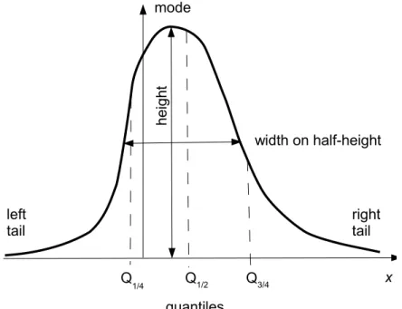
The mode of the distribution is a value of xm at which maximum of p(x) is achieved. If the distribution is monomodal, one can introduce its height as p(xm) and its width on the half-height.
The quantiles of the distribution Qq are the points where RQq
−∞p(x)dx = q. Shown are the lower and the upper quartiles (Q1/4 and Q3/4) and the median,Q1/2.
Figure 1: A sketch of a typical PDF with its mode and tails, and with its robust characteristics.
• The random variables are called (statistically) independent if p(x) can be represented in the form p(x1, x2, ..., xn) = p1(x1)p2(x2)...pn(xn), i.e. factorizes into a product of functions depending on these variables separately. It is necessary to note that statistical independence does not mean anything more than this: the variables still may possess a kind of causal connection.
• The mean of a function of such variables isf(x) = R
f(x)p(x)dx.
• If allp1(x) = p2(x) =...=pn(x) the variablesx1, ..., xnare called independent and identically distributed (iid).
The most important mean is given by the tautology p(y) = R
δ(y−x)p(x)dx, i.e.
p(y) = hδ(y−x)ix.
Notation: If there are more than one variable, and we don’t average over all of them, we list the variables which we average over (i.e. the dumb variables of the corresponding integrations) in the subscript of the angular bracket. The most important consequence of this statement is the formula for the change of variables in the PDF. Let pX(x) be known, and let y=f(x) be the property of interest. If the functionf(x) is invertible, and its inverse is f−1, then
py(y) = Z
δ(y−f(x))px(x)dx =px[f−1(y)]
df−1(y) dy
.
If f is not invertible, but each y admits at most a countable number of roots (i.e. such xi that y=fi(xi)) then
py(y) =X
i
px(fi−1(y))
dfi−1(y) dy
where xi =fi−1(y).
Another important mean is the characteristic function f(k) =heikxi=
Z
eikxp(x)dx.
It does exist (i.e. the integral converges absolutely) for any proper PDF. The characteristic function defines the PDF uniquely (in the same sense as a Fourier-transform identifies the corresponding function).
Note: If the random variable x can only assume non-negative values, the use of the Laplace transform, i.e. calculation of he−uxi gives an alternative tool.
Note that the characteristic function is the generating function of the moments of the distri- bution: Expand the exponential in the Taylor series and obtain
f(k) =
Z X
n
(ikx)n
n! p(x)dx=X
n
(ik)n n!
Z
xnp(x)dx=X
n
(ik)n n! Mn.
The moment Mn is thus (up to a prefactor in) equal to the n-th Taylor coefficient in expansion of f(k) around k = 0. If all moments exist f(k) is analytical function.
Often it is convenient to write
f(k) = heikxix =eψ(k),
i.e. define ψ(k) = lnf(k). The Taylor expansion of ψ(k) gives us the cumulants κn of the distribution:
ψ(k) =
∞
X
n=1
κn
(ik)n n! . The cumulants may be expressed in terms of the moments
κ1 = M1 κ2 = M2−M12
κ3 = M3−3M1M3+ 2M13
κ4 = M4−4M1M3−3M22+ 12M12M2−6M14 ...
Note that the distribution does not have to possess moments or cumulants (i.e. f(k) and ψ(k) are non-analytical) but the corresponding functions f(k) and ψ(k) are still uniquely defined for any distribution.
The same discussion may be made for multivariate distributions (i.e. for the distributions of the vector-valued random variables x= (x1, ..., xn)). The moments are defined as
hxp1xq2...xrni= Z
...
Z
xp1xq2...xrnp(x1, x2, ..., xn)dx1...dxn, and are generated by the characteristic function of the distribution
f(k) = f(k1, ..., kn) =hei(k1x1+k2x2+...+knxn)i
= Z
...
Z
ei(k1x1+k2x2+...+knxn)p(x1, x2, ..., xn)dx1...dxn:
hxp1xq2...xrni= (−i)p+q+...+r∂p+q+...+rf(k)
∂kp1∂k2q...∂knr k=0
.
The logarithm of the characteristic function is the generating function of the cumulants of the distribution.
The change of variables in multivariate distributions is performed analog to the single-variable ones, e.g. ifu=u(x, y) andv =v(x, y), and the inverse transformation exists (i.e. one can express x=x(u, v), y =y(u, v)) then
pu,v(u, v) = px,y(x(u, v), y(u, v))
∂(x, y)
∂(u, v) , and analog for more variables.
If the multivariate (joint) probability distribution is known, the probability density of the results of measurement of each particular variable or of several (but not all) variables may be obtained by calculation the marginal PDF
p(x) = Z
p(x, y)dy
(formally x and y can also be vectors of variables). In many cases we are interested in the distribution of the values of x in experiments giving particular value of y0 as an outcome (i.e.
under the condition that y =y0), e.g. in the conditional probability density p(x|y0) (describing, say, the amount of rain during the days with temperature of 20◦C). By virtue of theBayestheorem
p(x, y) =p(x|y)p(y)
such conditional density is defined when the joint density of x and y is known (note that p(y) is the marginal distribution of y).
1.3 Multivariate Gaussian distributions
Let x = (x1, ..., xn) be the vector of random variables. The multivariate Gaussian probability density function has the form
p(x) =C·exp
−1 2xMx
=C·exp −1 2
n
X
i,j=1
mi,jxixj
! ,
where C is a normalization constant C =
Z ...
Z exp
−1 2xMx
dnx
−1
(which we will explicitly calculate now) and M={mij} is a real, symmetric matrix.
A real symmetric matrix can be diagonalized by an orthogonal coordinate transformationx0 = Ox: M0 =OMO−1 = diag. The matrix O consists of eigenvectors of M taken as rows, and the matrix O−1 =OT consists of the same eigenvectors taken as columns.
Let the (diagonal) elements of M0 be m01, ...m0n. Since the Jacobian of an orthogonal transfor- mation is unity, the integralR
...R
exp(−12xMx)dnxdoesn’t change when passing from xtox0, so
that
C−1 = Z
...
Z
exp(−12xMx)dnx = Z
...
Z
exp(−12x0M0x0)dnx0
= Z
e−12m01x21dx1...
Z
e−12m0nx2ndxn
=
r2π m1...
r2π
mn = (2π)n/2
√
detM0 = (2π)n/2
√
detM. Therefore
p(x) =
√ detM
(2π)n/2 ·exp(−12xMx).
Let us now pay more attention to the meaning of matrix M. Let cij =hxixji=C
Z ...
Z
xixjexp(−12xMx)dnx
be the mean of a product of xi and xj. These means build a matrix C = {cij} (a matrix of covariation coefficients) which is a symmetric and real one. We now note that
cij = C Z
...
Z
xixjexp −1 2
n
X
i,j=1
mijxixj
!
= C·2· ∂
∂mij Z
...
Z
exp −1 2
n
X
i,j=1
mijxixj
!
= 2√ detM (2πn/2)
∂
∂mij
(2π)n/2
√
detM = 1 detM
∂
∂mijdetM.
Let us expand the determinant w.r.t. the column j:
detM=
n
X
i=1
(−1)i+jmijMij, where Mij are the corresponding minors. We now see that
∂
∂mijdetM= (−1)i+jMij, and therefore
cij = (−1)i+jMij
detM =
M−1 ij (7)
i.e. is proportional to the corresponding element of the inverse matrix.
We know well the corresponding relation for a univariate distribution, p(x) = 1
√2πσexp(−x2/2σ2),
when matrix M is essentially a scalar m = 1/σ2 and therefore c=hxxi=σ2 =m−1.
The matrixCalso defines thecharacteristic function of the multivariate Gaussian distribution f(k) = f(k1, ..., kn) = hexp(ikx)i=
Z ...
Z
p(x1, ..., xn)eik1x1+...+iknxn.
We again perform the variable transformationx0 =Ox. Note that the vectorkin the scalar prod- uct is essentially a row-vectorkT, which is transformed by the matrixOT ≡O−1. In the following few lines I will distinguish between the row and the column vectors and write the scalar product explicitly as kTx. We note that the inverse matrix is diagonalized by the same transformation as the initial one, so that (M0)−1 =OM−1O−1, and, respectivelyM−1 =O−1(M0)−1O.
We have:
f(k) =
√detM πn/2
Z ...
Z
exp(−12xTMx) exp(ikTx)dx
=
√detM0 (2π)n/2
Z ...
Z
exp(−12x0TM0x0) exp(ik0Tx0)dx0
=
pQn i=1m0i (2π)n/2
Z ...
Z
exp −12
n
X
i=1
m0i(x0i)2+i
n
X
i=1
ki0x0i
!
dx01...dx0n
=
n
Y
i=1
rm0i 2π
Z
exp −12m0i(x0i)2+ik0ix0i dx0i
=
n
Y
i=1
exp
− 1 2m0i(k0i)2
= exp −1 2
n
X
i=1
(m0i)−1(ki0)2
!
= exp
−1
2k0T(M0)−1k0
= exp
−1
2kTO−1(M0)−1Ok
= exp
−1
2kTM−1k
. This can be rewritten as
f(k) = exp
−1 2kTCk
, and
p(x) = 1
√2πn√
detCexp
−1
2xTC−1x
. These relations will be repeatedly used in what follows.
1.4 Fluctuations of thermodynamical properties
Calculating the second derivatives of the internal energy of the body with respect to all relevant natural variables and using Eq.(5) we obtain a multivariate Gaussian distribution with the matrix M whose elements have no special reason to vanish (end essentially do not vanish anywhere except at the points of phase transitions); the same is true for the elements of the matrixC. As we will see later, these correlations between the changes in different extensive variables indicate the relation between different transport phenomena, for example the non-vanishing correlatorh∆S∆Ni
indicates the connection between heat transport and diffusion. In general, even to obtain the mean value of a fluctuation of a single extensive variable, we have to derive the corresponding matrixM including all relevant extensive variables, invert it to obtain C, and then take the corresponding diagonal element, representing the mean square of fluctuation. There is a way to circumvent this tedious operation.
Let us return to Eq.(4) and note that (∂E/∂V) = −pand (∂E/∂S) =T, so that
∂2E
∂V2∆V + ∂2E
∂V ∂S∆S =−∂p
∂V ∆V − ∂p
∂S∆S ≡ −∆p
∂2E
∂S2∆S+ ∂2E
∂S∂V∆V = +∂T
∂V ∆V +∂T
∂S∆S ≡∆T (8)
where ∆p and ∆T describe the fluctuations of pressure and temperature of the body. Eq.(9) therefore takes the form
p∝exp
−−∆p∆V + ∆T∆S 2kBT0
(9) which is very simple (in the enumerator we see the products of fluctuations of conjugated thermo- dynamic variables), and it is easy to memorize and to generalize, e.g.
p∝exp
−−∆p∆V + ∆T∆S+ ∆µ∆N + ∆σ∆A+...
2kBT0
(10) whereµis the chemical potential, andN the particle’s number,σis the surface tension, andAis the surface area in the system, etc. Moreover, using this equation we can obtain also the fluctuations of intensive variables, or use a mixture of intensive and extensive variables as independent ones.
Imagine, we are interested in the fluctuation of V in a simple fluid body as described by Eq.(9).
Let us consider V and T (and notV and S) as independent observables. Expressing ∆S via ∆T and ∆V we get:
∆S= ∂S
∂T
V
∆T + ∂S
∂V
T
∆V.
The first partial derivative is equal toCV/T, and the second one can be expressed via the Maxwell relation (∂S/∂V)T =∂2F/∂V ∂T =−(∂p/∂T)V. On the other hand,
∆p= ∂p
∂T
V
∆T + ∂p
∂V
T
∆V.
Inserting this in Eq.(9) we get p∝exp
− Cv
2kBT2(∆T)2+ 1 2kBT
∂p
∂V
T
(∆V)2
:
the distribution of an extensive variable factorizes from the one of intensive variables not conjugated to the considered extensive one. Thus:
h(∆V)2i=−kBT ∂V
∂p
T
=kBT V κT, h(∆V∆T)i= 0, h(∆T)2i= kBT2 CV , where κT =−V−1(∂V /∂p) is the isothermic compressibility.
Looking at this example we see that the squared fluctuation of an extensive variable is pro- portional to the volume (mass, number of particles...), and the corresponding r.m.s. fluctuation
to √
V (or √
N). The r.m.s. fluctuations of the densities of extensive variables, and the ones of intensive variables are proportional to 1/√
N or 1/√
V (see however3).
To stress the finding, let us consider p and S as independent variables.
∆V = ∂V
∂p
S
∆p+ ∂V
∂S
p
∆S.
and
∆T = ∂T
∂p
S
∆p+ ∂T
∂S
p
∆S = T
Cp∆S+ ∂T
∂p
S
∆p.
Using the Maxwell relation (∂V /∂S)p =∂2H/∂p∂S = (∂T /∂p)S, we get p∝exp
1 2kBT
∂V
∂p
S
(∆p)2− 1
2kBCp(∆S)2
, so that
h(∆S)2i=kBCp, h(∆S∆p)i= 0, h(∆p)2i=−kBT ∂p
∂V
S
.
The examples above can be generalized and teach us that: If we are interested in the behavior of as single extensive thermodynamical variable, we take all other independent variables to be intensive ones, and the extensive one of interest decouples. If we are interested in the behavior of an intensive thermodynamical variable, we (parallel to what is done previously) take all other independent variables to be extensive ones, and the intensive one of interest decouples. Integrating over these irrelevant variables leaves us with the Gaussian distribution, say, of the form
p(∆V)∝exp
− 1
2kBT V κT
(V −Veq)2
. Comparing this with Eq.(1) we find the corresponding λ = 1/T V κT.
2 Onsager’s Theory of Linear Relaxation Processes
Our discussion will be based on the assumption that the further behavior of the system does not depend on whether the corresponding change in parameters appeared spontaneously as a fluctuation or was introduced on purpose by some preparation procedure. This assumption is called the Onsager’s regression hypothesis (1931). It states that the regression (≈ relaxation) of microscopic thermal fluctuations at equilibrium follows the macroscopic law of relaxation of small non-equilibrium perturbations.
Since statistical physics (whether in equilibrium or not) typically gives us ensemble means of the corresponding properties, we concentrate on such means. Thus we either wait until the measured value of, say, the volume V of a body takes the prescribed value V0 in course of fluctuations and
3 Here we return to our footnote 2, and discuss the restrictions on the possibility to measure these fluctuations of intensive variables. Therefore the deviations of these variables can better be considered as internal parameters of the theory which are linearly connected with the fluctuations of the extensive ones via Eq.(8), and the intensive parameters themselves, defined as means (e.g. in a classical system the temperature as proportional to the mean kinetic energy of the molecules, the pressure as proportional to the mean force acting on the piston, etc.) as non- fluctuating. In any case, when discussing the experimental results for fluctuations of intensive variables, one has to clearly define the measurement operation.
follows then the further evolution ofV(t), or we prepare the body in a state with volume V0 (and other parameters as in the previous experiment) and followV(t). The experiment is repeated many times and we look at the behavior ofhV(t)|V0i, i.e. of theconditional mean of the volume provided the experiment started at a state when this volume was V0. In course of the time hV(t)|V0i will tend to the equilibrium value of the volume V. We thus start from a discussion of relaxation to the equilibrium of the nonequilibrium states introduced on purpose.
2.1 Relaxation to equilibrium
Let us concentrate at the behavior of some macroscopic quantity X characterizing a body of interest, and (at the beginning of our discussion) neglect fluctuations. Let the value of X in equilibrium be X0, and let x = X −X0 (note that X, a natural variable of the entropy, is an extensive variable. Therefore x is also extensive!). Then x = 0 corresponds to equilibrium and x(t) 6= 0 to a nonequilibrium state. The equilibrium state corresponds to a maximum of the entropy of the total system (compound), see Eq.(1). Let us consider the entropy of the system as a function ofx. In equilibrium Sc(x= 0) = max which in a typical case means:
∂Sc
∂x
x=0
= 0;
∂2Sc
∂x2
x=0
≤0.
If a state in whichx6= 0 (which is the state with an entropy which is smaller than the entropy of the equilibrium state) is prepared on purpose and then the system is let to establish the equilibrium, the value of xwill then change approaching zero in order to maximize the entropy. Thus
d
dtSc(x) = ∂Sc
∂x · dx dt ≥0.
We now follow Onsager and give the physical interpretation of the two factors appearing in the last expression.
The derivative
Fx = ∂Sc
∂x
is considered as the driving force of the relaxation to equilibrium. This term is called a thermo- dynamic force (Note that it doesn’t have the dimension of the force, so that the name is not a very proper one! The dimension of the thermodynamic force is [kB][X]−1, i.e. the inverse of the dimension ofX multiplied by Joule per Kelvin), the analogy with mechanics is in the fact that the (negative) entropy plays the role of a “potential energy” which tends to be minimal in equilibrium.
The second term
Jx = dx dt
is called thermodynamic flux or thermodynamic flow of variable x4. Further, Onsager considered situations in which a linear relation between the thermodynamic force and the flux holds:
Jx =LFx,
4The signs in definitions ofF andJ are somewhat arbitrary, and some authors (including myself in some works) define both force and flux with “−”:F =−∂S/∂xandJ =−dx/dt; none of the further relations changes from such an exchange of signs. The difference is whether the entropy or its negative is considered as a corresponding potential.
Taking “+” makes the −S to be more like some mechanical potential energy which is minimal at equilibrium. In the current version of the script I decided to use the “+” the signs.
so that the whole ensuing theory is called linear irreversible thermodynamics. The idea behind is, that the thermodynamic force is the cause of the thermodynamic flow and both should dis- appear at the same time, i.e. when equilibrium is reached. The coefficient L is called Onsager’s phenomenological coefficient, or Onsager’s kinetic coefficient. Since, according the Second Law, the entropy grows when the system approaches equilibrium, the Onsager’s coefficient is strictly positive: Out of equilibrium
0< d
dtS(x) =Jx·Fx =L·Fx2.
The time derivative of the entropy P = dS/dt is called the entropy production, in the Onsager’s linear theory it is a bilinear form
P =J·F
(where we now omit the subscript xindicating the variable). Close to equilibrium F = ∂S
∂X X=X
0+x
= ∂2S
∂x2 x=0
x=−γx.
Using the previous equations we finally get the following linear relaxation dynamics
˙
x=−Lγx.
Introducing
λ=Lγ
being the so-called relaxation coefficient of the quantity xwe get finally
˙
x=−λx. (11)
This linear kinetic equation describes the relaxation of a thermodynamic system prepared in a non-equilibrium state to its equilibrium one. Starting with the initial state x(0) the dynamics of the variable x(t) is then
x(t) =x(0) exp(−λt) =x(0) exp
−t τ
. (12)
where τ = λ−1 is a typical decay time of the initial deviation from equilibrium (the relaxation time).
A similar procedure can be performed when dealing with several thermodynamic variables.
Close to equilibrium the entropy as a function of xi,(i= 1...N) is given by S(x1, ..., xn) =Smax− 1
2 X
i,j
γijxixj
whereγij are given by Eq.(6)withγ introduced in Eq.(2)5. Following the Onsager’s ideas we define the thermodynamic forces
Fi =−X
j
γijxj and fluxes
Ji = ˙xi.
5The matrixγ is connected with the matrixMdescribing fluctuations viaγij =kBmij.
The generalized linear Onsager-Ansatz now reads Ji =X
j
LijFj
(note that the flux of a variableiis caused also by forces corresponding to other variables, remember the Le-Chatelier principle for indirect changes). The Second Law again requires the positivity of the entropy production, and thus
Lijxixj ≥0,
where the equality takes place only for xi = 0, (i= 1, ..., n). This corresponds to the requirement of positive definiteness of the matrix Lij. Parallel to above,
˙
xi =X
j
LijFj
and introducing the matrix of relaxation coefficients of the linear processes near equilibrium states we end up with
˙
xi =−X
j
λijxj (13)
with
λij =X
k
Likγkj
(i.e. in the matrix formλ=Lγ). Since the matrix γij determines the dispersion of the stationary fluctuations close to equilibrium, we see that there exists an intimate relation between fluctuations and relaxation, i.e. we have a fluctuation-dissipation relation for a set of fluctuating and relaxing variables6.
In the next chapter we will discuss the phenomenological equations of linear nonequilibrium thermodynamics (Fourier equation for heat transport, Ficks equation for diffusion, other, more complex cases), but first return to our fluctuations, and discuss what do we learn about the properties of the kinetic coefficients from what we know about them.
Although our discussion was conducted for thermodynamic variables (i.e. for a small subsystem being a fluid body), it can be generalized to a broader class of relaxation phenomena. Let us consider an example of a (macroscopic) harmonic oscillator in the contact with the bath. Eq.(3) p∝ exp(−R/kBT) gives the connection of the probability of fluctuation with the reversible work necessary to create the state of the subsystem observed. For an oscillator it is
R= ∆E = kx2 2 + p2
2m = kx2
2 + mv2 2
(in this equation x is the coordinate of the center of mass, and p is the momentum, not the probability). Therefore the joint probability density to find the position x and the velocity v is
p(v, x)∝exp
− kx2
2kBT − mv2 2kBT
,
6The matrixLof kinetic coefficients is, of course, real and positively defined, but does not have to be symmetric, as we will see later. Therefore the matrixλdoes not have to be symmetric as well. Its eigenvalues may be complex (although the physical fact that the system always relaxes to equilibrium suggests that the real parts of these eigenvalues are positive). Therefore in the case when the system has to be described by more than one extensive variable, the relaxation processes may be oscillatory.
i.e. is given by the Gibbs-Boltzmann distribution. The entropy reads S(x, v) = kBlnW =const− kx2
2T − mv2 2T . Therefore the elements of the matrix γ are:
γ11 = k
T, γ22= m
T , γ12=γ21 = 0.
The vector of thermodynamical forces has then the components Fx = ∂S
∂x =−kx T = f
T where f is the mechanical force, and
Fp = ∂S
∂p =−v
T =− p mT.
The fact that according to the upper equation the thermodynamical force is proportional to the mechanical force was the reason why I use the non-standard sign convention. Using pinstead of v is not important in this equation, but it is pthat in a large system that is an extensive variable!
Let us now put down the Onsager’s equations for the thermodynamical flux J= ( ˙x,p).˙
˙
x = L11
−kx T
+L12
−v T
˙
p = L21
−kx T
+L22
−v T
In the case of vanishing friction we compare this with the Hamiltonian equations of motion:
˙
x = p m =v
˙
p = −kx and get
L11 =L22 = 0, L12 =−T, L21=T.
Note the relation L12 =−L21, which is a special case of the Onsager-Casimir relation which will be discussed later. In the case with friction, when the equation of motion of the damped oscillator reads m¨x=−γx˙ −kxwe get
L11= 0, L22=γT, L12=−T, L21 =T.
We see therefore that these mechanical cases fall into the general Onsager’s scheme of linear relaxation processes.
2.2 Relaxation of fluctuations
It is interesting to know, what kind of a random process can describe the fluctuations of some properties of interest x(t) as a function of time7, i.e. what is their temporal dynamics. Since our system is at equilibrium (none of its relevant properties changes with time), the properties of the fluctuations do not depend on when the observation started, and the corresponding random process isstationary. This means for example that all properties of the process x(t) at two different times (e.g. the correlation functions hx(t1)x(t2)i) depend only on the difference of the times, i.e. time lag τ =t2−t1, and not on t1 and t2 separately.
If fluctuations can be neglected, it is reasonable to assume that
˙
xi =−X
j
λijxj,
and (as we will discuss) experiments in many cases support this assumption. The fluctuations can be neglected if (a) the body is so large that the fluctuations are small and/or (b) the deviation from the equilibrium x(t) is much larger that the fluctuation background h(∆x)2i1/2. It is reasonable to assume that when the value of x(t) gets smaller than the correlation background, the time evolution of theensemble mean of x(t) is still well-described by Eq.(11) or Eq.(13), i.e. in the last case
hx˙i(t)i=−X
j
λijhxj(t)i.
Here again the experiments show that the assumption is quite reasonable in a vast amount of cases.
In the case of the system prepared on purpose the means are the ones under given initial condi- tions, and in the case of fluctuations they are the conditional means hx˙i(t)|x(0)i and hxj(t)|x(0)i.
Experiments show that similar equations hold not only for thermodynamical variables, but for a larger class of variables (e.g. for macroscopic velocities or momenta of bodies in the contact with bath); special cases will be considered later.
Let us consider the correlation functions
Cij(t1, t2) =hxi(t1)xj(t2)i.
Since the process of fluctuations close to equilibrium is stationary, Cij(t1, t2) can only depend on the time lag τ = t2 −t1: Cij(t1, t2) = Cij(t2 −t1) ≡ Cij(τ). On the same reason t1 can always be set to zero. Note that the matrix C discussed in §1.2 is a matrix of single-time correlations cij =Cij(0). For a stationary process we have
Cij(τ) = hxi(0)xj(τ)i=hxi(t)xj(t+τ)i
= hxj(t+τ)xi(t)i=hxj(t0)xi(t0−τ)i=Cji(−τ).
(in the fourth expression I interchanged the sequence of multipliers; t0 =t+τ).
Since hxj(t)|x(0)i decays according to adeterministic system of linear differential equations d
dthxj(t)|x(0)i=−X
i
λjihxi(t)|x(0)i,
7i.e. what are the properties of the collection of the values of the corresponding observable at different timest
we can multiply both sides this equation byxj(0), and then average over the equilibrium distribu- tion of all x(0) to get the corresponding unconditional mean:
hxi(0)d
dthxj(t)|x(0)iix(0) =−X
i
λjkhxi(0)hxk(t)|x(0)iix(0)
or d
dthxi(0)xj(t)i=−X
k
λjkhxi(0)xk(t)i (Bayes theorem!), i.e.
d
dtCij(t) = −X
k
λjkCik(t).
There exists a very important relation between the fluctuations of thermodynamical variables xi and the corresponding forces Fi (which we will often denote by Xi in what follows: a capital letter denotes a force, the small letter denotes the variable). The distribution of x is a Gaussian
p(x)∝exp(−12xTMx),
with M = k−1B γ, so that hxixji = Cij(0) = (M−1)ij. On the other hand, the vector of ther- modynamical forces F (or X) is X = −γx = −kBMx. We note that the square, symmetric matrix M is invertible (all eigenvalues are positively defined, no infinite fluctuations), we can write x=−(1/kB)M−1X. The Jacobian of this transformation is constant (∝detM) and thus
p(X)∝exp(−12kB−2XTM−1MM−1X) = exp(−12kB−2XTM−1X).
Therefore hXiXji=kB2mij. Let us now use Xi =−kBP
kmikxk and calculate hXixji = −hkBX
k
mikxkxji=−kBX
k
mikhxkxji=−kBX
k
mikckj
= −kBX
k
(M)ik(M−1)kj =−kB(MM−1)ij =−kBδij (where in the last line the expression Eq.(7) is used).
We note that in the case whenxi corresponds to the deviation from equilibrium of an extensive thermodynamical variable this result reproduces the decoupling of this extensive variable from deviations of non-conjugated intensive ones in the Einstein’s theory of fluctuations.
2.3 Microscopic reversibility and symmetry of kinetic coefficients
Changingτ to−τ means the reversal of the “direction of time”, which in the microscopic language corresponds to the reversal of all momenta, electric currents and therefore magnetic fields, etc.
Let us now consider what happens with macroscopic variables x. The variables which are the functions of coordinates only, and for those which are the quadratic functions of momenta (like the kinetic or total energy, and therefore for the internal energy as well) stay the same under this transformation:
xi(t) =xi(−t).
Such variables are called even variables. On the other hand, the variables depending linearly on the momenta or currents (total momentum, magnetization, etc) change their sign,
xi(t) =−xi(−t),
and are called odd variables. This behavior is a consequence of the principle of microscopic reversibility of motion. The property of being even or odd will be called the parity of the corresponding variable: it is equal to i = 1 for the even variable and i = −1 for the odd one.
Therefore
Cij(τ) =hxi(t)xj(t+τ)i=±hxi(−t)xj(−t−τ)i=±Cij(−τ)
depending on whether the parity of the of the both variables is the same or different: if it is the same, the sign is “+”, and when it is different, the sign is “−”, i.e.
Cij(τ) =ijCij(−τ).
We now use this notation and put down d
dτxi(τ) = X
k
LikXk(τ) d
dτxj(τ) = X
k
LjkXk(τ).
We multiply the first equation with xj(0), the second equation with xi(0), and average over the realizations:
d
dτhxi(τ)xj(0)i = X
k
LikhXk(τ)xj(0)i d
dτhxj(τ)xi(0)i = X
k
LjkhXk(τ)xi(0)i.
The l.h.s. of the corresponding equations are the time derivatives of Cij(−τ) = Cji(τ) and of Cji(−τ) =jiCji(τ), so that
d
dτCji(τ) = X
k
LikhXk(τ)xj(0)i ij d
dτCji(τ) = X
k
LjkhXk(τ)xi(0)i.
Now we go to the limit τ →0+ and use that hXixji=−kBδij: C˙ji(τ)
τ→0+ =kB
X
k
Likδkj =−kBLij
ij C˙ji(τ)
τ→0+ =kBX
k
Ljkδki =−kBLji. From this we get that
Lij =ijLji. (14)
Equation Eq.(14) gives us the famousOnsager-Casimirrelation defining the symmetry of kinetic coefficients.
2.4 Simple examples
While discussing the size of fluctuations of thermodynamical variables we relied on the isothermal situation of a body or other smaller system in a contact with a heat bath, the existence of the bath was never assumed when considering the kinetic coefficients and symmetry thereof. We only used the fact that at equilibrium the entropy of the isolated composite system reaches its maximum.
Therefore we can consider the situation with several (two or more) subsystems of comparable size building together an isolated system. We suppose that each of them can be characterized by a set of thermodynamical parameters (the assumption of local equilibrium).
2.4.1 Example 1: Heat transport
Let us consider two subsystems forming a composit isolated one. At the beginning of the experi- ment they are separated by an adiabatic wall and have different temperatures T1 and T2. At time t = 0 the adiabatic wall is replaced by a weakly heat conducting one. At each instant of time each of the systems will be considered as being at local equilibrium at some temperatureT1(t) and T2(t).
T1 T2 → T1(t) T2(t) adiabatic wall dE1 =−dE2 (no heat transport) heat conduction During the equilibration
0< dS = ∂S1(E1, ...)
∂E1 dE1+∂S2(E2, ...)
∂E2 dE2
= 1
T1dE1+ 1 T2dE2
= 1
T1 − 1 T2
dE1 :
The heat flows from the warmer to the colder subsystem, which leads to the equilibration of temperature. The thermodynamic force corresponding to the variable E1 is F =T2−1−T1−1. The phenomenological linear Ansatz than implies
Q˙ ≡E˙1 =J = dE1
dt =L( 1 T1 − 1
T2)' L
T2(T2−T1) = ˜L(T2−T1) (J – the heat flux,L – the empirical kinetic coefficient,T =√
T1T2 is a (geometric) mean temper- ature of the reservoirs). Taking dQ =C1dT1 = −C2dT2, (C1, C2 – the specific heat values of the subsystems) we get
dT1 dt =
L˜
C1(T2−T1) dT2
dt = −L˜
C2(T2−T1).
We note that this system of equations has an integral of motion, the total energy C1T1+C2T2 = const, so that it can be easily solved by substitution. We get
T1 = [T1(0)−T¯] exp −L˜ C˜t
! + ¯T T2 = [T2(0)−T¯] exp −L˜
C˜t
! + ¯T with
C˜ = C1C2 C1+C2 and
T¯= C1T1(0) +C2T2(0) C1+C2
being the final temperatures of the subsystems. The temperatures relax exponentially to their final values.
2.4.2 Example 2: Mass transport
N1 N2 → N1(t) N2(t) impenetrable wall dN1 =−dN2 (no mass transport) porous wall
We consider the transport of particles between the two containers of the volumes V1 and V2 (the concentrations are proportional to the corresponding numbers of particles, and the coefficient of this proportionality is the volume). The particles considered are either in an ideal solution (or in a gas phase) so that the chemical potentials are equal to µ1,2 =const+RTlnn1,2, and
S =S0 −R(N1lnn1+N2lnn2).
The total number of particles stays constant: V1n1+V2n2 =N. Therefore dS
dt =−RT[V1n˙1lnn1+V1n˙1+V2n˙2lnn2+V2n˙2] =RT V1n˙1[lnn2−lnn1] (since V2n˙2 =−V1n˙1). The particle flux close to equilibrium is
J = ˙n1 =LRT V1(lnn2−lnn1)'L(n˜ 2−n1).
Note that the situation considered here is much more the equilibration of concentrations due to the (osmotic) pressure difference than the true diffusion. True diffusion takes place under equal total pressure in both containers and assumes that another component (solvent) is diffusing in the opposite direction.