Profr. Dr. Wolf-Tilo Balke
Institut für Informationssysteme
Technische Universität Braunschweig http://www.ifis.cs.tu-bs.de
Distributed Data Management
3.0 Query Processing
3.1 Basic Distributed Query Processing 3.2 Data Localization
3.3 Response Time Models
3.0 Introduction
• There a 3 major architectures for DDBMS
– Share-Everything Architecture
• Nodes share main memory
• Suitably for tightly coupled high performance highly parallel DDBMS
• Weaknesses wrt. scalability and reliability
– Shared-Disk Architecture
• Nodes have access to same secondary storage (usually SAN)
• Strengths w.r.t. complex data and transactions
• Common in enterprise level DDBMS
– Share-Nothing Architecture
• Node share nothing and only communicate over network
• Common for web-age DDBMS and the cloud
• Strength w.r.t. scalability and elasticity
Architectures
• Data has to be distributed across nodes
• Main concepts:
– Fragmentation: partition all data into smaller fragments / “chunks”
• How to fragment? How big should fragments be? What should fragments contain?
– Allocation: where should fragments be stored?
• Distribution and replication
• Where to put which fragment? Should fragments be replicated? If yes, how often and where?
Fragmentation
• In general, fragmentation and allocation are optimization problem which are closely depended on the actual application
– Focus on high availability?
– Focus on high degree of distribution?
– Focus on low communication costs and locality?
– Minimize or maximize geographic diversity?
– How complex is the data?
– Which queries are used how often?
• Many possibilities and decisions!
Fragmentation
• The task of DB query processing is to answer user queries
– e.g. “How many students are at TU BS in 2016?”
• Answer: 20 037
• However, some additional constraints must be satisfied
– Low response times – High query throughput – Efficient hardware usage – …
– Relational Databases 2!
3.0 Query Processing
• The generic workflow for centralized query processing involves multiple steps and
components
3.0 Query Processing
Parser Query
Rewriter
Query Optimizer
Physical Optimizer
Query Execution
Query Result
Query Pre-Processing Data Meta Data
• Query, Parser, and Naïve Query Plan
– Usually, the query is given by some higher-degree declarative query language
• Most commonly, this is SQL
– The query is translated by parser into some internal representation
• Called naïve query plan
• This plan is usually described by an relational algebra operator tree
3.0 Query Processing
Query
• Example:
– Database storing mythical creatures and heroes
• Creature(cid, cname, type); Hero(hid, hname)
• Fights(cid, hid, location, duration)
– “Return the name of all creatures which fought at the Gates of Acheron”
• SELECT cname FROM creature c, fights f WHERE c.cid=f.cid
AND location=“Gates Of Acheron”
3.0 Query Processing
• Example (cont.)
– Translate to relational algebra
• 𝜋𝑐𝑛𝑎𝑚𝑒𝜎𝑙𝑜𝑐𝑎𝑡𝑖𝑜𝑛=′𝐺𝑜𝐴′∧𝑐𝑟𝑒𝑎𝑡𝑢𝑟𝑒.𝑐𝑖𝑑=𝑓𝑖𝑔ℎ𝑡𝑠.𝑐𝑖𝑑𝑐𝑟𝑒𝑎𝑡𝑢𝑟𝑒 × 𝑓𝑖𝑔ℎ𝑡𝑠
• In contrast to the SQL statement, the algebra statement already contains the required basic evaluation operators
3.0 Query Processing
• Example (cont.)
– Represent as operator tree
3.0 Query Processing
𝜋𝑐𝑛𝑎𝑚𝑒
𝜎𝑙𝑜𝑐𝑎𝑡𝑖𝑜𝑛=′𝐺𝑜𝐴′∧ 𝑐𝑟𝑒𝑎𝑡𝑢𝑟𝑒.𝑐𝑖𝑑=𝑓𝑖𝑔ℎ𝑡𝑠.𝑐𝑖𝑑
×
𝐶𝑟𝑒𝑎𝑡𝑢𝑟𝑒𝑠 𝐹𝑖𝑔ℎ𝑡𝑠
• After the naïve query plan is found, the query rewriter performs simple transformations
– Simple optimizations which are always beneficial regardless of the system state (Algebraic Query Rewriting)
• Mostly, cleanup operations are performed
• Elimination of redundant predicates
• Simplification of expressions
• Normalization
• Unnesting of subqueries and views
• etc.
– System state
• Size of tables
• Existence or type of indexes
• Speed of physical operations
• etc.
3.0 Query Processing
Query Rewriter
Meta Data
• The most effort in query preprocessing is spent on query optimization
– Algebraic Optimization
• Find a better relational algebra operation tree
• Heuristic query optimization
• Cost-based query optimization
• Statistical query optimization
– Physical Optimization
• Find suitable algorithms for implementing
the operations
3.0 Query Processing
Query Optimizer
Physical Optimizer
• Heuristic query optimization
– Use simple heuristics which usually lead to better performance
– Basic Credo: Not the optimal plan is needed, but the really crappy plans have to be avoided!
– Heuristics
• Break Selections
– Complex selection criteria should be broken into multiple parts
• Push Projection and Push Selection
– Cheap selections and projections should be performed as early as possible to reduce intermediate result size
• Force Joins
– In most cases, using a join is much cheaper than using a Cartesian product and a selection
3.0 Query Processing
• Example (cont.)
– Perform algebraic optimization heuristics
• Push selection & Projection
• Force Join
3.0 Query Processing
𝜋𝑐𝑛𝑎𝑚𝑒
𝜎𝑙𝑜𝑐𝑎𝑡𝑖𝑜𝑛=′𝐺𝑜𝐴′
⋈
𝐶𝑟𝑒𝑎𝑡𝑢𝑟𝑒𝑠
𝐹𝑖𝑔ℎ𝑡𝑠
𝜋𝑐𝑖𝑑, 𝑐𝑛𝑎𝑚𝑒 𝜋𝑐𝑖𝑑
• Most non-distributed RDBMS rely strongly on cost- based optimizations
– Aim for better optimized plan which respect system and data characteristics
• Especially, join order optimization is a challenging problem
– Idea
• Establish a cost model for various operations
• Enumerate all query plans
• Pick best query plan
– Usually, dynamic programming techniques are used to keep computational effort manageable
3.0 Query Processing
• Algebraic optimization results in an optimized query plan which is still represented by
relational algebra
– How is this plan finally executed?
• > Physical Optimization
– There are multiple algorithms for implementing a given relational algebra operation
• Join: Block-Nested-Loop join? Hash-join? Merge-Join? etc.
• Select: Scan? Index-lookup? Ad-hoc index generation &
lookup? etc.
• …
3.0 Query Processing
• Physical optimization translates the query plan into an execution plan
– Which algorithms will be used on which data and indexes?
• Physical Relational Algebra
– For each standard algebra operation, several physical implementations are offered
• Should pipelining (iterator model) be used? How?
– Physical and algebraic optimization are often tightly interleaved
• Most physical optimization also relies on cost-models
• Idea: perform cost-based optimization algorithm “in one sweep”
for algebraic, join order, and physical optimization
3.0 Query Processing
• Example (cont.)
3.0 Query Processing
Filter all but cname
Index Key Lookup:
fights.location=“GoA”
Index Nested Loop Join
Table 𝐶𝑟𝑒𝑎𝑡𝑢𝑟𝑒𝑠 Primary Index
Of Creatures
• In general, centralized non-distributed query processing is a well understood problem
– Current problems
• Designing effective and efficient cost models
• Eliciting meaningful statistics for use in cost models
• Allow for database self-tuning
3.0 Query Processing
• Distributed query processing (DQP) shares many properties of centralized query processing
– Basically, the same problem…
– But: objectives and constraints are different!
• Objectives for centralized query processing
– Minimize number of disk accesses!
– Minimize computational time
3.1 Basic DQP
• Objectives for distributed query processing are usually less clear…
– Minimize resource consumption?
– Minimize response time?
– Maximize throughput?
• Additionally, costs are more difficult to predict
– Hard to elicit meaningful statistics on network and remote node properties
• Also, high variance in costs
3.1 Basic DQP
• Additional cost factors, constraints, and problems must be respected
– Extension of physical relational algebra
• Sending and receiving data
– Data localization problems
• Which node holds the required data?
– Deal with replication and caching – Network models
– Response-time models
– Data and structural heterogeneity
• Think federated database…
3.1 Basic DQP
• Often, static enumeration optimizations are difficult in distributed setting
– More difficult than non-distributed optimization
• More and conflicting optimization goals
• Unpredictability of costs
• More costs factors and constraints
• Quality-of-Service agreements (QoS)
– Thus, most successful queries optimization techniques are adaptive
• Query is optimized on-the-fly using current, directly measured information of the system’s behavior and workload
– Don’t target for the best plan, but for a good plan
3.1 Basic DQP
• Example distributed query processing:
– “Find the creatures involved in fights being decided in exactly one minute”
• 𝜋𝑐𝑛𝑎𝑚𝑒𝜎𝑑𝑢𝑟𝑎𝑡𝑖𝑜𝑛=1𝑚𝑖𝑛𝑐𝑟𝑒𝑎𝑡𝑢𝑟𝑒 ⋈ 𝑓𝑖𝑔ℎ𝑡𝑠
– Problem:
• Relations are fragmented and distributed across five nodes
• The creature relation uses primary horizontal partitioning by creature type
– One fragment of the relation is located at node 1, the other on node 2;
no replication
• The fights relation uses derived horizontal partitioning
– One fragment on node 3, one on node 4; no replication
• Query originates from node 5
3.1 Basic DQP
3.1 Basic DQP
N1
N2 N3
N4 N5
𝐶𝑟𝑒𝑎𝑡𝑢𝑟𝑒𝑠1
𝐶𝑟𝑒𝑎𝑡𝑢𝑟𝑒𝑠2 𝐹𝑖𝑔ℎ𝑡𝑠1
𝐹𝑖𝑔ℎ𝑡𝑠2 Query
• Cost model and relation statistics
– Accessing a tuple (tupacc) costs 1 unit
– Transferring a tuple (tuptrans) costs 10 units – There are 400 creatures and 1000 fights
• 20 fights are one minute
• All tuples are uniformly distributed
– i.e. node 3 and 4 contain 10 short-fight-tuples each
– There are local indexes on attribute “duration”
• Direct tuple access possible on a local sites, no scanning
– All nodes may directly communicate with each other
3.1 Basic DQP
3.1 Basic DQP
N1
N2 N3
N4 N5
𝐶𝑟𝑒𝑎𝑡𝑢𝑟𝑒𝑠1
𝐶𝑟𝑒𝑎𝑡𝑢𝑟𝑒𝑠 𝐹𝑖𝑔ℎ𝑡𝑠1
𝐹𝑖𝑔ℎ𝑡𝑠2 Query
𝜋𝑐𝑛𝑎𝑚𝑒𝜎𝑑𝑢𝑟𝑎𝑡𝑖𝑜𝑛=1𝑚𝑖𝑛𝑐𝑟𝑒𝑎𝑡𝑢𝑟𝑒 ⋈ 𝑓𝑖𝑔ℎ𝑡𝑠
200 tuples
200 tuples 500 tuples
10 matches
500 tuples 10 matches
• Two simple distributed query plans
– Version A: Transfer all data to node 5
3.1 Basic DQP
𝜋𝑐𝑛𝑎𝑚𝑒 (𝐶𝑟𝑒𝑎𝑡𝑢𝑟𝑒1 ∪ 𝐶𝑟𝑒𝑎𝑡𝑢𝑟𝑒2) ⋈ (𝜎𝑑𝑢𝑟𝑎𝑡𝑖𝑜𝑛=1𝑚𝑖𝑛𝐹𝑖𝑔ℎ𝑡𝑠1 ∪ 𝐹𝑖𝑔ℎ𝑡𝑠2) Node 5
Receive 𝐶𝑟𝑒𝑎𝑡𝑢𝑟𝑒1 Receive 𝐶𝑟𝑒𝑎𝑡𝑢𝑟𝑒1 Receive 𝐹𝑖𝑔ℎ𝑡𝑠1 Receive 𝐹𝑖𝑔ℎ𝑡𝑠2
Send 𝐶𝑟𝑒𝑎𝑡𝑢𝑟𝑒1
Node 1
Send 𝐶𝑟𝑒𝑎𝑡𝑢𝑟𝑒2
Node 2 Node 4
Send 𝐹𝑖𝑔ℎ𝑡𝑠2
Node 3
Send 𝐹𝑖𝑔ℎ𝑡𝑠1
– Version B: ship intermediate results
3.1 Basic DQP
𝜋𝑐𝑛𝑎𝑚𝑒 (𝐶𝑟𝑒𝑎𝑡𝑢𝑟𝑒1∗ ∪ 𝐶𝑟𝑒𝑎𝑡𝑢𝑟𝑒2∗) Node 5
𝐶𝑟𝑒𝑎𝑡𝑢𝑟𝑒1∗
Receive𝐹𝑖𝑔ℎ𝑡𝑠1∗ Send 𝐹𝑖𝑔ℎ𝑡𝑠1∗
Node 3 𝐶𝑟𝑒𝑎𝑡𝑢𝑟𝑒1⋈𝐹𝑖𝑔ℎ𝑡𝑠1
∗
Node 1
Send 𝐶𝑟𝑒𝑎𝑡𝑢𝑟𝑒1∗
Receive𝐹𝑖𝑔ℎ𝑡𝑠2∗ Send 𝐹𝑖𝑔ℎ𝑡𝑠2∗
Node 4
𝐶𝑟𝑒𝑎𝑡𝑢𝑟𝑒2⋈𝐹𝑖𝑔ℎ𝑡𝑠2∗
Node 2
Send 𝐶𝑟𝑒𝑎𝑡𝑢𝑟𝑒2∗ 𝐶𝑟𝑒𝑎𝑡𝑢𝑟𝑒2∗
• Costs A: 23.000 Units
3.1 Basic DQP
𝜋𝑐𝑛𝑎𝑚𝑒 (𝐶𝑟𝑒𝑎𝑡𝑢𝑟𝑒1 ∪ 𝐶𝑟𝑒𝑎𝑡𝑢𝑟𝑒2) ⋈ (𝜎𝑑𝑢𝑟𝑎𝑡𝑖𝑜𝑛=1𝑚𝑖𝑛𝐹𝑖𝑔ℎ𝑡𝑠1 ∪ 𝐹𝑖𝑔ℎ𝑡𝑠2) Node 5
Receive 𝐶𝑟𝑒𝑎𝑡𝑢𝑟𝑒1 Receive 𝐶𝑟𝑒𝑎𝑡𝑢𝑟𝑒1 Receive 𝐹𝑖𝑔ℎ𝑡𝑠1 Receive 𝐹𝑖𝑔ℎ𝑡𝑠2
Send 𝐶𝑟𝑒𝑎𝑡𝑢𝑟𝑒1
Node 1
Send 𝐶𝑟𝑒𝑎𝑡𝑢𝑟𝑒2
Node 2 Node 4
Send 𝐹𝑖𝑔ℎ𝑡𝑠2
Node 3
Send 𝐹𝑖𝑔ℎ𝑡𝑠1 200*tuptrans
=2.000
200*tuptrans
=2.000
500*tuptrans
=5.000
500*tuptrans
=5.000
1.000*tupacc
=1.000
(selection w/o index)
400*20*tupacc
=8.000 (BNL join)
tupacc=1; tuptrans=10
• Cost B: 460 Units
3.1 Basic DQP
𝜋𝑐𝑛𝑎𝑚𝑒 (𝐶𝑟𝑒𝑎𝑡𝑢𝑟𝑒1∗ ∪ 𝐶𝑟𝑒𝑎𝑡𝑢𝑟𝑒2∗) Node 5
𝐶𝑟𝑒𝑎𝑡𝑢𝑟𝑒1∗
Receive𝐹𝑖𝑔ℎ𝑡𝑠1∗ Send 𝐹𝑖𝑔ℎ𝑡𝑠1∗
Node 3 𝐶𝑟𝑒𝑎𝑡𝑢𝑟𝑒1⋈𝐹𝑖𝑔ℎ𝑡𝑠1
∗
Node 1
Send 𝐶𝑟𝑒𝑎𝑡𝑢𝑟𝑒1∗
Receive𝐹𝑖𝑔ℎ𝑡𝑠2∗ Send 𝐹𝑖𝑔ℎ𝑡𝑠2∗
Node 4
𝐶𝑟𝑒𝑎𝑡𝑢𝑟𝑒2⋈𝐹𝑖𝑔ℎ𝑡𝑠2∗
Node 2
Send 𝐶𝑟𝑒𝑎𝑡𝑢𝑟𝑒2∗ 𝐶𝑟𝑒𝑎𝑡𝑢𝑟𝑒2∗
10*tuptrans
=100
10*tuptrans
=100
20*tupacc
=20
20*tupacc
=20
10*tuptrans
=100
10*tuptrans
=100 tupacc=1; tuptrans=10
• For performing any query optimization meta data is necessary
– Meta data is stored in the catalog
– The catalog of a DDBMS especially has to store information on data distribution
• Typical catalog contents
– Database schema
• Definitions of tables, views, UDFs & UDTs, constraints, keys,
etc.
3.1 Basic DQP
– Partitioning schema
• Information on how the schema is partitioned and how tables can be reconstructed
– Allocation schema
• Information on where which fragment can be found
• Thus, also contains information on replication of fragments
– Network information
• Information on node connections
• Connection information (network model)
– Additional physical information
• Information on indexes, data statistics (basic statistics, histograms,
3.1 Basic DQP
• Central problem in DDBMS:
Where and how should the catalog be stored?
– Simple solution: store at a central node
– For slow networks, it beneficial to replicate the catalog across many / all nodes
• Assumption: catalog is small and does not change often
– Also, caching is a viable solution
• Replicate only needed parts of a central catalog, anticipate potential inconsistencies
– In rare cases, the catalog may grow very large and may change often
• Catalog has to be fragmented and allocated
• New meta problem: where to find which catalog fragment?
3.1 Basic DQP
• What should be optimized when and where?
– We assume that most applications use canned queries
• i.e. prepared and parameterized SQL statements
• Full compile time-optimization
– Similar to centralized DBs, the full query execution plan is computed at compile time
– Pro:
• Queries can be directly executed
– Con:
• Complex to model
• Many information unknown or too expensive to gather (collect statistics on all nodes?)
• Statistics outdated
3.1 Basic DQP
• Fully dynamic optimization
– Every query is optimized individually at runtime – Heavily relies on heuristics, learning algorithms, and
luck – Pro
• Might produce very good plans
• Uses current network state
• Also usable for ad-hoc queries
– Con
• Might be very unpredictable
• Complex algorithms and heuristics
3.1 Basic DQP
• Semi-dynamic and hierarchical approaches
– Most DDBMS optimizers use semi-dynamic or hierarchical optimization techniques (or both) – Semi-dynamic
• Pre-optimize the query
• During query execution, test if execution follows the plan
– e.g. if tuples/fragments are delivered in time, if network has predicted properties, etc.
• If execution shows severe plan deviations, compute a new query plan for all missing parts
3.1 Basic DQP
• Hierarchical Approaches
– Plans are created in multiple stages – Global-Local Plans
• Global query optimizer creates a global query plan
– i.e. focus on data transfer: which intermediate results are to be computed by which node, how should intermediate results be shipped, etc.
• Local query optimizers create local query plans
– Decide on query plan layout, algorithms, indexes, etc. to deliver the requested intermediate result
3.1 Basic DQP
– Two-Step-Plans
• During compile time, only stable parts of the plan are computed
– Join order, join methods, access paths, etc.
• During query execution, all missing plan elements are added
– Node selection, transfer policies, …
• Both steps can be performed using traditional query optimization techniques
– Plan enumeration with dynamic programming
– Complexity is manageable as each optimization problem is much easier than a full optimization
3.1 Basic DQP
• The first problem in distributed query processing is data localization
– Problem: query transparency is needed
• User queries the global schema
• However, the relations of global schema are fragmented and distributed
– Assumption
• Fragmentation is given by partitioning rules
– Selection predicates for horizontal partitioning – Attribute projection for vertical partitioning
• Each fragment is allocated only at one node
– No replication
• Fragmentation rules and location of the fragments is stored in catalog
3.2 Data Localization
• Base Idea:
– Query Rewriter is modified such that each query to global schema is replaced by a query on the
distributed schema
• i.e. each reference to a global relation is replaced by a localization program which reconstructs the table
– If the localization program reconstructs the full relation, this is called a generic query
– Often, the full relation is not necessary and by
inspecting the query, simplifications can be performed
3.2 Data Localization
• Example:
– Relation 𝐶𝑟𝑒𝑎𝑡𝑢𝑟𝑒 = (𝑐𝑖𝑑, 𝑐𝑛𝑎𝑚𝑒, 𝑡𝑦𝑝𝑒) – Primary partitioning by id
• 𝐶𝑟𝑡1 = 𝜎𝑐𝑖𝑑≤100𝐶𝑟𝑒𝑎𝑡𝑢𝑟𝑒
• 𝐶𝑟𝑡2 = 𝜎100<𝑐𝑖𝑑<200𝐶𝑟𝑒𝑎𝑡𝑢𝑟𝑒
• 𝐶𝑟𝑡3 = 𝜎𝑐𝑖𝑑≥200𝐶𝑟𝑒𝑎𝑡𝑢𝑟𝑒
– Allocate each fragment to its own node
• 𝐶𝑟𝑡1 to node 1, …
– A generic localization program for 𝐶𝑟𝑒𝑎𝑡𝑢𝑟𝑒 is given by
• 𝐶𝑟𝑒𝑎𝑡𝑢𝑟𝑒 = 𝐶𝑟𝑡 ∪ 𝐶𝑟𝑡 ∪ 𝐶𝑟𝑡
3.2 Data Localization
• Global queries can now easily be transformed to generic queries by replacing table references
– SELECT * FROM creatures WHERE cid = 9
• Send and receive operations are implicitly assumed
3.2 Data Localization
𝜎𝑐𝑖𝑑=9
𝐶𝑟𝑒𝑎𝑡𝑢𝑟𝑒𝑠 Global Query
∪
𝐶𝑟𝑡1 𝐶𝑟𝑡2 𝐶𝑟𝑡3
Localization P. for Creatures
𝜎𝑐𝑖𝑑=9
∪
𝐶𝑟𝑡1 𝐶𝑟𝑡2 𝐶𝑟𝑡3 Generic Query
• Often, when using generic queries, unnecessary fragments are transferred and accessed
– We know the partitioning rules, so it is clear that the requested tuple is in fragment 𝐶𝑟𝑡1
– Use this knowledge to reduce the query
3.2 Data Localization
𝜎𝑐𝑖𝑑=9
𝐶𝑟𝑡1
Reduced Query
• In general, the reduction rule for primary horizontal partitioning can be stated as
– Given fragments of 𝑅 as 𝐹𝑅 = 𝑅1, … , 𝑅𝑛 with 𝑅𝑗 = 𝜎𝑃𝑗(𝑅)
– Reduction Rule 1:
• All fragments 𝑹𝒋 for which 𝝈𝒑𝒔 𝑹𝒋 = ∅ can be omitted from localization program
– 𝒑𝒔 is the query selection predicate
– e.g. in previous example, 𝑐𝑖𝑑 = 9 contradicts 100 < 𝑐𝑖𝑑 < 200
• 𝜎𝑝𝑠 𝑅𝑗 = ∅ ⇐ ∀𝑥 ∈ 𝑅: ¬(𝑝𝑠 𝑥 ∧ 𝑝𝑗(𝑥))
• “The selection with the query predicate 𝑝𝑠 on the fragment 𝑅𝑗 will be empty if 𝑝𝑠 contradicts the partitioning predicate 𝑝𝑗 of 𝑅𝑗”
3.2 Data Localization
• Join Reductions
– Similar reductions can be performed with queries involving a join and relations partitioned along the join attributes
– Base Idea: Larger joins are replaced by multiple partial joins of fragments
• 𝑹𝟏 ∪ 𝑹𝟐 ⋈ 𝑺 ≡ 𝑹𝟏 ⋈ 𝑺 ∪ (𝑹𝟐 ⋈ 𝑺)
• Which might or might not be a good idea depending on the data or system
• Reduction: Eliminate all those unioned fragments from evaluation which will return an empty result
3.2 Data Localization
• i.e.: join according to the join graph
– Join graph usually not known (full join graph assumed)
• Discovering the non-empty partial joins will construct join graph
3.2 Data Localization
Fragments of R Fragments of S
R 1R 2R 34 S1 S2 S3 S
• We hope for
– …many partial joins which will definitely produce empty results and may be omitted
• This is not true if partitioning conditions are suboptimal
– …many joins on small relations have lower resource costs than one large join
• Also only true if “sensible” partitioning conditions used
• Not always true, depends on used join algorithm and data distributions; still a good heuristic
– …smaller joins may be executed in parallel
• Again, this is also not always a good thing
• May potentially decrease response time…
– Response time cost models!
• …but may also increase communication costs
3.2 Data Localization
• Example:
– 𝐶𝑟𝑒𝑎𝑡𝑢𝑟𝑒 = (𝑐𝑖𝑑, 𝑐𝑛𝑎𝑚𝑒, 𝑡𝑦𝑝𝑒)
• 𝐶𝑟𝑡1 = 𝜎𝑐𝑖𝑑≤100𝐶𝑟𝑒𝑎𝑡𝑢𝑟𝑒
• 𝐶𝑟𝑡2 = 𝜎100<𝑐𝑖𝑑<200𝐶𝑟𝑒𝑎𝑡𝑢𝑟𝑒
• 𝐶𝑟𝑡3 = 𝜎𝑐𝑖𝑑≥200𝐶𝑟𝑒𝑎𝑡𝑢𝑟𝑒
– 𝐹𝑖𝑔ℎ𝑡𝑠 = (𝑐𝑖𝑑, ℎ𝑖𝑑, 𝑙𝑜𝑐𝑎𝑡𝑖𝑜𝑛, 𝑑𝑢𝑟𝑎𝑡𝑖𝑜𝑛)
• 𝐹𝑔1 = 𝜎𝑐𝑖𝑑≤200𝐹𝑖𝑔ℎ𝑡𝑠
• 𝐹𝑔2 = 𝜎𝑐𝑖𝑑>200𝐹𝑖𝑔ℎ𝑡𝑠
– SELECT * FROM creature c, fight f WHERE c.cid=f.cid
3.2 Data Localization
3.2 Data Localization
⋈
𝐶𝑟𝑒𝑎𝑡𝑢𝑟𝑒𝑠
Global Query
𝐹𝑖𝑔ℎ𝑡𝑠
⋈
𝐶𝑟𝑡1
Generic Query
∪
𝐶𝑟𝑡2 𝐶𝑟𝑡3 𝐹𝑔1
∪
𝐹𝑔2
∪
𝐶𝑟𝑡1
Reduced Query
⋈
𝐹𝑔1 𝐶𝑟𝑡2
⋈
𝐶𝑟𝑡3
⋈
𝐹𝑔2
• By splitting the joins, six fragment joins are created
• 3 of those fragment joins are empty
• e.g. 𝐶𝑟𝑡1 ⋈ 𝐹𝑔2 = ∅
• 𝐶𝑟𝑡1contains tuples with cid≤100
• 𝐹𝑔2 contains tuples with cid>200
• Formally
– Join Fragmentation
• 𝑅1 ∪ 𝑅2 ⋈ 𝑆 ≡ 𝑅1 ⋈ 𝑆 ∪ (𝑅2 ⋈ 𝑆)
– Reduction Rule 2:
𝑅𝑖 ⋈ 𝑅𝑗 = ∅ ⇐ ∀𝑥 ∈ 𝑅𝑖, 𝑦 ∈ 𝑅𝑗: ¬(𝑝𝑖 𝑥 ∧ 𝑝𝑗(𝑦))
• “The join of the fragments 𝑅𝑗 and 𝑅𝑖 will be empty if their respective partition predicates (on the join attribute)
contradict.”
– i.e. there is no tuple combination 𝑥 and 𝑦 such that both partitioning predicates are fulfilled at the same time
• Empty join fragments may be reduced
3.2 Data Localization
• Obviously, the easiest join reduction case follows from derived horizontal fragmentation
– For each fragment of the first relation, there is
exactly one matching fragment of the second relation
• The reduced query will always be more beneficial than the generic query due to small number of fragment joins
– Derived horizontal fragmentation is especially effective to represent one-to-many relationships
• Many-to-many relationships are only possible if tuples are replicated
– No fragment disjointness!
3.2 Data Localization
• Example:
– 𝐶𝑟𝑒𝑎𝑡𝑢𝑟𝑒 = (𝑐𝑖𝑑, 𝑐𝑛𝑎𝑚𝑒, 𝑡𝑦𝑝𝑒)
• 𝐶𝑟𝑡1 = 𝜎𝑐𝑖𝑑≤100𝐶𝑟𝑒𝑎𝑡𝑢𝑟𝑒
• …
– 𝐹𝑖𝑔ℎ𝑡𝑠 = (𝑐𝑖𝑑, ℎ𝑖𝑑, 𝑙𝑜𝑐𝑎𝑡𝑖𝑜𝑛, 𝑑𝑢𝑟𝑎𝑡𝑖𝑜𝑛)
• 𝐹𝑔1 = 𝐹𝑖𝑔ℎ𝑡𝑠 ⋉ 𝐶𝑟𝑒𝑎𝑡𝑢𝑟𝑒
• …
– SELECT * FROM creature c, fight f WHERE c.cid=f.cid
3.2 Data Localization
∪
𝐶𝑟𝑡1
Reduced Query
⋈
𝐹𝑔1 𝐶𝑟𝑡2
⋈ 𝐶𝑟𝑡3
⋈
𝐹𝑔2 𝐹𝑔3
• Reduction for vertical fragmentation is very similar
– Localization program for 𝑅 is usually of the form
• 𝑅 = 𝑅1 ⋈ 𝑅2
– When reducing generic vertically fragmented queries, avoid joining in fragments containing useless attributes – Example:
• 𝐶𝑟𝑒𝑎𝑡𝑢𝑟𝑒 = (𝑐𝑖𝑑, 𝑐𝑛𝑎𝑚𝑒, 𝑡𝑦𝑝𝑒) is fragmented to
𝐶𝑟𝑒𝑎𝑡𝑢𝑟𝑒1 = (𝑐𝑖𝑑, 𝑐𝑛𝑎𝑚𝑒) and 𝐶𝑟𝑒𝑎𝑡𝑢𝑟𝑒2 = (𝑐𝑖𝑑, 𝑡𝑦𝑝𝑒)
• For the query SELECT cname FROM creature WHERE cid=9, no access to 𝐶𝑟𝑒𝑎𝑡𝑢𝑟𝑒2 is necessary
3.2 Data Localization
• Reducing Queries w. Hybrid Fragmentation
– Localization program for 𝑅 combines joins and unions
• e.g. 𝑅 = (𝑅1∪ 𝑅2) ⋈ 𝑅3
– General guidelines are
• Remove empty relations generated by contradicting selections on horizontal fragments
– Relations containing useless tuples
• Remove useless relations generated by vertical fragments
– Relations containing unused attributes
• Break and distribute joins, eliminate empty fragment joins
– Fragment joins with guaranteed empty results
3.2 Data Localization
• Previously, we computed reduced queries from global queries
• However, where should the query be executed?
– Assumption: only two nodes involved
• i.e. client-server setting
• Server stores data, query originates on client
– Query shipping
• Common approach for centralized DBMS
• Send query to the server node
• Server computes the query result and ships result back
3.2 Data Localization
– Data Shipping
• Query remains at the client
• Server ships all required data to the client
• Client computes result
3.2 Data Localization
Server Client
σ
⋈ receive
Query Shipping Data Shipping
Client
⋈
Server σ
σ σ
send
receive receive
send send
• Hybrid Shipping
– Partially send query to server – Execute some query parts at the server, send intermediate results to client
– Execute remaining query at the client
3.2 Data Localization
Hybrid Shipping Client
⋈
Server
receive receive
send send
σ σ
• Of course, these simple models can be extended to multiple nodes
– Query optimizer has to decide which parts of the query have to be shipped to which node
• Cost model!
– In heavily replicated scenarios, clever hybrid shipping can effectively be used for load balancing
• Move expensive computations to lightly loaded nodes
• Avoid expensive communications
3.2 Data Localization
• “Classic” DB cost models focus on
total resource consumption of a query
– Leads to good results for heavy computational load and slow network connections
• If query saves resources, many queries can be executed in parallel on different machines
– However, queries can also be optimized for short response times
• “Waste” some resources to get query results earlier
• Take advantage of lightly loaded machines and fast connections
• Utilize intra-query parallelism
– Parallelize one query instead of multiple queries
3.3 Response Time Models
• Response time models are needed!
– “When does the first result tuple arrive?”
– “When have all tuples arrived?”
• Example
– Assume relations or fragments A, B, C, and D – All relations/fragments are available on all nodes
• Full replication
– Compute 𝐴 ⋈ 𝐵 ⋈ 𝐶 ⋈ 𝐷 – Assumptions
• Each join costs 20 time units (TU)
• Transferring an intermediate result costs 10 TU
• Accessing relations is free
3.3 Response Time Models
• Two plans:
– Plan 1: Execute all operations on one node
• Total costs: 60
– Plan 2: Join on different nodes, ship results
• Total costs: 80
3.3 Response Time Models
Node 1
A
⋈ ⋈
⋈
B C D
Node 1
A
⋈ ⋈
B C D
Send Send
Node 2 Node 3
Receive Receive
⋈
Plan 1
Plan 2
• With respect to total costs, plan 1 is better
• Example (cont.)
– But: Plan 2 is better wrt. to response time as operations can be carried out in parallel
3.3 Response Time Models
Plan 2
Plan 1 𝐴 ⋈ 𝐵 𝐶 ⋈ 𝐷
𝐴𝐵 ⋈ 𝐶𝐷 𝐶 ⋈ 𝐷 𝑇𝑋
𝑇𝑋
𝐴𝐵 ⋈ 𝐶𝐷
𝐴 ⋈ 𝐵
• Response Time
– Two types of response times
• First Tuple & Full Result Response Time
• Computing response times
– Sequential execution parts
• Full response time is sum of all computation times of all used operations
– Multiple parallel threads
• Maximal costs of all parallel sequences
3.3 Response Time Models
• Considerations:
– How much speedup is possible due to parallelism?
• Or: “Does kill-it-with-iron” work for parallel problems?
– Performance speed-up of algorithms is limited by Amdahl’s Law
• Gene Amdahl, 1968
• Algorithms are composed of parallel and sequential parts
• Sequential code fragments severely limit potential
speedup of parallelism!
3.3 Response Time Models
– Possible maximal speed-up:
• 𝑚𝑎𝑥𝑠𝑝𝑒𝑒𝑑𝑢𝑝 ≤ 𝑝
1+𝑠∗ 𝑝−1
• 𝑝 is number of parallel threads
• 𝑠 is percentage of single-threaded code
– e.g. if 10% of an algorithm is sequential, the
maximum speed up regardless of parallelism is 10x
– For maximal efficient parallel systems, all sequential bottlenecks have to be identified and eliminated!
3.3 Response Time Models
3.3 Response Time Models
• Good First Tuple Response benefits from queries executed in a pipelined fashion
– Not pipelined:
• Each operation is fully completed and a intermediate result is created
• Next operation reads intermediate result and is then fully completed
– Reading and writing of intermediate results costs resources!
– Pipelined
• Operations do not create intermediate results
• Each finished tuple is fed directly into the next operation
• Tuples “flow” through the operations
3.3 Response Time Models
• Usually, the tuple flow is controlled by iterator interfaces implemented by each operation
– “Next tuple” command
– If execution speed of operations in the pipeline
differ, tuples are either cached or the pipeline blocks
• Some operations are more suitable than others for pipelining
– Good: scan, select, project, union, … – Tricky: join, intersect, …
– Very Hard: sort
3.3 Response Time Models
• Simple pipeline example:
– Tablescan, Selection, Projection
• 1000 tuples are scanned, selectivity is 0.1
– Costs:
• Accessing one tuple during tablescan: 2 TU (time unit)
• Selecting (testing) one tuple: 1 TU
• Projecting one tuple: 1 TU
3.3 Response Time Models
FInal
Projection
IR1 IR2
Selection Selection
Projection
Pipeline
Final
time event
2 First tuple in IR1 2000 All tuples in IR1 2001 First tuple in IR2 3000 All tuples in IR2 3001 First tuple in Final
time event
2 First tuple finished tablescan
3 First tuple finished selection (if
selected…)
4 First tuple in Final 3098 Last tuple finished
tablescan
3099 Last tuple finished selection
Pipelined Non-Pipelined
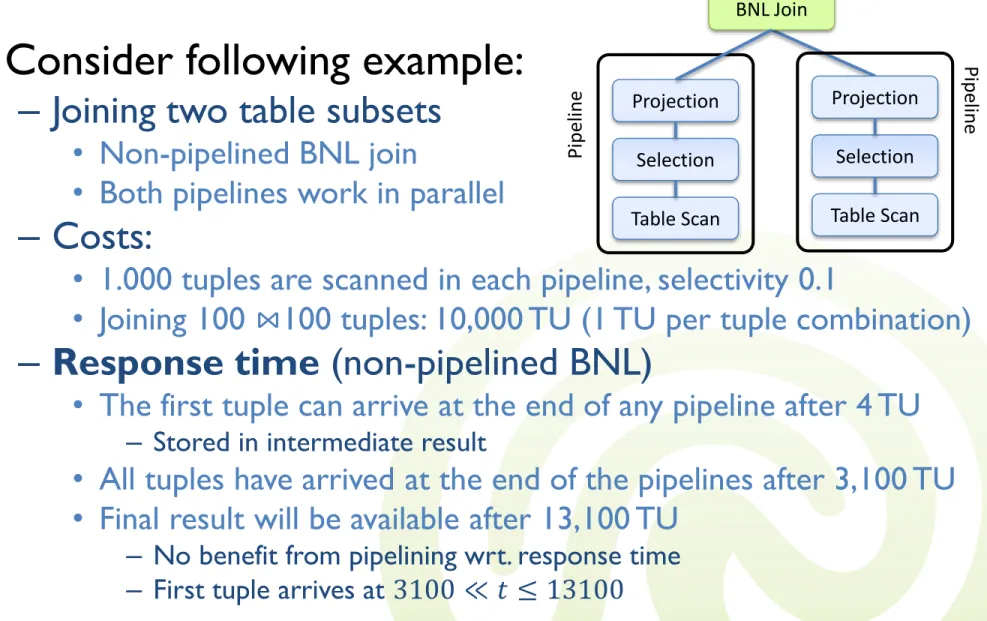
• Consider following example:
– Joining two table subsets
• Non-pipelined BNL join
• Both pipelines work in parallel
– Costs:
• 1.000 tuples are scanned in each pipeline, selectivity 0.1
• Joining 100 ⋈100 tuples: 10,000 TU (1 TU per tuple combination)
– Response time (non-pipelined BNL)
• The first tuple can arrive at the end of any pipeline after 4 TU
– Stored in intermediate result
• All tuples have arrived at the end of the pipelines after 3,100 TU
• Final result will be available after 13,100 TU
– No benefit from pipelining wrt. response time – First tuple arrives at 3100 ≪ 𝑡 ≤ 13100
3.3 Response Time Models
Table Scan Selection Projection
Table Scan Selection Projection
BNL Join
Pipeline
Pipeline
• The suboptimal result of the previous example is due to the unpipelined join
– Most traditional join algorithms are unsuitable for pipelining
• Pipelining is not usually necessary feature in a strict single thread environment
– Join is fed by two input pipelines
– Only one pipeline can be executed at a time
– Thus, at least one intermediate result has to be created – Join may be performed single / semi-pipelined
• In parallel / distributed DBs, fully pipelined joins are beneficial
3.3 Response Time Models
• Single-Pipelined-Hash-Join
– One of the “classic” join algorithms – Base idea 𝑨 ⋈ 𝑩
• One input relation is read from an intermediate result (B), the other is pipelined though the join operation (A)
• All tuples of B are stored in a hash table
– Hash function is used on the join attribute
– i.e. all tuples showing the same value for the join attribute are in one bucket
» Careful: hash collisions! Tuple with different joint attribute value might end up in the same bucket!
• Every incoming tuple a (via pipeline) of A is hashed by join attributed
• Compare a to each tuple in the respective B bucket
– Return those tuples which show matching join attributes
3.3 Response Time Models
• Double-Pipelined-Hash-Join
– Dynamically build a hashtable for A and B each
• Memory intensive!
– Process tuples on arrival
• Cache tuples if necessary
• Balance between A and B tuples for better performance
• Rely on statistics for a good A:B ratio
– If a new A tuple a arrives
• Insert a into the A-table
• Check in the B table if there are join partners for a
• If yes, return all matching AB tuples
– If a new B tuple arrives, process it analogously
3.3 Response Time Models
Hash Tuple 17 A1, A2
31 A3
Hash Tuple
29 B1
A B
A Hash B Hash
Input Feeds AB
Output Feed
𝑨 ⋈ 𝑩
31 B2
3.3 Response Time Models
Hash Tuple 17 A1, A2
31 A3
Hash Tuple
29 B1
31 B2
A B
A Hash B Hash
AB
Output Feed
𝑨 ⋈ 𝑩
31 B2
• B(31,B2) arrives
• Insert into B Hash
• Find matching A tuples
• Find A3
• Assume that A3 matches B2…
• Put AB(A3, B2) into output feed
• In pipelines, tuples just “flow” through the operations
– No problem with that in one processing unit…
– But how do tuples flow to other nodes?
• Sending each tuple individually may be very ineffective
– Communication costs:
• Setting up transfer & opening communication channel
• Composing message
• Transmitting message: header information & payload
– Most protocols impose a minimum message size & larger headers – Tuplesize ≪ Minimal Message Size
• Receiving & decoding message
• Closing channel
3.3 Response Time Models
• Idea: Minimize Communication Overhead by Tuple Blocking
– Do not send single tuples, but larger blocks containing multiple tuples
• “Burst-Transmission”
• Pipeline-Iterators have to be able to cache packets
• Block size should be at least the packet size of the underlying network protocol
– Often, larger packets are more beneficial – ….more cost factors for the model
3.3 Response Time Models
• Additional constraints and cost factors compared to “classic” query optimization
– Network costs, network model, shipping policies – Fragmentation & allocation schemes
– Different optimization goals
• Response time vs. resource consumption
• Basic techniques try to prune unnecessary accesses
– Generic query reductions
Distributed Query Processing
• This lecture only covers very basic techniques
– In general, distributed query processing is a very complex problem
– Many and new optimization algorithms are researched
• Adaptive and learning optimization
• Eddies for dynamic join processing
• Fully dynamic optimization
• …
• Recommended literature
– Donald Kossmann: “The state of the Art in Distributed Query Processing”, ACM Computing Surveys, Dec. 2000
Distributed Query Processing
• Distributed Transaction Management
– Transaction Synchronization
– Distributed Two-Phase Commits – Byzantine Agreements