Working Paper
Using Genome Graph Topology to Guide Annotation Matrix Sparsification
Author(s):
Danciu, Daniel; Karasikov, Mikhail; Mustafa, Harun; Kahles, André; Rätsch, Gunnar Publication Date:
2020-11-19 Permanent Link:
https://doi.org/10.3929/ethz-b-000464846
Originally published in:
bioRxiv , http://doi.org/10.1101/2020.11.17.386649
Rights / License:
Creative Commons Attribution-NonCommercial 4.0 International
This page was generated automatically upon download from the ETH Zurich Research Collection. For more information please consult the Terms of use.
Using Genome Graph Topology to Guide Annotation Matrix Sparsification
Daniel Danciu1,2,* Mikhail Karasikov1,2,3,∗ Harun Mustafa1,2,3 Andr´e Kahles1,2,3,† Gunnar R¨atsch1,2,3,4,†
1Biomedical Informatics Group, Department of Computer Science, ETH Zurich, Zurich, Switzerland
2Biomedical Informatics Research, University Hospital Zurich, Zurich, Switzerland
3Swiss Institute of Bioinformatics, Zurich, Switzerland
4Department of Biology, ETH Zurich, Zurich, Switzerland
Abstract
Since the amount of published biological sequencing data is growing exponentially, efficient methods for storing and indexing this data are more needed than ever to truly benefit from this invaluable resource for biomedical research. Labeled de Bruijn graphs are a frequently-used approach for representing large sets of sequencing data. While significant progress has been made to succinctly represent the graph itself, efficient methods for storing labels on such graphs are still rapidly evolving. In this paper, we present RowDiff, a new technique for compacting graph labels by leveraging expected similarities in annotations of nodes adjacent in the graph. RowDiff can be constructed in linear time relative to the number of nodes and labels in the graph, and the construction can be efficiently parallelized and distributed, significantly reducing construction time. RowDiff can be viewed as an intermediary sparsification step of the initial annotation matrix and can thus naturally be combined with existing generic schemes for compressed binary matrix representation. Our experiments on the Fungi subset of the RefSeq collection show that applying RowDiff sparsification reduces the size of individual annotation columns stored as compressed bit vectors by an average factor of 42. When combining RowDiff with a Multi-BRWT representation, the resulting annotation is 26 times smaller than Mantis-MST, the previously known smallest annotation representation. In addition, experiments on 10,000 RNA-seq datasets show that RowDiff combined with Multi-BRWT results in a 30% reduction in annotation footprint over Mantis-MST.
1 Introduction
The exponential increase in global sequencing capacity [1] and the resulting growth of public sequence repositories have created an urgent need for the development of compact representation schemes of bio- logical sequences. Such schemes should not only maintain all relevant biological sequence variation but also provide fast access for sequence search and extraction. After initial attempts focused on the lossless compression of full sequences, e.g., using the Burrows-Wheeler transform [2], the field soon turned towards representing a proxy of the input sequences instead: the sets of allk-mers contained in them. For this, any recurrent occurrence of a substring of length k in the input is represented by a uniquek-mer, forming a k-mer set. A query of a given sequence against the input text can then be replaced by exactk-mer matching against the set. Longer strings are queried as a succession ofk-mers. Although it is a lossy representation of the input (as, e.g., repeats longer thankare collapsed), constructingk-mer sets has proved highly useful in practice [3, 4, 5, 6].
*Joint-first authors.
†Joint corresponding authors; contact: andre.kahles@inf.ethz.ch and gunnar.ratsch@ratschlab.org.
1.1 Representation ofk-mer sets
Various representations have been developed to balance the trade-off between the space taken by thek-mer set and query time or representation accuracy. Conceptually, thek-mer set fully defines a node-centricde Bruijngraph, where eachk-mer forms a node and edges are represented implicitly, based on whether any two nodes share a k−1 overlap. The simplest representations are bitmaps or (perfect) hash-tables that indicate the presence or absence of any possiblek-mer over the input alphabet in the input text. While non- optimal in space, they offer constant-time query ofk-mers. More compact representations use approximate membership query data structures to probabilistically represent a de Bruijn graph [7, 8] or utilize succinct de Bruijn graphs (a generalization of the Burrows-Wheeler transform) [9], which usually require less than one byte per inputk-mer over the nucleotide alphabet{A, C, G, T}.
1.2 De Bruijn graph annotation
A major limitation of the above representations is that the identities of any sequence labels contained in the input text set are lost. To alleviate this, the concept ofcolored de Bruijn graphsemerged [10], allowing for the representation of additional annotations perk-mer. These annotations can either be stored in conjunction with thek-mers or be organized in a separate data structure, using thek-mer representation only as an index space. Although the first option is used by a number of conceptually interesting methods, such as Mantis [11]
that uses counting quotient filters to represent thek-mers linked to an annotation identifier, here we will only focus on the second option, as it allows for the connection of arbitrary annotations to thek-mer set, without re-processing thek-mer index.
Conceptually, the set of annotations is a relation between k-mers and labels that can be represented as a binary matrix, where the k-mer set indexes the rows and each annotation label specifies a column.
Any entry(i, j) in the matrix represents the relation ofk-meriand annotationj. Different methods have been suggested to compress this annotation matrix in a way that still allows for efficient query. VARI [12]
concatenates the rows of the annotation matrix and compresses the result using either an RRR [13] or Elias- Fano coding [14, 15]. Rainbowfish [16] takes advantage of high redundancy in matrix rows by computing a frequency code for the unique rows, compressing the unique rows in a matrix ordered by these codes, then representing the original matrix as a variable-length code vector. However, this method and other frequency coding-based approaches become less effective for data sets with greater levels of noise or inter-sample variability. Multi-BRWT [17] compresses the matrix in a hierarchical tree structure exploiting column similarity, but leaving the possible row redundancy unexploited. All of these methods share the common property that they act as general purpose binary matrix compressors, and thus, they do not take into account any particular domain knowledge in their construction.
1.3 Leveraging graph topology to improve annotation compression
While the methods mentioned above rely solely on similarities between annotation matrix elements to achieve their compression, a few have additionally leveraged graph topology to increase their compression potential. The Bloom filter correction method introduced by [18] encodes the columns of the annotation matrix in Bloom filters with high false positive rate. Assuming that all nodes within a graph unitig share identical annotations, a row in the annotation matrix (corresponding to all nodes from the same unitig in the graph) is computed as the bit-wise AND of the rows stored for every node of that unitig.
The more recently introduced Mantis MST method [19] constructs an annotation graph with nodes representing the unique rows of the annotation matrix. In this annotation graph, a weighted edge between two nodes v1 andv2 is created if there exist adjacent nodes s1 ands2 in the underlying de Bruijn graph whose annotations are represented byv1andv2, respectively. The weight of this edge(v1, v2)is then set to the Hamming distance of the unique rowsv1 andv2. Mantis MST computes the minimal spanning tree of
the annotation graph and represents the annotation of a node as its bit-wise XOR with the annotation of its parent node in the spanning tree, while only the annotation of the root node is represented explicitly.
1.4 Our contribution
We present a new scheme for representing graph annotations, RowDiff, which takes advantage of simi- larities between the annotations of neighboring nodes to compress annotation matrices. RowDiff can be constructed in linear time relative to the input size and has a small memory footprint, thus making it suitable for annotating virtually arbitrarily large graphs. Since RowDiff is a transformation of the input annotation matrix attempting to increase its sparsity, RowDiff can be naturally chained with any generic scheme for compressed binary matrix representation to achieve further improvements in compression performance.
In the next sections, we define the underlying concepts (Sections 2.1 and 2.2) and detail our methods for construction (Sections 2.3 to 2.4) and querying (Section 2.5) of the RowDiff data structures. We then describe the test datasets (Section 3.1) and study the construction time (Section 3.2) and representation sizes (Sections 3.3 and 3.4) of RowDiff-compressed annotations. Finally, we discuss limitations and directions for future work (Section 4).
2 Method
2.1 Idea Sketch
RowDiff relies on the observation that neighboring nodes in the de Bruijn graph are likely similarly anno- tated, which implies that storing differences between rows corresponding to adjacentk-mers may be more space efficient than storing the full rows.
We propose the RowDiff transform that converts an annotation matrix of a de Bruijn graph into a new annotation matrix of the same size and an anchor bit vector. The anchor vector stores which rows remain unchanged. We show that the original annotation matrix can be reconstructed from the RowDiff trans- formed matrix (and the anchor vector). Empirically, the RowDiff transformed matrix is significantly better compressible in the typical case where neighboring nodes have similar annotations. We develop an efficient algorithm for defining good anchors and for computing the RowDiff transform (and inverse).
2.2 RowDiff transformation
For each node in the de Bruijn graph we arbitrarily define its RowDiff successor as its lexicographically largest adjacentk-mer. We will use the terms node and row interchangeably to denote both a node in the de Bruijn graph and its corresponding annotation row.
RowDiff replaces each row with the (likely sparser) delta relative to its RowDiff successor. For binary rows, the delta is simply the element-wise XOR relative to the successor, while for non-binary rows, the delta could store the difference between the row and its successor. In order to be able to reconstruct the original annotation, some rows are left unchanged. A node for which the annotation is stored unchanged is called ananchor. Nodes with zero out-degree (calledsinks) do not have a RowDiff successor, and must thus be anchors.
RowDiff defines a transformation of the original annotation matrix to a RowDiff-transformed matrix.
Algorithm 1 shows the implementation of theinverse transformation, which reconstructs the original row from the RowDiff representation.
Algorithm 1Row annotation reconstruction
1: functionRECONSTRUCTANNOTATION(node) 2: row←get row(node)
3: whilenodeis not an anchordo 4: node←Successor(node)
5: row←row⊕get row(node) .⊕: bit-wise XOR
6: end while 7: returnrow 8: end function
Starting from any node in the de Bruijn graph, Algorithm 1 defines a traversal leading to an anchor node for which the annotation was not transformed. get row(node)returns the sparsified row for the given node or the original annotation row, if this node is an anchor. Since de Bruijn graphs may have cycles, additional anchor nodes might have to be assigned in order to break RowDiff cycles (those cycles where every node is a RowDiff successor relative to its predecessor in the cycle).
Proposition 1. Algorithm 1 finishes for every starting node, and therefore, reconstructs the original anno- tation, if and only if every sink node in the graph is an anchor and every RowDiff cycle has at least one anchor node in it.
Once the set of anchor nodes satisfies Proposition 1, the RowDiff-transformed matrix together with the anchor vector of the anchor nodes set encode the original annotation matrix.
2.3 Anchor assignment
In addition to the small set of anchors described in Proposition 1, we assign more nodes as anchors to limit the length of each RowDiff path traversed in order to reconstruct a node annotation and thereby ensuring that Algorithm 1’s time complexity is bounded by a constant. We cap the maximum RowDiff path length to a certain valueM (typically between 10 to 100) by making everyM-th node in a RowDiff path an anchor.
At the same time, since anchor nodes require storing the original, less sparse annotation row, it is desirable to minimize the total number of anchor nodes in order to keep the annotation size small.
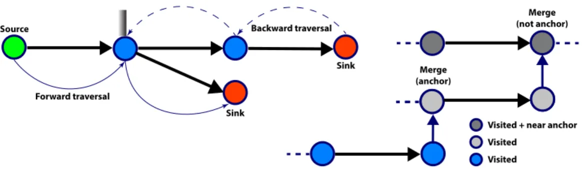
The following anchor assignment algorithm allocates anchor nodes near-optimally in three steps as follows (see Algorithm 2). First, we traverse backwards (in parallel) starting with sink nodes, i.e. nodes with zero out-degree (see Algorithm S1). The traversal of a path stops at a bifurcation if the current node is not the last outgoing for its source node (Figure 1, left). When the length of the current path reaches a multiple ofM, the current node is marked as an anchor node. Once the backward traversal is finished, the vast majority of the nodes have been traversed, and anchor allocation is optimal, in the sense that no anchors are closer thanM to each other. In the second step, we start with source nodes, i.e. nodes with in-degree zero, and traverse RowDiff paths forward, by always selecting the last outgoing edge at a bifurcation (see Algorithm S2). Traversal stops when we reach an already visited node. Lastly, in the third step, we start traversing forward at all forks with unvisited nodes.
One important detail in the forward traversal step is handling the situation when the traversal stops due to merging into a visited node. Not doing anything may result in arbitrarily long paths with no anchors (when such merges are chained). Always setting an anchor at a merge will introduce unnecessary anchors and increase the annotation size. We handle merges with the following simple heuristic: use an additional bit vector,nearAnchor, to mark all nodes that are known to be at a distance smaller thanM to an anchor node. When hitting a merge during forward traversal, we only set an anchor node if the merge node is not marked innearAnchor, i.e. we have a chained merge (Figure 1, right). An optimal algorithm for deciding if a merge node should create an anchor would require labeling each node with the distance to its nearest anchor. In our implementation we preferred the heuristic algorithm due to its significantly reduced memory footprint.
Forward traversal
Backward traversal Source
Sink
Sink
Merge (not anchor)
Merge (anchor)
Visited
Visited + near anchor Visited
Figure 1: Left: RowDiff traversal. When traversing forward, the last outgoing edge is selected. When traversing backward to assign anchor nodes, the traversal stops when reaching an edge that is not the last outgoing edge of its source node.Right:Chained merge. Grey nodes represent traversed nodes, darker grey arenearAnchor. When traversing the light grey nodes, we merge into anearAnchor, so no anchor is set. When traversing the blue nodes, an anchor must be set at the merge, as the node is not marked asnearAnchor
Algorithm 2Anchor assignment
1: functionASSIGNANCHORS(M)
2: visited[]← {False} .initialize mask of visited nodes
3: anchor[]← {False} .initialize mask of anchor nodes
4: for alls∈Sinks()parallel do
5: anchor←TraverseBwd(s, visited, anchor,M) 6: for alls∈Sources()parallel do
7: anchor←TraverseFwd(s, visited, anchor,M) 8: for alls∈Forks()parallel do
9: anchor←TraverseFwd(s, visited, anchor,M) 10: for alls∈Nodes()parallel do
11: anchor←TraverseFwd(s, visited, anchor,M) 12: returnanchor
13: end function
Another anchor setting strategy would be to generate unitigs and mark all nodes at the end of a unitig as an anchor. This strategy, which is equivalent to setting an anchor at all bifurcations and merges, lead to an 80% increase in annotation size (relative to a diff annotation with infinite maximum path lengthM) when tested on microbial genomes. While the penalty in annotation size is significant, the quick construction time and faster query time may make this option attractive for certain applications.
2.3.1 Anchor optimization
To guarantee that none of the rows in RowDiff has more set bits than the corresponding row in the original annotation, which may happen when two adjacent nodes carry completely different annotations, we perform an anchor optimization procedure on RowDiff. For each node in the graph, we compute the difference between the number of set bits in its original row and the RowDiff-transformed one. Then, each node with a negative difference is made an anchor. This ensures that all rows in the RowDiff-transformed annotation matrix are at least as sparse as the corresponding rows in the original annotation matrix.
Proposition 2. Each row in a RowDiff-transformed annotation matrix has the same or smaller number of set bits than its corresponding row in the original annotation matrix.
The anchor optimization procedure is implemented similarly to the initial construction of RowDiff (see Section 2.4), thus it has the same time and memory complexity.
2.4 RowDiff construction
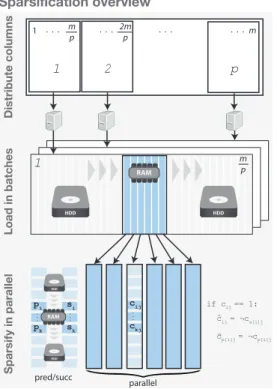
The sparsification workflow is schematically described inFigure 2. The initial sparsification of annotation columns can be trivially parallelized by dividing the columns into groups and processing each group on
a different machine. Each machine processes columns in batches. The size of each batch is determined dynamically by loading columns into memory until a desired upper limit has been reached. This upper limit needs to be larger than the largest column being processed, in compressed bit-vector format. For each column in the batch, we traverseonlythe set bits and compare them with the bits in thepredecessorand successorrows. Since thepredecessorandsuccessorvectors contain row indexes, they are more than 2 orders of magnitude larger than a compressed column and are thus streamed from disk as described in Algorithm 3.
Sparsify in parallelLoad in batchesDistribute columns
Sparsification overview
1
2m
p m
1
cij = ¬cs[i]j
^ cp[i]j = ¬cp[i]j
^
parallel pred/succ
if cij == 1:
2 p
1 m . . . . . . . . .
p
m p . . .
HDD
HDD
HDD
HDD RAM
RAM
p...i pk
s...i sk
c...ij ckj
Figure 2: RowDiff transform algorithm – Schematic overview of sparsification.Top:Columns are divided into groups and distributed for processing on an arbitrary num- ber of machines in parallel. Middle:Columns are loaded into memory in batches (until memory is exhausted) and each batch is fully transformed to RowDiff. The result is serialized and the process moves on to the next batch.
Bottom:Each batch is transformed to RowDiff as follows.
The algorithm iteratively loads into memory blocks of the pre-computed vectorspredecessorandsuccessor.
Then, all columns of the batch are processed in parallel.
The algorithm iterates only through set bits of each col- umn in the active block and computes the elements of the RowDiff transformed matrix (see Algorithm 3 for a more detailed description).
Algorithm 3RowDiff transform
1: functionSPARSIFY(columns) .sparsifies a batch of columns loaded in memory 2: forchunk←0, numRows, BlockSizedo .process rows in BlockSize chunks 3: loadpred[chunk..chunk+BlockSize]
4: loadsucc[chunk..chunk+BlockSize]
5: for allcol∈columnsparallel do
6: for allrowIdx∈col[chunk..chunk+BlockSize]do
7: if notcol[succ[rowIdx]]thensparseCol[rowIdx]←True
8: end if
9: for allp∈pred[rowIdx]do
10: if notcol[p]thensparseCol[p]←True
11: end if
12: end for
13: end for
14: end for 15: end function
Thepredecessorandsuccessorvectors are used to build the sparsified matrix by comparing each set bit in the original matrix against its successor and predecessor nodes. Since de Bruijn graphs can have billions, or even trillions of nodes, the width of each element can easily exceed 32 bits, making it impractical to store them in memory. To ensure RowDiff is scalable,predecessorandsuccessorneed to be built and traversed in a streaming manner. Once the RowDiff annotation was generated, thepredecessorand successorvectors are not required for querying and can be discarded. Since a node can have more than
one predecessor, an additional bit vector is used to mark the end of each predecessor section.
2.4.1 Scalability and complexity
A simple analysis of Algorithms S1, S2 (see Supplementary Material), and Algorithm 2 shows that RowDiff is constructed in linear time in terms of number of nodes and set annotation bits. At the same time, RowDiff construction can both be efficiently distributed and parallelized, making the method very attractive for prac- tical use. RowDiff is also extremely competitive in terms of memory usage during construction, as it does not require loading the full (typically very large) annotation matrix into memory. Since all the auxiliary arrays, such aspredecessorandsuccessorare pre-computed in the beginning and are streamed from disk during transformation of annotation columns, the method only requires, in addition to a small buffer for disk streaming, enough memory to load those columns from the current batch.
2.5 Querying annotations for paths
When querying annotations for paths in the graph, or sets of rows corresponding to nodes from a local neighborhood in the graph, Algorithm 1 leads to redundant reconstruction work, as many of the queried rows belong to the same RowDiff paths. To alleviate this, we perform the traversal first and precompute all RowDiff paths from the queried rows. Then, we query all diff rows in one batch and reconstruct annotations for each row from the query. This ensures that no edge in the graph is traversed more than once. Moreover, querying all rows in one batch often allows making the query of the underlying binary matrix representation faster by exploiting its potential intrinsic features (e.g., queryingnbits inmcolumns is more cache-efficient and faster thannqueries of a single bit in each of themcolumns).
2.6 Implementation details
We implemented RowDiff as part of the MetaGraph framework [6]. The code for reproducing results of the experiments is available athttps://github.com/ratschlab/row_diff. For storing original columns of the annotation matrix as well as the indicator bitmap with anchor nodes, we used the SD vectors from the sdsl-lite library [20] for compressed representation of bitmaps. For compression of the transformed annotation matrix, we used the Multi-BRWT representation scheme proposed in [17], with its improved and scaled up implementation available in MetaGraph.
3 Results and Discussion
In this section, we evaluate the performance of the methods described above both in terms of their construc- tion time and their final representation sizes. In addition, we also study the effect of the maximum RowDiff path length on the final representation size of the compressed annotations. Finally, we evaluate the degree of size reduction that RowDiff provides on a per-column basis.
3.1 Data sets
We evaluated the compression performance of RowDiff on three data sets with different levels of sequence variability. Our first data set consists of all Fungi sequences from RefSeq release 97 [21], with annota- tions derived from the taxonomic IDs of the sequences’ respective organisms. Our second and third data sets are derived from the cohort of 10,000 publicly available human RNA-Seq experiments used in [19].
We constructed annotated de Bruijn graphs from the RNA-Seq data set in the same manner as in [19], us- ing a kvalue of 23, albeit with two samples discarded due to their withdrawal from the Sequence Read Archive. We will refer to this data set as RNA-Seq (k=23). The third data set is constructed using the graph cleaning approach implemented in MetaGraph [6], using akvalue of 31. We will refer to this data set as
RNA-Seq (k=31). For evaluating construction time and representation size, we shuffled the samples in each data set and generated subsets of increasing size.
We evaluated RowDiff against the smallest existing annotation representation method, MST [19], em- ployed in Mantis [11]. Similarly to Rainbowfish [16], MST reduces the original annotation matrix to a set of unique rows and consists of two components: a vector mapping indexes of rows of the annotation matrix to its unique rows (color classes) and unique rows compressed in a minimum spanning tree. In Mantis, this mapping vector is included into a hash table storing the k-mers of the de Bruijn graph, which is usually at least an order of magnitude larger than the compressed annotation. Thus, to make a fair comparison and exclude the contribution of the graph representation method, we use the same representation for the mapping vector as in Rainbowfish [16]. Thus, we refer to the MST annotation representation as Rainbow-MST. Note that Rainbow-MST forms a graph annotation representation which, similarly to RowDiff, can be used with any de Bruijn graph representation with indexedk-mers.
3.2 Construction time
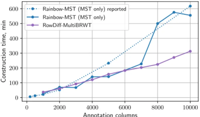
In this section, we compare the construction times for building RowDiff and MST [19] (Figure 3).
The construction time for RowDiff-MultiBRWT includes the RowDiff transform from original columns to the RowDiff format (with the depth pa- rameter set to 100) in addition to the time for con- version of the transformed columns to the Multi- BRWT binary matrix representation. For MST, the time does not include construction of the mapping vector and includes only the time for compression of the unique annotation rows, which is a lower bound on the total construction time for the MST method.
0 2000 4000 6000 8000 10000
Annotation columns 0
100 200 300 400 500 600
Constructiontime,min
Rainbow-MST (MST only) reported Rainbow-MST (MST only) RowDiff-MultiBRWT
Figure 3: Construction time for RowDiff and MST on the RNA-Seq (k=23) data set using 15 cores. The dashed line shows the construction time for MST (with 16 threads) reported in [19].
3.3 Representation size
We now compare the disk footprint for RowDiff and other state-of-the-art graph annotation compression methods.
2000 4000 6000 8000 10000
Number of SRA samples 0
10 20 30 40 50 60
Size,GB
Rainbow-MST
Rainbow-MST (mapping only) MultiBRWT
RowDiff-RowSparse RowDiff-MultiBRWT
(a) RNA-Seq (k=31) data set
2000 4000 6000 8000 10000 12000
Number of taxonomy IDs 0.0
2.5 5.0 7.5 10.0 12.5 15.0
Size,GB
Rainbow-MST
Rainbow-MST (mapping only) MultiBRWT
RowDiff-RowSparse RowDiff-MultiBRWT
(b) RefSeq (Fungi) data set
Figure 4:Annotation size. Rainbow-MST (mapping only) represents the size of the mapping vector compressed as in the Rain- bowfish scheme, and represents a lower bound on the Rainbow-MST representation size. Rainbow-MST computation on the data sets with>4000samples could not be computed because Mantis did not complete within the 10 day limit of our compute cluster.
Figure 4shows the representation size for the RNA-Seq (k=31) and RefSeq (Fungi) data sets. On the RNA-Seq (k=31) data set, RowDiff-MultiBRWT effectively takes advantage of the topology of the graph annotation and the similarity of rows of the annotation matrix and achieves a nearly 4-fold size reduction compared to Multi-BRWT applied on non-sparsified columns. Compared to the Rainbow-MST method, RowDiff-MultiBRWT achieves a 2-fold size reduction. Rainbow-MST computation on the subsets with more that4000samples could not be computed because Mantis did not complete within the 10 day limit of our compute cluster.
On the RefSeq (Fungi) data set, RowDiff takes advantage of the longer stretches of nodes with identical annotations and achieves a 26-fold size reduction relative to Rainbow-MST. Notably, this significant dif- ference comes from the fact that virtually all of the space used by Rainbow-MST is taken by the mapping vector on this data set.
2000 4000 6000 8000 10000
Number of SRA samples 0
20 40 60 80
Size,GB
Rainbow-MST
Rainbow-MST (mapping only) MultiBRWT
RowDiff-RowSparse RowDiff-MultiBRWT
Figure 5:Annotation size for RNA-Seq (k=23).
On the RNA-Seq (k=23) data set, RowDiff- MultiBRWT achieves a 2.5-fold size reduction (Figure 5) relative to Multi-BRWT and a 1.5-fold reduction relative to Rainbow-MST.
The RowSparse format stores the indices of set bits in each row in a compressed integer vector. This type of annotation is faster to construct and to query than the Multi-BRWT representation, but its foot- print is significantly larger on denser datasets, such as RNA-Seq (k=31).
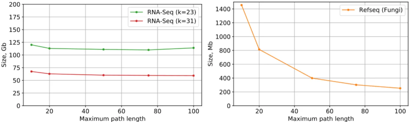
3.4 Effect of the RowDiff depth parameter on size
Section 2.3 introduces the concept of a maximum path lengthM, which ensures that annotation reconstruc- tion time is bounded by a constant. Figure 6 shows the effects of choosing various values for the maximum path length M on the RNA-Seq (k=23), RNA-Seq (k=31), and RefSeq (Fungi) data sets. While setting a shorter maximum path length has negligible effect on the denser RNA-Seq graph, increasing the path length from 10 to 100 reduces the annotation size by a factor of 5.75 on the much sparser RefSeq (Fungi) graph.
20 40 60 80 100
Maximum path length 0
25 50 75 100 125 150 175 200
Size, Gb
RNA-Seq (k=23) RNA-Seq (k=31)
20 40 60 80 100
Maximum path length 0
200 400 600 800 1000 1200 1400
Size, Mb
Refseq (Fungi)
Figure 6:Annotation size vs. max path lengthfor RNA-Seq (k=31) and RefSeq (Fungi).
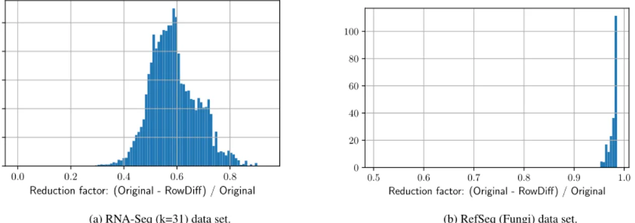
3.5 Compression of single columns
In this experiment, we measure how RowDiff affects the size of the individual columns of the annotation matrix. Figure 7 shows the reduction factor achieved by RowDiff on two datasets representing two different extreme cases of sequence variability.
0.0 0.2 0.4 0.6 0.8
Reduction factor: (Original - RowDiff) / Original 0
1 2 3 4 5
(a) RNA-Seq (k=31) data set.
0.5 0.6 0.7 0.8 0.9 1.0
Reduction factor: (Original - RowDiff) / Original 0
20 40 60 80 100
(b) RefSeq (Fungi) data set.
Figure 7:Column reduction factorweighted with the column size. The columns are stored in SD compressed vectors.
The de Bruijn graph constructed from assembled genomes (RefSeq (Fungi)) contains significantly fewer branches and bubbles than the graph constructed from reads (RNA-Seq (k=31)) and, thus, is significantly better compressed by RowDiff.
3.6 Query performance
In this experiment, we measured the time needed for querying the RNA-Seq (k=23) annotation for human transcripts. The query is performed with the algorithm optimized for long paths (see Section 2.5). First, we construct a list of annotation rows that have to be reconstructed from the RowDiff format and a list of all diff rows for querying in the RowDiff matrix. Then, all these rows are queried and the original annotation rows are reconstructed. Table 1 shows the time taken for reconstruction of the original annotations for 100 and 1000 random human transcripts, which includes the time for querying the diff rows and reconstruction of the original annotations. Since RowDiff requires traversing the de Bruijn graph to get RowDiff paths, the query time for RowDiff depends on the traversal performance of the underlying representation of the de Bruijn graph. In this experiment, we used the succinct de Bruijn graph representation available in MetaGraph [6].
Table 1: Time for querying 100 and 1000 random human transcripts with RowDiff-RowSparse and RowDiff-MultiBRWT. The second column shows the total number of original annotation rows reconstructed for the query. All benchmarks were performed with a single thread on Intel(R) Xeon(R) Gold 6140 CPU @ 2.30GHz.
Query data # rows reconstructed Query time
RowDiff-RowSparse RowDiff-MultiBRWT
100 transcripts 44,995 8.7 sec 38 sec
1000 transcripts 553,280 95 sec 342 sec
4 Conclusions
In this paper, we introduced RowDiff, a new technique for compacting graph labels by leveraging the likely similarities in annotations of nodes adjacent in the graph. We designed a parallel construction algorithm
with linear time complexity in the number of node-label pairs and small memory footprint. In addition, the algorithm can efficiently be distributed and parallelized, making it applicable on arbitrarily large graphs.
RowDiff reduced the size of graph annotations by 2- to 26-fold when used in combination with Multi-BRWT relative to Mantis-MST, the most efficient state-of-the-art representation.
Although the row reconstruction method inevitably leads to an increase inad hocrow query time due to the larger number of required annotation matrix queries, this limitation is alleviated in practice due to the tendency of real-world sequences to featurek-mers which co-occur on matching RowDiff paths.
The optimization of anchor assignment is also a clear direction for future development of these methods.
The anchor assignment method we have presented is designed to reduce the row reconstruction time by setting an upper bound on the traversal length. However, given that there is a trade-off between the size and the query time of the final representation, designing an objective function and a corresponding algorithm to best optimize these measures is a non-trivial task.
Moving beyond the representation of binary relations, a simple extension of the RowDiff method can be used as an efficient way to represent genomic coordinates for indexes of reference genomes. By representing a coordinate at each anchor node, the coordinates of all other nodes in that anchor’s corresponding RowDiff path can be computed via their traversal distance to the anchor.
Each improvement in the compression of sequence graphs and their associated annotations opens up further opportunities for their real-world applicability. When handling large annotations, even a 2-fold difference in the representation size can make a previously unapproachable annotation accessible to the available hardware. With RowDiff, we have demonstrated that there still is great potential for improving the representation of annotations on sequence graphs.
5 Acknowledgements
Mikhail Karasikov and Harun Mustafa are funded by the Swiss National Science Foundation Grant No.
407540 167331 “Scalable Genome Graph Data Structures for Metagenomics and Genome Annotation” as part of Swiss National Research Programme (NRP) 75 “Big Data”.
References
[1] Stephens, Z. D.et al. Big data: astronomical or genomical? PLoS biology13, e1002195 (2015).
[2] Cox, A. J., Bauer, M. J., Jakobi, T. & Rosone, G. Large-scale compression of genomic sequence databases with the burrows–wheeler transform. Bioinformatics28, 1415–1419 (2012).
[3] Ondov, B. D.et al. Mash: fast genome and metagenome distance estimation using minhash. Genome biology17, 132 (2016).
[4] Breitwieser, F., Baker, D. & Salzberg, S. L. Krakenuniq: confident and fast metagenomics classifica- tion using unique k-mer counts. Genome biology19, 198 (2018).
[5] Bradley, P., den Bakker, H. C., Rocha, E. P., McVean, G. & Iqbal, Z. Ultrafast search of all deposited bacterial and viral genomic data. Nature biotechnology37, 152 (2019).
[6] Karasikov, M.et al.Metagraph: Indexing and analysing nucleotide archives at petabase-scale.bioRxiv (2020).
[7] Chikhi, R. & Rizk, G. Space-efficient and exact de bruijn graph representation based on a bloom filter.
Algorithms for Molecular Biology8, 22 (2013).
[8] Benoit, G.et al. Reference-free compression of high throughput sequencing data with a probabilistic de bruijn graph. BMC bioinformatics16, 288 (2015).
[9] Bowe, A., Onodera, T., Sadakane, K. & Shibuya, T. Succinct de Bruijn graphs. InLecture Notes in Computer Science (including subseries Lecture Notes in Artificial Intelligence and Lecture Notes in Bioinformatics)(2012).
[10] Iqbal, Z., Caccamo, M., Turner, I., Flicek, P. & McVean, G. De novo assembly and genotyping of variants using colored de bruijn graphs. Nature genetics44, 226–232 (2012).
[11] Pandey, P.et al. Mantis: A Fast, Small, and Exact Large-Scale Sequence-Search Index. Cell Systems (2018). URLhttp://dx.doi.org/10.1016/j.cels.2018.05.021.
[12] Muggli, M. D.et al.Succinct colored de Bruijn graphs. Bioinformatics(2017).
[13] Raman, R., Raman, V. & Satti, S. R. Succinct indexable dictionaries with applications to encoding k-ary trees, prefix sums and multisets. ACM Transactions on Algorithms (TALG)3, 43–es (2007).
[14] Elias, P. Efficient storage and retrieval by content and address of static files. Journal of the ACM (JACM)21, 246–260 (1974).
[15] Fano, R. M. On the number of bits required to implement an associative memory (Massachusetts Institute of Technology, Project MAC, 1971).
[16] Almodaresi, F., Pandey, P. & Patro, R. Rainbowfish: A Succinct Colored de Bruijn Graph Rep- resentation. In Schwartz, R. & Reinert, K. (eds.) 17th International Workshop on Algorithms in Bioinformatics (WABI 2017), vol. 88 of Leibniz International Proceedings in Informatics (LIPIcs), 18:1–18:15 (Schloss Dagstuhl–Leibniz-Zentrum fuer Informatik, Dagstuhl, Germany, 2017). URL http://drops.dagstuhl.de/opus/volltexte/2017/7657.
[17] Karasikov, M.et al. Sparse binary relation representations for genome graph annotation. Journal of Computational Biology27, 626–639 (2020).
[18] Mustafa, H.et al. Dynamic compression schemes for graph coloring. Bioinformatics35, 407–414 (2019).
[19] Almodaresi, F., Pandey, P., Ferdman, M., Johnson, R. & Patro, R. An efficient, scalable and exact rep- resentation of high-dimensional color information enabled via de bruijn graph search. InInternational Conference on Research in Computational Molecular Biology, 1–18 (Springer, 2019).
[20] Gog, S., Beller, T., Moffat, A. & Petri, M. From theory to practice: Plug and play with succinct data structures. InLecture Notes in Computer Science (including subseries Lecture Notes in Artificial Intelligence and Lecture Notes in Bioinformatics)(2014).
[21] O’Leary, N. A. et al. Reference sequence (RefSeq) database at NCBI: Current status, taxonomic expansion, and functional annotation. Nucleic Acids Research(2016).