Distributed Set Reachability

(1)

Distributed Set Reachability

Sairam Gurajada

Max-Planck-Institute for Informatics Campus E1.4

66123 Saarbrücken, Germany

gurajada@mpi-inf.mpg.de

Martin Theobald

University of Ulm James-Franck-Ring O27

89069 Ulm, Germany

martin.theobald@uni-ulm.de

ABSTRACT

In this paper, we focus on the efficient and scalable processing of set-reachability queries over a distributed, directed data graph. Aset-reachability query is a generalized form of a reachability query, in which we consider two setsSand T of source and target vertices, respectively, to be given as the query. The result of a set-reachability query are all pairs of source and target vertices (s, t), withs ∈ S and t∈ T, wheres is reachable to t(denoted asS ;T). In case the data graph is partitioned into multiple, edge- and vertex- disjoint subgraphs (e.g., when distributed across multiple compute nodes in a cluster), we refer to the resulting set- reachability problem asdistributed set reachability. The key goal in processing a distributed set-reachability query over a partitioned data graph both efficiently and in a scalable manner is (1) to avoid redundant computations within the local compute nodes as much as possible, (2) to partially evaluate the local components of a set-reachability query S ; T among all compute nodes in parallel, and (3) to minimize both the size and number of messages exchanged among the compute nodes.

Distributed set reachability has a plethora of applications in graph analytics and for query processing. The current W3C recommendation for SPARQL 1.1, for example, intro- duces a notion of labeled property paths which resolves to processing a form of generalized graph-pattern queries with set-reachability predicates. Moreover, analyzing dependencies amongsocial-network communities inherently involves reachability checks between large sets of source and target vertices. Our experiments confirm very significant perfor- mance gains of our approach in comparison to state-of-the- art graph engines such as Giraph⁺⁺, and over a variety of graph collections with up to 1.4 billion edges.

1. INTRODUCTION

1.1 Background & Motivation

The reachability problem in directed graphs is one of the most fundamental problems in terms of both graph theory

Permission to make digital or hard copies of all or part of this work for personal or classroom use is granted without fee provided that copies are not made or distributed for profit or commercial advantage and that copies bear this notice and the full cita- tion on the first page. Copyrights for components of this work owned by others than ACM must be honored. Abstracting with credit is permitted. To copy otherwise, or re- publish, to post on servers or to redistribute to lists, requires prior specific permission and/or a fee. Request permissions from permissions@acm.org.

SIGMOD’16, June 26-July 01, 2016, San Francisco, CA, USA c 2016 ACM. ISBN 978-1-4503-3531-7/16/06. . . $15.00

DOI:http://dx.doi.org/10.1145/2882903.2915226

and applications: for a directed graphG= (V, E) with vertices V and edges E, given a source vertexs ∈ V and a target vertex t∈V, determine whether there is a consecutive path of edges fromstotoverE.

To avoid redundant computations, many graph applications in fact require an extension of this basic reachability problem, where entiresetsS,Tof source and target vertices, respectively, need to be processed “at once”. The resulting reachability problem, which we then coin set reachability, aims to retrieve all pairs of source and target vertices (s, t), withs∈S andt∈T, wheresis reachable tot. Moreover, in case the data graph is partitioned into multiple, edge- and vertex-disjoint subgraphs (e.g., when distributed across multiple compute nodes in a cluster), we refer to the resulting set-reachability problem as distributed set reachability (or “DSR” for short). The key goal in processing a DSR query over a partitioned data graph both efficiently and in a scalable manner is (1) to avoid redundant computations within the local compute nodes as much as possible, (2) to partially evaluate the local components of a set-reachability queryS;Tamong all compute nodes in parallel, and (3) to minimize both the size and number of messages exchanged among the compute nodes.

State-of-the-art indexing techniques for reachability queries [12, 16, 18, 25, 28, 32, 33, 34, 36] are largely limited to a centralized setting and thus address only point (1) of the above objectives. As for (2) and (3), we are currently aware of only one approach that specifically tackles the problem of distributed reachability queries for single-source, single- target queries [9]. For multi-source, multi-target (i.e., actual set-) reachability queries, we are aware of just two central- ized approaches [12, 30] that provide suitable indexing and processing strategies. Both are based on a notion ofequiv- alence setsamong graph vertices which effectively resolves to a preprocessing and indexing step of the data graph to predetermine these sets. Efficient centralized approaches, however, are naturally limited to the main memory of a single machine and usually do not consider a parallel—in this case multi-threaded—execution of a reachability query.

Distributed graph engines, such as Google’s Pregel [22], Berkeley’s GraphX [35] (based on Spark [37]), Apache Gi- raph [1] and IBM’s very recent Giraph⁺⁺[31], on the other hand, allow for the scalable processing of graph algorithms over massive, distributed data graphs. All of these provide generic API’s for implementing various kinds of algorithms, including multi-source, multi-target reachability queries. However, a principal assumption we follow in this work is that set-reachability queries are selective. That is,

(2)

for any given setsS, T of source and target vertices, both S and T are usually much smaller than V, while the set of reachable pairs in turn usually is much smaller than the cross-productS×T. Just like in relational approaches, an efficient processing of set-reachability queries thus calls for the aforementioned usage of indexing strategies that take advantage of the salient properties of the data graph. Graph indexing and the processing of selective queries however breaks thenode-centric computingparadigm of Pregel and Giraph, where major amounts of the graph are successively shuffled through the network in each of the underlying MapReduce iterations (the so-called “supersteps”).

Giraph⁺⁺is a very recent approach to overcome this overly myopic form of node-centric computing, which led to a new type of distributed graph processing that is coined graph- centric computingin [31]. By exposing intra-node state information as well as the inter-node partition structure to the local compute nodes, Giraph⁺⁺is a great step towards mak- ing these graph computations more context-aware. How- ever, index structures that specifically tackle the iterative communication rounds required for the supersteps are diffi- cult to accomplish even here, such that a direct implemen- tation of a reachability query may still result in as many iterations (and hence communication rounds) as the diameter of the graph in the worst case.

Finally, the set-reachability problem has a plethora of applications in graph analytics and query-processing tasks.

With its recent update, SPARQL 1.1, for example, under- went a major revision in which the usage of labeled prop- erty paths[2] allows a user to formulate transitive reachability constraints among the query variables. Since both the source and target variables of a property path may become bound to multiple RDF constants at query processing time, the processing of property paths in SPARQL 1.1 resolves to processing set-reachability queries. Another interesting application of set-reachability iscommunity analysis in so- cial networks. That is, given sets of source and target ver- tices, each representing social-net users such as on Twitter or Facebook, we may want to efficiently detect which communities are densely connected. For example, consider two communities—billionaires and non-profit organizations—, it would be interesting to find the list of billionaires who are also involved in philanthropic activities.

1.2 Contributions

We summarize the contributions of our work as follows.

• We formalize the problem of distributed set reachabili- ty (DSR) over a partitioned, and hence distributed, directed data graph. To our knowledge, our approach is the first to specifically tackle this problem.

• We develop a graph-based index structure that allows us to strictly restrict the communication protocol among the compute nodes to asingle round of message exchange in order to resolve the results of any DSR query posed against a given partitioning of the data graph. This guarantee holds regardless of the properties of the data graph (such as its diameter and partition structure) and the properties of the query (such as the distribution of source and target vertices among the graph partitions).

• Our indexing strategy allows forincremental updatesof the underlying data graph, with an efficient support for vertex and edge insertions and a principle support for respective deletions.

• Our approach is alsoextensiblein the sense that any existing, centralized reachability index can be “plugged-in”

at the local compute nodes. We report the results of our distributed approach in combination with a plain DFS search [6], the MS-BFS approach of [30], and FERRARI [28] as local search strategies.

• Moreover, we provide an extensive experimental evalu- ationof our approach over a variety of both small and large graphs and in comparison to different extensions of Giraph⁺⁺. We also investigate two application scenarios of our approach for processing SPARQL 1.1 queries with property paths and for detecting dependencies among social-network communities.

2. PRELIMINARIES

We start by formally defining our data and query model.

This section also serves to establish the notation we will use through the rest of the paper.

Definition 1. Adata graphG(V, E, L, φ)is a directed graph consisting of verticesV and edgesE⊆V×V. Further, we assume a unique label (i.e., an identifier) for each vertex in the graph to be given by a bijective mapping φ:V →L from verticesV to labelsL.

Given two verticess, t∈V, apathPfromstotis denoted by a consecutive set of edges {(s := u0, u1),(u1, u2), . . . , (un−1, un=:t)}such that each (ui, uj)∈E. Two verticess andtare calledreachable, denoted ass;t, iff there exists at least one pathP ⊆E fromstot.

Graph Partitioning. To scale a reachability querys;t to a very large data graph, which may not necessarily fit into the main-memory of a single compute node, we allow the graph to be partitioned intokedge- and vertex-disjoint subgraphs. Formally, asubgraph Gi(Vi, Ei, L, φ) of a data graphG(V, E, L, φ) is a vertex-induced subgraph ofG, such that Vi ⊆V and Ei ={(u, v)|u∈ Vi, v∈ Viand (u, v) ∈ E}. We refer toG={G1, G2, . . . , Gk}as thepartitioningof Gand toC(VC, EC, L, φ) as thecutofG, respectively. Here, k denotes the number of partitions ofGand each partition Gi (includingC) denotes a subgraph of G. Moreover, C is a subgraph of Gsuch that, for a given graph partitioning G,EC ={(u, v)|(u, v)∈E, u∈Vi, v∈Vjandi6=j}with verticesu, v∈VC, iff edge (u, v)∈EC.

Definition 2. Given a partitioningG={G1, G2, . . . , Gk} and the respective cutC(VC, EC, L, φ)of a data graphG, a DSR query, denoted asS;T, returns all pairs of source and target vertices(s, t), withs∈S andt∈T, wheres;t.

Definition 3. For a given graph partitioning G and im- plied cut C of a data graph G, we define the set of in- boundariesIifor partitionGiasIi={v|v∈Vi,∃(u, v)∈ EC, u∈Vj andi6=j}, i.e., as the set of vertices inGi that have an incoming edge from the cutC.

Conversely, we define the set of out-boundaries Oi = {v|v ∈ Vi,∃(v, u) ∈ EC, u ∈ Vjandi 6= j} as the set of vertices inGi that have an outgoing edge into the cutC.

Partitioning Function. We denote byρ : V 7→N⁺0 the partitioning functionthat determines to which of the compute nodes (i.e., “slaves”) in a cluster architecture each graph vertexv∈V is distributed. Without loss of generality, and to simplify notation for the following presentation, we assume a simple partitioning strategy by distributing every

(3)

d e b

f r

a c

g i

l

h k u

n m

p q v

o Slave 1

G1

Slave 2

G2

Slave 3

G3

(a) GraphG

f b e

c g

h i n

m o

G1 G2 G3

(b) CutC Figure 1: (a) GraphGwith partitionsG={G1, G2, G3}and (b) respective cut C

vertexv∈Vi to slavei(i.e.,ρ(v) =ifor eachv∈Vi). We will thus refer to a graph partition and a slave interchange- ably. To increase concurrent executions (e.g., when using multi-threading at the local compute nodes), an “overpar- titioning” strategy may be employed instead, by assigning multiple graph partitions to each of the slaves.

Example 1. Figure 1(a) shows an example graphGwith three partitionsG={G1, G2, G3} which are stored at three slaves. Its corresponding cutCis shown in Figure 1(b). In- and out-boundaries areI1={f}, O1={b, e},I2={c, g, h}, O2={i}, andI3 ={m, n},O3={o}, respectively.

Distributed Reachability. Our approach for processing DSR queries uses a similar setting as described by Fan et al. [9]. In [9], a distributed (single-source, single-target) reachability querys;tover a master-slave architecture is evaluated as follows. The master receivess;tand communicates it to all slaves. At partitionGi, containing the source s, a local evaluation of the reachability ofs to each vertex in the set of out-boundariesOiis computed first. Similarly, at partitionGjcontaining the targett, a local evaluation of the reachability of each vertex in the set of in-boundariesIj

is computed next. Additionally, a local computation of the reachability between all in-boundariesIiand out-boundaries Oi is computed at each partition G1, . . . , Gk and hence at all slavesi= 1..kin the compute clusterin parallel.¹

The resulting local reachability information is encoded into sets of Boolean formulas, where each such set represents the local connectivities between the in-boundaries Ii

(including the sources, if present) with the out-boundaries Oi (including the target t, if present) at partition Gi. All of these formulas are communicated back to a single master node for the final evaluation. A query-specificglobal depen- dency graph is constructed at this master node for s ; t using the Boolean formulas and the static cutC. A reachability algorithm is then run over the dependency graph to answers ;tvia substitution of the variables that are re- versely connected to the target vertex t. The overall algorithm provided in [9] can be implemented with a simple communication protocol and, for example, be executed in a single MapReduce iteration among all compute nodes.

Example 2. Consider the distributed reachability query d;q over the graph partitioning shown in Figure 1. The local evaluation at each partition results in the following Boolean representation of partial reachability information:

{d = b∨e, f = b∨e}@G1, {c = i, g = i, h = i}@G2, {m=q∨o, n=q∨o}@G3. By including the edges in the cut C (Figure 1(b)), the global dependency graph (Figure 2(a)) is constructed at the master node to finally resolved;q.

By running a reachability algorithm (such as backward DFS)

1Note that we follow a slightly different definition of in- and out-boundaries than in [9]. However, the algorithm in [9]

directly translates to the one outlined above.

f d

b e

g c

h

i n

m

o q

(a) Single Reachability

Master

f d

a b e

g c

h ii l

n m

o p

(b) Set Reachability

Master

Figure 2: Dependency graph as constructed in [9]

for a single reachability query (a) and an extension to set reachability (b)

over the dependency graph, one can find thatd;qis indeed true(the red path in Figure 2(a)).

3. DISTRIBUTED SET REACHABILITY 3.1 Naïve Approach

A naïve approach to extend the distributed reachability problem to sets of verticesS,T would be to simply invoke a separate reachability querys;tfor every pair (s, t), with s∈Sandt∈T. However, an obvious reason for the limited efficiency of this approach, even for reasonably-sized setsS andT, is that this approach does not exploit the assumption we made earlier, namely that queries areselective, i.e., that by far not all pairs inS×Tare reachable. Consequently, this approach can also not reuse any intermediate computations and thus likely performs many redundant computations.

3.2 DSR with a Dynamic Dependency Graph

Animproved approachto extend the distributed reachability algorithm provided in [9] to sets is as follows. LetS;T be the query received at the master. First, we partition S ;T into subqueries S1 ;T1, S2 ;T2,. . .,Sk ;Tk, where k is the number of graph partitions, such that each Si⊆Vi andTi⊆Vi contains only vertices that are local to partitionGi. Next, a local evaluation at each slaveiinvolves finding the reachability among all pairs of vertices from the sets Si∪Ii andOi∪Ti, respectively. These can again be runin parallel across all slaves. The resulting reachability information, again represented as sets of Boolean formulas, is then communicated from all slaves to the master node for the final evaluation. At the master node, the query-specific dependency graph for the sets S, T is constructed as described in Section 2, and a local reachability algorithm is then used at the master node to emit all reachable pairs (s, t), withs∈S andt∈T.

Example 3. Consider the DSR queryS ;T with S = {a, d, g}andT ={l, p}over the cutCshown in Figure 1(b).

The sets of Boolean formulas obtained after the local evalu- ation at each slave are as follows: {a=b∨e, d=b∨e, f= b∨e}@G1, {c=i, g =i∨l, h=i}@G2, {m=p∨o, n= p∨o}@G3. At the master node, after evaluating S ; T over the global dependency graph shown in Figure 2(b), we obtain the following reachable pairs of source and target ver- tices: {(a, l),(a, p),(d, l),(d, p),(g, l),(g, p)}.

(4)

3.2.1 Discussion

Although the second algorithm provides a more viable so- lution of the DSR problem than the naïve approach, it still leaves a number of disadvantages that limit both its efficiency and scalability.

• First, the query-dependent, global dependency graph is generated “from scratch” for each query S ; T, although both the cut Cand the local reachability information Ii ; Oi among the in- and out-boundaries at each graph partitionGi are in fact static.

• Second, the approach does not leverage any distributed computation in its second step, as the final reachability computation S ;T over the global dependency graph is performed only by a single master node.

• Third, since the global dependency graph is generated dynamically for each queryS ;T, a reachability index for the static cut C and the local Ii;Oi components cannot be constructed, which restricts the final reachability computation to either a simple BFS or DFS strategy over the dependency graph.

3.3 DSR with a Static Reachability Index

Inour approach, instead of computing the global dependency graph for each incoming query from scratch at the master node, we precompute a partition-specific variant there- of, called the “boundary graph”, only once and store this in the form of a static reachability index at each slave. This strategy provides multiple benefits. First, it avoids repeated computations of the boundary graph for each query. Second, since each slave has the complete reachability information among the boundary vertices of all other slaves available, finding the reachability of any two vertices (s, t) in the en- tire data graphGresolves to a local reachability computation at at most two slaves, which is irrespective of the diameter of the graph and the distribution of the source and target vertices of a set-reachability query (see Theorems 1 and 2). Additionally, an index can be built over the static boundary graph to accelerate this processing. Third, storing a (compacted version of the) boundary graph at each slave allows for a fully distributed processing of a set-reachability query and thus avoids the single-node bottleneck of previous approaches. We next formally define how we generate the boundary graph and its derived index structures.

3.3.1 Precomputed Index Structures

Boundary Graph. Aboundary graphis a directed graph that represents the reachability information among the in- and out-boundaries of all graph partitionsG={G1, . . . , Gk} with respect to a given cutC.

Definition 4. Let G^B_i (V_i^B, E_i^B,L, φ) denote the boun- dary graphwe compute for partitionGi, such that the fol- lowing holds:

• The verticesV_i^B=S

i=1..kIi∪Oiconsist of the union of all in- and out-boundaries of all partitionsG1, . . . , Gk.

• There exists an edge(u, v)∈E^B_i , iff - (u, v)∈EC, or

- u∈Ij andv∈Oj, forj6=i, andu;v(i.e.,uand v are both located at another partitionGj and there exists a path fromutovinGj).

That is, the boundary graph for partitionGi merges the static cutCwith the static reachability informationIj;Oj

f b

e g c

h

i n

m

o

(a) Non-optimized

Slave 1

G^B1

f b

e υ3 ν2

υ2 ν3 υ4

ν4

−

→c

−

→h −→m

−

→n

(b) Optimized

Slave 1

G^B1

Figure 3: Boundary graphG^B1 for partitionG1

among all the remaining graph partitionsGj(fori6=j) into a new, precomputed graph G^B_i. The resulting boundary graphs are thus partition-specific.

Example 4. For our graphGwith partitionsG1,G2,G3

and respective cut C as shown in Figure 1, the boundary graph G^B₁ for partitionG1 is shown in Figure 3(a). Here, the dashed edges refer to edges in the cutC, while the solid edges denote the transitive reachabilityIj;Oj (forj6= 1).

Complexity. The construction of the boundary graph requires us to materialize the pairwise reachability Ii ; Oi

among the in- and out-boundaries for each partitionGi. Us- ing a simple BFS/DFS-based approach, the time complexity of this computation isO((|Vi|+|Ei|)·|Ii|·|Oi|) per partition.

This can be further improved toO(1· |Ii| · |Oi|) when using a sophisticated, local reachability index for this operation.

On the other hand, the (worst-case) space complexity for storing the boundary graph at partition iis O(Pk

j=1|Ij| ·

|Oj|+|EC|), for j 6= i. From this, one can deduce that both the time and space complexity of the boundary graph computation strongly depend on the amounts of in- and out- boundaries we obtain from the cutC.

Min-k-Cut Partitioning. A standard approach to reduce this number of boundary vertices is to reduce the number of edges in the cutC, while trying to keep the sizes of the partitions G1, . . . , Gk balanced. Although finding an optimal such min-k-cut partitioning is a well-known NP-complete problem [6], current graph libraries such as METIS [17]

are capable of achieving very good approximations even for graphs with hundreds of millions of edges.

Equivalence Sets. Even for a given cutC, we can further reduce the size of the boundary graph by grouping the in- and out-boundary vertices intoequivalence setsof vertices, thus continuing the idea presented in [12] to a distributed setting. Specifically, we achieve this by grouping the boundary vertices into forward- andbackward-equivalent sets according to the following definition.

Definition 5. Two in-boundaries b1, b2 are called for- ward-equivalentwith respect to subgraphGi, i.e.,b1≡^f b2, iff for any vertexv∈Vi−Iiandb1;v, it holds thatb2;v.

Conversely, two out-boundariesb1, b2are calledbackward- equivalentwith respect to subgraphGi, i.e.,b1≡^bb2, iff for any vertexv∈Vi−Oiandv;b1, it holds thatv;b2.

That is, once the forward- and backward-equivalent sets of vertices are identified for each subgraph Gi, each such set is replaced by a newin-virtual vertex υ (for a forward- equivalent set) and a newout-virtual vertexν(for a backward- equivalent set), respectively.

Example 5. Following the above definition of equivalence for the partitioning G = {G1, . . . , G3}of G shown in Fig- ure 1(a), we can obtain the following, partition-specific equiv- alence sets: {υ1 = {f}}@G1, {ν1 = {b, e}}@G1; {υ2 =

(5)

d e b

r f a

υ3

υ2

ν2

ν3

υ4

ν4

−

→c

−

→h

−

→n

−

→m Slave 1

G^C1

c

g i

l

h k u ν1

υ1

υ4

ν4

←− b

←−e

−

→n

−

→m Slave 2

G^C2

n m

p q v

o ν3

υ3

υ1

ν1 υ2 ν2

−→c, h

←−b, e

Slave 3

G^C3

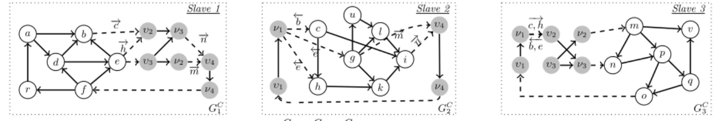
Figure 4: Final compound graphsG^C₁, G^C₂, G^C₃ constructed for graph Gwith cutC of Figure 1 {c, h}, υ3 = {g}}@G2, {ν2 = {g}, ν3 = {i}}@G2; {υ4 =

{m, n}}@G3,{ν4={o}}@G3.

Next, the in- and out-boundaries are redefined with respect to the new virtual vertices. That is, Ii comprises of all in-virtual vertices andOicomprises of all out-virtual vertices. The optimized boundary graph for partition G1 is shown in Figure 3(b). Note that we attach additional labels to the cross-edges in the boundary graph to obtain a loss- less representation of the boundary graph with respect to the partitionsG1, . . . , Gk. For example, the cross-edge (b, c) is represented by connecting the vertexband the in-virtual vertexυ2 with the label−→c to denote thatbis connected to onlycinυ2. The forward arrow denotes that this connec- tion is valid only for a forward exploration. This is required, since verticesc,hare forward-equivalent, i.e.,c≡^f h, with respect to partitionG2 only.

Computing Equivalence Sets. According to Definition 5, two in-boundariesb1∈Iiandb2 ∈Iiare forward-equivalent if they are reachable to exactly the same set of vertices in Vi−Ii. To determine the sets of forward-equivalent boundaries, we need to (1) compute all reachable pairs from Ii

to Vi−Ii and then (2) group the vertices in Ii into these equivalence sets. For large setsIiand Vi−Ii, this computation may be prohibitively expensive. To address (1) and thus reduce the input that needs to be considered for (2), we apply the following optimizations.

• b1,b2can only be forward-equivalent with respect to partition Gi if both belong to the samestrongly connected component (SCC) in Gi. We thus condense Gi into a more compact DAG by computing the SCCs overGi.

• Instead of considering all target verticesVi−Ii, we consider only the direct successors S(Ii) of Ii, and hence S(Ii)−Ii, to check for forward-equivalence. The intu- ition for considering only successors is that if two boundaries b1,b2 are reachable to the same set of vertices in S(Ii)−Ii, thenb1,b2 also are reachable to the same set of vertices inVi−Ii.

A similar construction then holds also for backward-equivalence, except thatpredecessorsP(Oi) are considered instead.

Example 6. Consider partitionG3 with in-boundary set I3 ={m, n} to compute the sets of forward-equivalent ver- tices in I3. In this case, this requires us to only verify whether m≡^f n, sincem, nare the only in-boundaries in I3. First, we run the SCC algorithm to condense G3 into the DAG G⁰3. In this example, G⁰3 = G3, and we see that m, n do not belong to the same SCC. We then check their forward-equivalence based on the sets of vertices inV3−I3

that are reachable from both m and n. To compute these reachable sets of vertices, we consider only the direct suc- cessors S(I3)−I3 = {p, v} instead of considering all of V3−I3 = {p, o, q, v}. Thus, the reachable set of vertices of bothmandnis{p, v}, and hence we have m≡^f n.

A compact algorithm for computing these equivalence sets is depicted in Appendix 8.1.

Compound Graph. After compacting the partition-specific boundary graphs G^B_i by replacing both the forward- and backward-equivalent sets of vertices with their in- and out- virtual counterparts, we perform one more step to obtain our final graph index for evaluating DSR queries. To do so, we merge the partition-specific boundary graphs with the local partitions into acompound graphG^C_i for each partitionGi. These compound graphs will facilitate the processing of DSR queries via a combination of local reachability computations and a single filtering step among these local results.

Definition 6. Let G^Ci(Vi^C, Ei^C,L, φ) denote the com- pound graph we compute for partition Gi, such that the following holds:

• The vertices V_i^C =Vi∪V_i^B consist of the union of ver- tices in the local subgraphGi and boundary graphG^B_i .

• The edges E_i^B =Ei∪E_i^B consist of the union of edges in the local subgraph Gi and boundary graphG^B_i. Figure 4 shows the compound graphs for the initial data graphGfrom Figure 1(a).

Forward- and Backward-Lists. Our last precomputa- tion step consists of storing the forward- and backward-lists, Fi and Bi, of boundaries which are non-local to each partition Gi. These will serve for routing messages to only those partitionsGjwhich are connected toGi. Specifically, the forward-list Fi =S

j6=i{υ|υ is in-virtual vertex ofGj} is the set of all vertices that are non-local to Gi and are in-virtual vertices of another partition Gj. Similarly, the backward-listBi=S

j6=i{ν|ν is out-virtual vertex ofGj} consists of all out-virtual vertices that are non-local toGi. For instance, for partition G1 shown in Figure 4, we have F1={υ2, υ3, υ4}andB1={ν2, ν3, ν4}.

3.3.2 Evaluating DSR Queries

Given these precomputed index structures, i.e., the compound graphs G^C_i and respective forward- and backward- lists,FiandBi, evaluating a DSR query now becomes straight- forward. We again begin with a discussion of the single- source, single-target case and then explain how it generalizes to the multi-source, multi-target case.

A. Single Reachability. Consider the reachability query s;t. The algorithm for processing the query is shown in Algorithm 1. Given a data graph G with partitioning G, we evaluate the query as follows. If bothsandtbelong to same partitionGi, then the reachability s; tis confined to only slaveiwhich stores the compound graphG^Ci. Since the compound graphG^C_i augments eachGi with the global reachability information among all boundary vertices, we can safely evaluate the reachability ofs;tonG^C_i by calling any centralized reachability algorithm via the function localSetReachability(.) (Lines 11-13). A formal justification for this is provided by the following theorem.

Theorem 1. Let s, t both be local vertices of partition i, i.e., s, t ∈ Vi. Then the evaluation of the reachability

(6)

Algorithm 1:Distributed Reachability Processing Input:Compound graphs: {G^C₁, G^C₂, ..., G^C_k}, Query: s;t Output: true/false

1 Master:

2 ranks:=ρ(s) .i.e.,s∈ViandGiis at Slaveρ(i)

3 rankt:=ρ(t) .i.e.,t∈VjandGjis at Slaveρ(j)

4 result:=false

5 foreachrank do

6 result:=result∨compute(s, ranks, t, rankt) .invokes parallel computations at all ranks

7 returnresult

8 Slavei:

9 methodcompute(s,ranks,t,rankt):

10 rset:=∅

11 ifranks=iandrankt=ithen .invoke local reachability evaluation

12 if localSetReachability({s},{t})6=∅then

13 returntrue

14 else if i=ranksthen

15 j:=rankt

16 Υ^js:=localSetReachability({s},F_i^j);

. F_i^j⊆Fiis the set of in-virtual vertices local toj

17 rset[s] := Υ^js 18 sendMessage(j,rset)

19 returnfalse

20 else if i=ranktthen

21 receiveMessage(i,rset)

22 Υⁱ_s:=rset[s]

23 forυinΥⁱ_sdo

24 b:=υ.rep . bis a member vertex in eqsetυ

25 iflocalSetReachability({b},{t})6=∅then

26 returntrue

27 returnfalse

s;tover graphGcan be answered entirely locally over the compound graphG^C_i without requiring any message exchange among the compute nodes.

Proof. See Appendix 8.2.1.

Example 7. Consider the queryb;f. Both verticesb, fare local to partitionG1. By considering only the subgraph G1, one cannot find thatf is reachable fromb. But by con- sidering the whole graphG, we see thatb;f istruevia the pathb→c→i→n→p→o→f. However, using the local compound graphG^C₁ (see Figure 4), we can indeed find that b;f istruevia the pathb→υ2→ν3→υ4→ν4→f.

If, on the other hand, s and t are located at two different partitions Gi, Gj, with i 6= j, the evaluation of a reachability query works as follows (Lines 14-25). Starting at partition Gi, we find the reachability from s to all the forward-boundaries υ ∈ F_i^j ⊆ Fi (Line 15) which are located at another partitionGj. Let Υ^js ⊆ Fi be the set of in-virtual vertices located at partitionGj(and hence stored by slavejas per our assumption) which are reachable from s. The message rset[s]:=hs,Υ^jsi is then communicated to slavej. At slave j, we consider each υ ∈ Υ^j_s and replace it with any one of its membersb, after which we evaluate the reachability frombto the local target vertext. If there exists one suchb∈υ∈Υ^jswithb;t, we report thats;t istrue(Lines 22-25).

Theorem 2. Lets ∈ Vi and t∈ Vj, with i6=j. Then, the evaluation of the reachabilitys;tcan be answered over the two compound graphsG^Ci andG^Cj by using a single step of message exchange from slaveito slavej.

Proof. See Appendix 8.2.2

Example 8. Consider the querya;q, whereais located at partitionG1 andqis located at partitionG3. At partition G1, we compute the reachability fromato the single forward- boundary{υ4}which is located at G3. From the compound graph G^C1 (shown in Figure 4), we have Υ³a = {υ4} since a;υ4. Υ³ais then communicated to slave3. At slave3, we expand the actual vertices represented by the virtual vertex υ4 (say m, since m∈υ4) and find the reachability from m toq. Since m;q, we thus find thata;q istrue.

B. Set Reachability. An actual DSR queryS;T, which is received by the master node, is processed in our approach as shown in Algorithm 2. First, S ;T is partitioned into subqueries S1 ; T1, S2 ; T2,. . ., Sk ; Tk, where k is again the number of graph partitions. The partitioning of the query into these subqueries is determined such that each source vertexsi∈Siand target vertexti∈Tiresides locally at partitionGi(Line 2).

Step 1. (Lines 13-19) A local evaluation at partitionGi

involves processing the pairwise reachability among the vertices fromSi toTi and from Si toFi atall slaves i= 1..k in parallel. This operation generates two types of reachable pairs: (si, ti) and (si, υj). The first type denotes the reachability between both a local sourcesi∈Siand a local target ti∈Ti. The second type denotes the reachability between a local sourcesi∈Si and a forward-boundaryυj∈Fi, which is represented by an in-virtual vertex located at slavej.

Step 2. (Lines 21-32) The communication of the remotely reachable pairs, each of the form (si, υj), is performed from slave i to slave j among all pairs of slaves i, j = 1..k in parallel. In order to reduce the overhead of communicating individual pairs, each slave buffers its partial reachability information and communicates this buffer at once. Each buffer sent from slaveito slavejis of the form{hsi,Υ^j_s_ii}

for allsi∈Si. For easier processing, the messages received at slave i from all other slaves are stored in an inverted indexIi(Υⁱ∗, Li), where Υⁱ∗is the aggregated set of in-virtual vertices (local to slavei). For each in-virtual vertexυ∈Υⁱ∗, its aggregated non-local source setSυ ⊆S is stored in Li. That is, fors∈Sυandυ∈Υⁱ∗, we already know thats;υ.

Step 3. (Lines 34-39) A final local evaluation involves processing the set reachability Υⁱ∗;Tifrom the in-virtual vertices Υⁱ∗ to the target sets Ti at all slaves i = 1..k in parallel. For each in-virtual vertex υ ∈ Υⁱ∗ and original vertexbrepresented byυ, we evaluate the reachability from bto all targetst∈Ti. Ifb;tistrue, then for eachs∈Sυ, we report thats;tistrue.

Example 9. Consider again the graphGwith partitions G1,G2,G3 in Figure 1(a). The respective compound graphs G^C1,G^C2,G^C3 are shown in Figure 4. LetS={d, l, p};T = {a, k, q}be the DSR query received at the master node. The query is partitioned into{d};{a},{l};{k},{p};{q}.

At partition G1, we find the set-reachability (Step 1) be- tween{d},{υ2, υ3, υ4, a}, thus returning the reachable pairs {(d, υ2), (d, υ3), (d, υ4), (d, a)}. We perform the same op- eration in parallel at slaves 2 and 3 and communicate the results to all other slaves (Step 2). At slave 1, we receive

(7)

Algorithm 2:Distributed Set-Reachability Processing

Input:Compound graphs{G^C₁, G^C₂, ..., G^C_k}, Query:S;T Output:R {(s, t)|s∈S, t∈Tands;t}

1 Master:

2 partitionS, Tinto{(S1, T₂),(S₂, T₂), . . . ,(S_k, T_k)}

.whereS_i⊆V_iandT_i⊆V_i

3 result:=∅

4 fori= 1. . . kdo

5 result:=result∪compute(S_i,T_i)

7 Slavei:

8 methodcompute(Si, Ti):

9 local_rset:=∅

10 remote_rset:=∅

11 result:=∅

12 // Step 1:

13 local_rset:=localSetReachability(S_i,T_i)

14 remote_rset:=localSetReachability(S_i,F_i)

15 fors in S_ido

16 fort in local_rset[s]do

17 result:=result ∪ {(s, t)}

18 forυ in remote_rset[s]do

19 Υ^j_s:= Υ^j_s ∪υ

. υis an in-virtual vertex of partitionj

20 // Step 2:

21 forj= 1tokdo

22 ifj6=ithen

23 msg:=∅

24 fors in Sido

25 msg:=msg ∪ {hs,Υ^j_si}

26 sendMessage(j, msg)

27 Ii(Υⁱ_∗, Li) =∅

28 forj= 1tokdo

29 receiveMessage(j,msg)

30 forhs,Υⁱ_siin msgdo

31 forυ inΥⁱ_sdo

32 I_i[υ] :=I_i[υ] ∪ {s}

33 // Step 3:

34 forυ inΥⁱ_∗do

35 b:=υ.rep

36 local_rset:=localSetReachability({b},T_i)

37 fors inIi[υ]do

38 fort ∈ local_rset[b]do

39 result:=result ∪ {(s, t)}

the following reachability information: {(υ1,[l, p])}. Simi- larly, at slave2, we receive {(υ2,[d, p]),(υ3, [d, p])}; and at slave3, we receive{(υ4,[d, l])}. At the end of the local evalu- ation from boundaries to the final targets (Step 3), by replac- ing virtual vertices with each of their represented vertices (at slave1,υ1 is replaced withf), the sets{(d, a),(l, a),(p, a)}@

G1,{(d, k),(l, k),(p, k)}@G2 and{(d, q),(l, q),(p, q)}@G3of reachable pairs are generated at the partitions.

Local Reachability Evaluation. Algorithms 1 and 2 both require partial reachability processing at each slave via the functionlocalSetReachability(.). For this, any centralized reachability index (see, e.g., [6, 28, 12, 36]) can be plugged into our framework. We abstract this by calling localSetReachability(.) in our algorithms whenever a local (set-)reachability operation is invoked.

Forward vs. Backward Processing. Our above discussion focused on starting from the source vertices and ending at the target vertices. If there are less targets than sources, one may also start from the target vertices and search back-

wards to the source vertices to arrive at the same results.

We therefore maintain both forward- and backward-lists,Fi

andBi, to facilitate these two directions of searching.

3.3.3 Incremental Updates

Insertions. Insertions over the SCC-condensed compound graphsG^C_i can be implementedwithoutstoring the original (i.e., uncondensed) compound graphs.

Let (u, v) denote a new edge that is to be inserted into the graph G. First, assume both u and v belong to the same graph partitioni. Further, ifu,vbelong to the same SCC, then adding (u, v) toGi would not change the local compound graphG^C_i (nor any other) at all and thus can be safely ignored. If, on the other hand, u, v belong to two different SCCs, then a series of update actions are required.

First, we add the new edge to the local compound graphG^C_i and locally recompute the SCCs and equivalence sets. Next, new connections among the local in- and out-boundaries,Ii

andOi, are communicated to all other partitionsj(forj6=i) as additional edges. These can be incrementally merged into all the compound graphs G^Cj by updating their SCCs as well. Second, ifu and vbelong to two different partitions i and j, then this means we have a new edge in the cut C, which however does not affect the reachability within partitionsiandj. Thus, (u, v) can directly be merged into the distributed compound graphs as described above.

Letn,mdenote the number of vertices and edges in the condensed compound graph G^Ci , and let |Ii|, |Oi| be the number of in- and out-boundaries for partition i, respec- tively. By adding a local edge to partitioni, a partial or full recomputation of the connections among vertices fromIito Oiis required. Thus the worst-case time complexity of this step isO((n+m)· |Ii| · |Oi|), which is asymptotically optimal [7]. The SCC recomputation at each compound graph has a time complexity ofO(n⁰+m⁰), wheren⁰ andm⁰ are the numbers of vertices and edges in the newG^C_i’s.

Deletions. Deletions over the SCC-condensed compound graphsG^C_i, on the other hand, result in a decremental main- tenance of the SCCs, which requires either storing the original (i.e., uncondensed) compound graphs or organizing the SCCs in a hierarchical manner [19]. In our implementa- tion, we resort to storing the uncondensed compound graphs along with the condensed compound graphsG^C_i, albeit approaches like [19] may be employed for further optimizations.

A deletion of a local edge (u, v) in partitioniis processed over the condensed compound graphG^Ci as follows. If the verticesu,vbelong to the same SCC, then we expand this SCC into its original edges and reconnect these edges to the remaining SCCs inG^Ci. Moreover, in case of deletions, some of the existing boundaries may not be connected any- more. We identify such pairs of boundaries and communicate these to the other compute nodes. After receiving this list of deleted boundary edges, we reconstruct the local compound graphs G^C_j (forj 6= i) analogously to the insertion case. If, on the other hand, the verticesu,vbelong to two different SCCs, then we expand both of them.

Here, the worst-case time complexity to maintain the local boundary edges is O((|Vi|+|Ei|)· |Ii| · |Oi|), which is the same as for rebuilding the local boundary graphs (see Section 3.3.1). The new compound graphs are condensed via SCC computation, whose worst-case time complexity is O(n⁰+m⁰), wheren⁰ andm⁰ again are the numbers of vertices and edges in the newG^C_i’s.