1
Assessments of 48 simulated and 159 real stocks with a Monte Carlo and Bayesian Implementation of a Surplus Production Model
Rainer Froese, Nazli Demirel, Gianpaolo Coro, Kristin M. Kleisner and Henning Winker Corresponding Author: Rainer Froese, GEOMAR, Kiel, Germany, rfroese@geomar.de
Version of June 23, 2016
Supplement for Froese, R., Demirel, N., Coro, G. Kleisner, K.M., Winker, H., Estimating fisheries reference points from catch and resilience, accepted by Fish and Fisheries in July 2016.
Available from http://oceanrep.geomar.de/33076/
Table of contents
Introduction………3
Material and Methods………3
Selection of real stocks ……….4
Generation of simulated stocks………..………....4
Default rules for biomass priors………6
General settings……….6
Rules for the initial prior biomass range………..………6
Rules for the intermediate prior biomass range…….….………..6
Rules for the final prior biomass range……….….………7
CMSY analysis……….7
BSM analysis ………..8
Explanation of graphical CMSY and BSM output………8
Results………..13
CMSY and BSM results compared with “true” values from simulated data……….13
Comparison of CMSY and BSM parameter estimates for 128 fully assessed stocks…………16
2
CMSY and BSM results compared with “true” values from simulated CPUE data…………..28
Comparison of CMSY and BSM parameter estimates for 31 data-limited stocks…….………30
References……….32
Appendix I: Simulated stocks with catch and biomass ..………33
Appendix II: Fully assessed stocks……….57
Region: Alaska……….……….57
Region: Pacific………..77
Region: Northwest Atlantic……….92
Region: Caribbean / Gulf of Mexico……….105
Region: Northeast Atlantic, ICES Area………108
Region: Mediterranean………170
Region: Black Sea……….173
Region: South Africa………..176
Appendix III. Simulated CPUE stocks……….185
Appendix IV. Data-limited stocks with catch or landings and CPUE………209
Appendix V: Landings vs catches………..271
3
Introduction
This Supplement details the results of applying a Monte Carlo algorithm (CMSY) and a Bayesian state-space implementation of the Schaefer surplus production model (BSM) to 48 simulated and 159 real stocks. The respective R-code and the data files are available as online material. The selection of the real stocks, the generation of the simulated stocks, and the settings used in the CMSY analysis are detailed below. The graphical output of the CMSY and BSM analyses is explained in general before the results are presented in summary tables and in detail in Appendices I to IV.
Material and Methods
Table S1 contains the names and a short description of the content of the files that were used in the context of this study. All files are available for download at http://oceanrep.geomar.de/33076/.
Table S1. List of files that were used in the context of this study, with indication of file name and description of content.
File name Content
AllStocks_ID20.csv Stock descriptions, priors, official reference points AllStocks_Catch16.csv Time series of catch and biomass or CPUE
AllStocksResults_6.xlsx Spreadsheet behind the results in Table S5 and S6
CMSY_45y.R R-code implementing CMSY and BSM for simulated stocks CMSY_46e.R R-code implementing CMSY and BSM for real stocks CMSY_46eFig1.R R-code used to create Figure 1 in the main text CMSY_46eFig2.R R-code used to create Figure 2 in the main text CMSY_46eFig3.R R-code used to create Figure 3 in the main text CMSY_46eFig4.R R-code used to create Figure 4 in the main text CMSY_46eFig5-6.R R-code used to create Figures 5 and 6 in the main text CPUEStocks_Results_6.xlsx Spreadsheet behind the results in Table S9 and S10 SimCatch_6.csv Time series of simulated catch and biomass
SimCatchResults_6.xlsx Spreadsheet behind the results in Table S3 and S4 SimCatchCPUE_6.csv Time series of simulated catch and CPUE
SimCatchCPUE_Results_6.xlsx Spreadsheet behind the results in Table S7 and S8
SimSpec_6.csv Priors and “true” parameters for simulated stocks with biomass SimSpecCPUE_6.csv Priors, “true” parameters for simulated stocks with biomass and CPUE SimCatchGenerator_6.xlsx Spreadsheet with algorithm to create simulated stocks with biomass SimCatchCPUEGenerator_6.xlsx Spreadsheet with algorithm to create simulated stocks with CPUE
4
Selection of real stocks
Altogether 128 fully assessed stocks with biomass estimates, 29 data-limited stocks with CPUE data, and two stocks without abundance data were used for the evaluation of the CMSY method. Catch and biomass data were extracted from stock assessment documents that are available online or were provided by the respective assessment bodies. Sixty-two fully assessed stocks from the Northeast Atlantic were obtained from the ICES Stock Summary database and from ICES Advice reports published in 2015 at http://ices.dk. U.S.-managed stocks from the East Pacific and West Atlantic had assessment reports with catch and total biomass estimates available online and were included in the analysis (AFSC 2011; 2012; www.st.nmfs.noaa.gov/sisPortal/sisPortalMain.jsp). Data for six stocks were obtained from working group reports for the Mediterranean and Black Sea (FAO- GFCM, ICES 2014c; JRC 2012). Data for fifteen stocks from the Pacific Ocean were found (BillfishWG–
ISC, ISC 2015; www.st.nmfs.noaa.gov/sisPortal/sisPortalMain.jsp) and nine stocks from South Africa (Winker et al., 2012; ICCAT 2015) were made available and included in the analysis. Catch and CPUE for data-limited stocks from the Northeast Atlantic were obtained from ICES advice reports and from the WKLIFE IV workshop held on 27-31 October 2014 in Lisbon, Portugal (ICES 2014a). Files
containing the time series data for these stocks and the respective meta-data and priors are available as part of the online material (see Table S1).
Generation of simulated stocks
In order to compare parameter estimates of CMSY and BSM with “true” values, stocks with catch and biomass or catch and CPUE were simulated with a time range of 50 years and a fixed k value of 1000. The values for r were drawn randomly from a normal distribution with mean and standard deviation as shown in Table S2. A parameter estimate was considered as “good” if it contained the respective “true” value within its confidence limits (Hedderich and Sachs 2015).
Table S2. Means and standard deviations used for generating normal distributions from which r values were selected randomly for use in simulations.
Resilience r range mean sd High 0.6 – 1.5 1.05 0.15 Medium 0.2 – 0.8 0.5 0.1 Low 0.05 – 0.5 0.275 0.075 Very Low 0.015 – 0.1 0.0575 0.0142
The goal was to create a range of biomass scenarios, including strongly as well as lightly depleted stocks, with monotone stable or monotone changing (i.e., steadily decreasing or increasing) or with alternating biomass trajectories: patterns of high-high (HH), high-low (HL), high-low-high (HLH), low- low (LL), low-high (LH), and low-high-low (LHL) biomass trends. Simulated stocks have names that indicate the combination of biomass trajectory and intrinsic growth rate, e.g., HH_L signifies a stock
5
with monotone high biomass and low resilience. Resilience categories were translated into r ranges as shown in Table S2. The biomass trajectories were created by using the fixed k value, a randomly selected r value (see Table S2), and an initial biomass. The biomass in subsequent years was then generated from a Schaefer model according to Equation S1.
𝐵𝐵𝑡𝑡+1 =𝐵𝐵𝑡𝑡+𝑟𝑟 �1−𝐵𝐵𝑘𝑘𝑡𝑡� 𝐵𝐵𝑡𝑡 𝑒𝑒𝑠𝑠1− 𝐶𝐶𝑡𝑡 𝑒𝑒𝑠𝑠2 (S1)
where Bt+1 is the exploited biomass in the year t+1, Bt is the biomass in the current year t, Ct is the catch in year t, and es1 and es2 are bias-corrected lognormal errors. Note that the error term s1 was assigned to the estimation of the surplus production, i.e., to the interaction process of Bt, r and k, and the second error term s2 was assigned to the catch, representing observation error for the purpose of creating simulated data and for the purpose of CMSY analysis, where abundance is not observed.
If biomass falls below 0.25 k, a linear decline in recruitment towards zero at zero k is assumed and a respective multiplier 4 Bt/k resulting in 1 at 0.25 k to zero at zero k is applied to the surplus
production term as shown in Equation S2.
𝐵𝐵𝑡𝑡+1 =𝐵𝐵𝑡𝑡+ 4𝐵𝐵𝑘𝑘𝑡𝑡 𝑟𝑟 �1−𝐵𝐵𝑘𝑘𝑡𝑡� 𝐵𝐵𝑡𝑡 𝑒𝑒𝑠𝑠1− 𝐶𝐶𝑡𝑡 𝑒𝑒𝑠𝑠2 (S2)
This consideration of reduced recruitment at low biomass is visible in the indented equilibrium curve at low biomass in Figure 1. It makes the simulated data more realistic and also fixes a bias in CMSY, which otherwise would assume average productivity at severely depleted stock sizes with reduced recruitment and would consequently overestimate surplus production in such cases.
The desired simulated biomass patterns were achieved by manually setting a time series of F/Fmsy
values, with error terms set initially to zero. Once the desired pattern was achieved, the standard deviation of the process error was set to 0.2 and of the observation error to 0.1. To avoid
subjectivity, the first time series of catch and biomass produced by the random process and
observation errors was selected for analysis, even if it was not a good representation of the intended biomass pattern. The time series and the corresponding parameters were then stored for processing by CMSY and BSM.
For the generation of simulated data for data-limited stocks where only catch and CPUE are available, the simulated catch and biomass data described above were used as a starting point to
6
generate the corresponding CPUE data. A random catchability coefficient q was drawn from a normal distribution with a mean of 10-5 and a standard deviation of 2*10-6 (CV = 20%). A simulated value of CPUE was then obtained by multiplying the simulated biomass with the random deviate for q. Biomass predictions of CMSY and BSM were compared against the “true” simulated biomass. The routines for generating the simulated data are part of the supplementary material (see file names in Table S1).
Default rules for biomass priors
The priors for biomass as needed by CMSY and BSM are best set by experts. However, for the purpose of comparing CMSY with BSM predictions, we needed to analyze stocks for which no such expert knowledge was available to us. We therefore established generic rules for the setting of biomass priors, based on general knowledge about fisheries. These rules worked reasonably well for North Atlantic stocks but less satisfactory for Alaska with many very lightly exploited stocks. The rules are explained in detail below.
General settings
The rules for setting prior biomass ranges are mostly derived from patterns in the catch, i.e., the timing and ratio of minimum catch to maximum catch, following the approach of Froese and Kesner- Reyes 2002 (see also Froese et al. 2012, 2013). To reduce the influence of extremes, catch data are smoothed by applying a 3-years moving average.
Rules for the initial prior biomass range
If the time series of catch data starts before 1960, high initial biomass (0.5 – 0.9 k) is assumed, because most fisheries were either still recovering or starting anew after World War II. In all other cases medium initial biomass (0.2 – 0.6 k) is assumed.
Rules for the intermediate prior biomass range
For the setting of the intermediate biomass range, the years and amounts of minimum and
maximum catch are determined. Cases where minimum or maximum catch fall within 3 years of the beginning or the end of the time series are ignored, as it is deemed to make little sense to set intermediate prior biomass so close to start or end biomass. Instead, the next closest values were used for minimum and maximum catch.
The following rules for the intermediate prior biomass range are applied in priority of sequence.
1. If overall contrast in catch data is low (overall min catch / overall max catch > 0.6), the intermediate year is set to the mid of the time series and biomass is assumed to be the same as the initial prior biomass.
7
2. If the minimum catch occurs after the maximum catch, the year before the minimum catch is used to set the intermediate prior biomass.
a. If initial prior biomass is high and the minimum catch occurs in the first half of the time series and the difference between min and max catch is moderate (min catch / max catch > 0.3) then the intermediate prior biomass range is set to medium.
b. Else the intermediate prior biomass range is set to low (0.01 – 0.4 k).
3. If the minimum catch occurs before the maximum catch, the year before the maximum catch is used as intermediate year.
a. If initial prior biomass is high and the maximum catch occurs in the first half of the time series then the intermediate prior biomass range is set to high.
b. If there is a steep increase in catches ((max catch - min catch) / max catch / (max year – min year) > 0.04), a developing or recovering fishery is assumed and the intermediate prior biomass range is set to high.
c. Else the intermediate prior biomass range is set to medium.
Rules for the final prior biomass range
1. If the last catch is high relative to overall maximum catch (last catch / overall max catch >
0.7) the final prior biomass range is set to high.
2. If the last catch is low relative to overall maximum catch (last catch / overall max catch < 0.3) then the final prior biomass range is set to low.
3. Else, the final prior biomass range is set to medium.
CMSY analysis
CMSY input data are read from two files, one file containing the time series of catch and abundance (optional), with four columns with mandatory labels for stock identifier (stock), year (yr), catch (ct) and abundance (TB) and the second file containing information about the stock and the priors to be used for r, k, initial relative biomass, intermediate year and relative biomass, and final relative biomass. The variable “btype” is used to indicate the type of abundance data, e.g., “observed” or
“simulated” biomass, or “CPUE”. Note that biomass or CPUE are used only by BSM, so that results of CMSY can be compared with those of a full Bayesian Schaefer model; biomass and CPUE are not used by CMSY and can be completely omitted from the analysis, e.g. by setting “btype” to “None”, in which case BSM analysis is omitted. For the real stocks, catch data and biomass or CPUE data are smoothed by applying a 3-year moving average. This is done to reduce the influence of extreme catches, which may be caused by extreme recruitment events, while surplus production models such as CMSY and BSM assume average productivity.
8
Prior ranges for r (see Table S2) and k are determined as described in the main text. To provide prior estimates of relative biomass at the beginning and end of the time series, and optionally also in an intermediate year, one of the possible three broad biomass ranges shown in Table 3 in the main text are chosen, depending on the assumed depletion level. Automatic selection of low, medium or high prior biomass ranges is based on the simple default rules described in the previous section. Obvious strong deviations from the rule-based priors are corrected manually in some of the real stocks. The use of default or expert corrected priors is indicated in the CMSY output. For the two sets of
simulated stocks, with biomass or with biomass and CPUE, the prior ranges for first and final biomass are set according to the simulated scenario of low or high biomass at the beginning or the end of the simulated time series. The intermediate prior biomass range is fixed to year 25 and is set to high for HH, to medium for LHL, and set to low for all other scenarios.
The procedures for finding viable r-k pairs and the most probable values of r, k, MSY and predicted biomass are described in the main text.
BSM analysis
For the purpose of comparing CMSY results with the results of a regular surplus production model rather than against fisheries reference points derived with a variety of methods and often without indication of uncertainty, a Bayesian implementation of a state-space Schaefer model (BSM) was developed and applied to all simulated and real stocks. Other than CMSY, BSM fits a Schaefer model to catch and abundance data, i.e., to biomass or CPUE. Non-overlapping confidence limits between CMSY and BSM indicate significantly different estimates at the 95% level (Knezevic 2008; Hedderich and Sachs 2015). The respective source code is available as part of the online material (see Table S1).
Explanation of graphical CMSY and BSM output
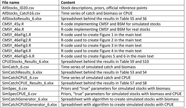
The subsequent appendices show the results from CMSY and BSM runs against 48 simulated stocks and 159 real stocks. The graphical output produced by the R-code for simulated data is shown in Figure 1 for a case of high-low-high biomass of a simulated stock with medium resilience. The six individual panels of the graph are explained below.
9
Figure 1. Example of the graphical CMSY-BSM output for a simulated stock with high-low-high biomass and medium resilience (HLH-M). See text for explanation of the panels.
The “HLH_M catch” panel indicates the name of the stock and shows the time series of catch data.
The red circles indicated the highest and the lowest catch, respectively, and the dashed green line indicates the “true” value of MSY used in the simulation.
The “Finding viable r-k” panel shows the analyzed log-r-k-space, with viable r-k pairs in dark gray and a green cross indicating the “true” r-k pair with approximate confidence limits based on process and observation error as assumed in the simulation. While CMSY is executed, this graph shows progress by adding dots as viable r-k pairs are found.
The “Analysis of viable r-k” panel shows the result of the CMSY-analysis, with viable pairs in gray and the predicted most probable r-k pair in blue, with approximate 95% confidence limits. The black dots are viable pairs identified by the Bayesian implementation of the full Schaefer model (BSM), with the red dot showing the predicted most probably r-k pair, with 95% confidence limits. The green dot shows the true values of r and k as used in the simulation. Good performance of CMSY and BSM is indicated by the green confidence limits overlapping with the blue (CMSY) and red (BSM) ones, respectively.
The “Pred. biomass vs observed” panel shows in blue the median biomass trajectory predicted by CMSY, with 2.5th and 97.5th percentiles as dotted black lines. The green curve shows the simulated
10
“true” biomass trajectory, scaled by the “true” value of k. The red curves indicate biomass scaled by the BSM estimate of k, with approximate 95% confidence limits as dotted red curves. The Y-axis gives biomass relative to k, so the broken line at 0.5 k indicates Bmsy and the dotted line at 0.25 k indicates the border to stock sizes that may result in reduced recruitment. The blue vertical lines show the prior biomass ranges set by the user or by prior rules. In the example of Figure 1, it was assumed that the user knew that the stock was in good status at the beginning and the end of the time series, and in bad status in-between, around year 25. Good performance of CMSY and BSM is indicated by the “true” green curve falling within the confidence limits of the black (CMSY) and the red (BSM) curves, respectively.
The “Exploitation rate” graph shows the time series of the catch/biomass ratio (u) relative to the ratio corresponding to MSY. The blue curve is the relative exploitation rate resulting from catch versus biomass predicted by CMSY. The red curve is the relative exploitation rate resulting from catch versus biomass scaled by the r-estimate of BSM. The “true” green curve relates simulated catch to simulated biomass. The dashed horizontal line indicates the maximum sustainable exploitation rate. Good performance of CMSY and BSM is indicated by close proximity of the blue and the red curves, respectively, to the “true” green curve.
The “Equilibrium curve” panel shows the Schaefer parabola with catch expressed relative to MSY on the Y-axis and decreasing biomass relative to k on the X-axis. The right side of the parabola is indented because below 0.25 k, a linear decline of surplus production due to reduced recruitment is assumed. Green dots show the “true” data points of simulated catch and biomass. Blue dots are predicted by the CMSY method and red dots are predicted by BSM. Dots falling on the parabola indicate catches that will maintain the respective biomass. Dots above the parabola will shrink future biomass; dots below the parabola allow future biomass to increase. Good performance of CMSY and BSM is indicated by the blue and red dots being close to the “true” green dots, respectively.
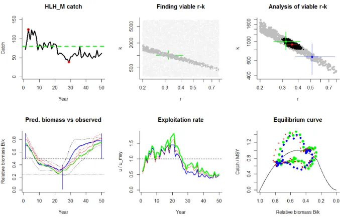
For real stocks, true parameter values are unknown and the parameter estimates of the Bayesian Schaefer model (BSM) are used instead as bench mark for CMSY. If observed biomass or CPUE are available, the graphical output looks as shown in Figure 2 for sole (Solea solea) in the Irish Sea. Note the better interpretation of yield at depleted biomass in Panel F, where the indented equilibrium curve suggests ongoing overfishing (red dots above curve). In this case CMSY still slightly
overestimates surplus production in the final years, due mostly to the too optimistic final biomass prior. That reduced recruitment is occurring in the final years is indicated by the declining biomass (red curve), despite the exploitation rate being below the MSY level.
11
Figure 2. R-code graphical output for stocks for which biomass or CPUE data are available. The thin blue line in Panel A indicates mean catches of the past three years.
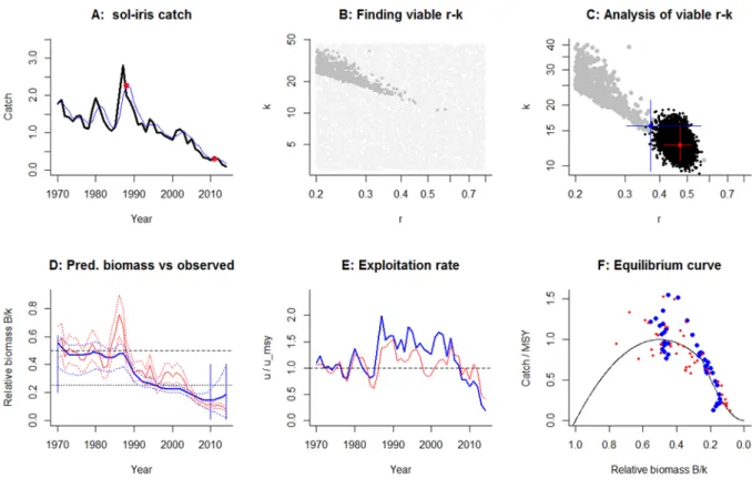
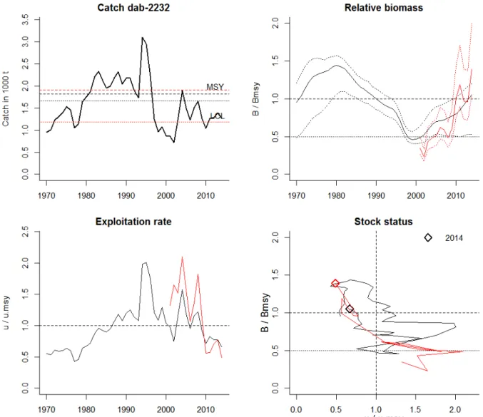
For data-limited stocks, an additional graphical output can be generated to support management decisions, as shown below for Baltic dab (Limanda limanda, dab-2232) (Figure 3).
12
Figure 3. Summary of information relevant for management of Baltic dab (dab-2232), with black curves indicating CMSY results and red curves BSM results. The horizontal dashed lines in the Catch graph indicate MSY and the fine dotted line indicates the lower confidence limit of MSY. The solid curves in the Relative biomass graph indicate predicted biomass relative to Bmsy, with confidence limits (dotted curves). Note that abundance time series data (here CPUE scaled to biomass, in red) can start later than the time series of catches. The Exploitation rate graph shows catch over predicted biomass (black curve) and catch over CPUE scaled by catchability q as estimated by BSM (red curve), with the dotted line indicating exploitation compatible with MSY. The Stock status graph shows the development of biomass and
exploitation relative to Bmsy (horizontal dashed line) and umsy (vertical dashed line), respectively. The fine dotted line indicates the biomass (0.5 Bmsy) below which recruitment may be impaired, and the rhomb indicates the final year in the time series.
In Appendix IV, the effect of analyzing landings instead of catches is explored with a simulated stock (07_HLH_M) and North Sea haddock (had-346a-land), a stock with very high rates of discards. The results can be compared with the respective analysis of catches for HLH_M in Appendix I and with had-346a in Appendix II in the ICES area.
13
Results
CMSY and BSM results compared with “true” values from simulated data
Catch and biomass data were simulated over a period of 50 years to create scenarios of heavily as well as lightly depleted stocks, with monotone stable or monotone changing biomass (i.e., steadily decreasing or increasing) or with alternating biomass trajectories: patterns of high-high (HH), high- low (HL), high-low-high (HLH), low-low (LL), low-high (LH), and low-high-low (LHL) biomass trends.
Simulated stocks have names that indicate the combination of biomass trajectory and intrinsic growth rate (High, Medium, Low, Very Low), e.g., HH_L signifies a stock with monotone high biomass and low resilience. See Material and Methods and main text for further description of the
simulations. The “true” parameter values of the Schaefer model used in the simulations to generate the time series of biomass given the catches were k = 1,000,000 in all cases, and r drawn randomly from a normal distribution within the ranges associated with the resilience classes (Table S2). Table S3 shows the CMSY estimates of MSY, r, k, and biomass in the last year compared with the “true”
values from the simulations. True values were not included in the confidence limits in eight of the 24 simulated stocks.
14
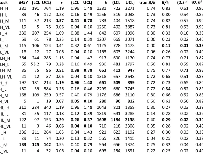
Table S3. Results of estimating the parameters of the Schaefer model with the CMSY method, for 24 simulated stocks.
LCL and UCL indicate the lower and upper 95% confidence limits, respectively. Cases where the confidence limits do not include the “true” parameter values are indicated in bold. [SimCatchResults_6.xlsx]
Stock MSY (LCL UCL) r (LCL UCL) k (LCL UCL) true B/k B/k (2.5th 97.5th) HH_H 381 191 764 1.19 0.96 1.48 1281 722 2271 0.74 0.83 0.61 0.90 HH_L 89 46 172 0.28 0.16 0.49 1256 519 3038 0.73 0.80 0.54 0.89 HH_M 111 57 213 0.57 0.41 0.78 783 404 1518 0.74 0.82 0.57 0.90 HH_VL 19 5 75 0.06 0.04 0.10 1250 402 3887 0.73 0.81 0.53 0.90 HL_H 230 207 254 1.09 0.88 1.44 842 607 1096 0.30 0.33 0.10 0.39 HL_L 69 61 78 0.23 0.14 0.39 1207 669 2071 0.06 0.23 0.02 0.40 HL_M 115 106 124 0.41 0.32 0.61 1125 728 1473 0.00 0.11 0.01 0.38 HL_VL 18 12 27 0.06 0.04 0.10 1163 603 2244 0.06 0.26 0.02 0.40 HLH_H 264 244 285 1.15 0.94 1.47 917 690 1170 0.74 0.77 0.71 0.82 HLH_L 65 53.2 79 0.28 0.16 0.49 930 481 1797 0.66 0.81 0.59 0.87 HLH_M 85 75 96 0.51 0.38 0.78 662 411 947 0.75 0.77 0.71 0.82 HLH_VL 21 12 37 0.06 0.04 0.10 1318 657 2648 0.72 0.65 0.51 0.83 LH_H 197 181 214 1.19 0.96 1.48 661 509 859 0.72 0.73 0.65 0.80 LH_L 150 39 584 0.26 0.16 0.46 2299 660 7745 0.72 0.84 0.52 0.89 LH_M 168 109 259 0.57 0.40 0.79 1176 686 2110 0.80 0.66 0.52 0.83
LH_VL 5 1 19 0.07 0.05 0.10 280 96 812 0.60 0.62 0.50 0.82
LHL_H 311 284 340 1.19 0.96 1.48 1043 801 1358 0.30 0.27 0.03 0.39 LHL_L 81 55 117 0.18 0.12 0.39 1819 691 3285 0.14 0.28 0.02 0.39 LHL_M 122 97 153 0.29 0.26 0.37 1698 1184 2138 0.40 0.29 0.02 0.39 LHL_VL 11 3 46 0.06 0.04 0.10 710 218 2308 0.35 0.28 0.02 0.40 LL_H 236 211 264 1.03 0.84 1.43 921 623 1192 0.27 0.30 0.03 0.39 LL_L 29 11 74 0.20 0.13 0.32 565 226 1415 0.04 0.25 0.02 0.39 LL_M 133 125 142 0.55 0.40 0.79 964 656 1374 0.25 0.32 0.04 0.40 LL_VL 11 4 32 0.06 0.04 0.10 693 254 1891 0.22 0.25 0.02 0.40
15
Table S4 shows the BSM estimates of r, k, and MSY compared with the “true” values from the simulations. True values of eight simulated stocks were not included in the respective BSM
confidence limits. Five of the “missed” stocks were identical with the ones where also CMSY did not include all of the “true” values in its respective confidence limits.
Table S4. Results of estimating the parameters of the Schaefer model with the BSM method, for 24 simulated stocks. LCL and UCL indicate the lower and upper 95% confidence limits, respectively. The cases where the confidence limits do not include the “true” parameter value are indicated in bold. [SimCatchResults_6.xlsx]
Stock MSY (LCL UCL) r (LCL UCL) k (LCL UCL) HH_H 266 253 283 1.05 0.97 1.15 1009 976 1046 HH_L 69 61 77 0.27 0.23 0.32 1010 952 1090 HH_M 113 102 125 0.50 0.43 0.57 909 881 943 HH_VL 13 7 18 0.05 0.02 0.08 1022 877 1274 HL_H 225 217 234 0.94 0.88 1.01 955 900 1010 HL_L 73 68 79 0.29 0.27 0.31 995 923 1072
HL_M 77 64 95 0.50 0.45 0.58 611 522 718
HL_VL 18 14 23 0.07 0.06 0.08 1055 894 1202 HLH_H 259 248 272 1.06 1.02 1.13 973 914 1030 HLH_L 60 54 66 0.24 0.23 0.27 981 890 1082 HLH_M 82 78 88 0.36 0.33 0.39 920 851 1015 HLH_VL 19 15 24 0.07 0.06 0.09 1052 900 1197 LH_H 205 196 216 0.88 0.824 0.94 934 890 980 LH_L 62 54 299 0.25 0.22 0.29 991 885 4314 LH_M 165 156 173 0.66 0.61 0.70 997 949 1056 LH_VL 10 7 16 0.05 0.03 0.06 906 568 1424 LHL_H 296 282 312 1.11 1.04 1.21 1065 971 1171 LHL_L 84 78 90 0.35 0.33 0.37 946 897 1006 LHL_M 129 119 140 0.54 0.51 0.58 955 884 1033 LHL_VL 36 13 68 0.04 0.02 0.06 3308 1883 4608 LL_H 230 211 258 1.04 0.94 1.12 884 780 1073 LL_L 91 46 129 0.27 0.21 0.32 1325 900 1632 LL_M 144 129 162 0.60 0.56 0.64 961 843 1093 LL_VL 12 8 59 0.07 0.05 0.13 771 610 1797
16
Comparison of CMSY and BSM parameter estimates for 128 fully assessed stocks
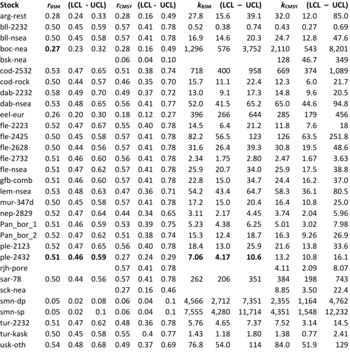
Table S5 shows a comparison of CMSY parameter estimates of r and k with those derived from a full Schaefer model (BSM). Significant deviations in estimates of r occurred in 14 of the 128 stocks (11%).
Significant deviations in the estimates k occurred in 20 stocks (16%). These cases are marked bold.
Table S6 shows a comparison of CMSY and BSM estimates of MSY. Significant deviations occurred in 6 of the 128 stocks (5%). Table S6 also shows a comparison of last year’s observed biomass relative to k estimated by BSM and observed exploitation rate (catch/biomass) and compares these observations with the respective CMSY estimates. The relative biomass estimate was significantly different in 13 of the stocks (10%) and the BSM exploitation rate relative to the MSY level differed more than +/-50% from the CMSY estimate in 40 stocks (31%).
17
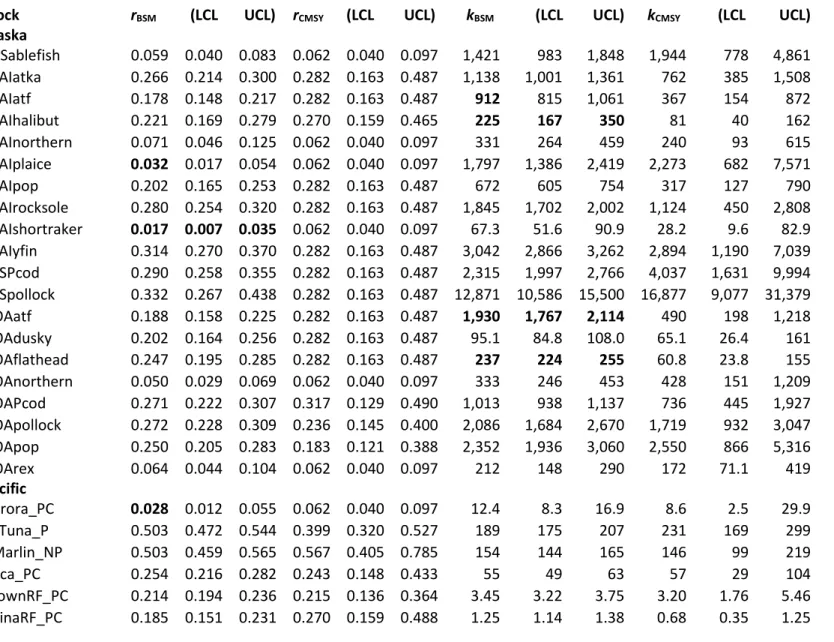
Table S5. Comparison of estimates of r and k by CMSY and BSM fitted to 112 real stocks, where LCL and UCL indicate lower and upper 95% confidence limits, respectively.
Cases where the BSM estimate is not included in the CMSY confidence limits are marked in bold. Similarly, cases where the confidence limits of both methods do not overlap are marked in bold. [AllStocks_Results_6.xlsx]
Stock rBSM (LCL UCL) rCMSY (LCL UCL) kBSM (LCL UCL) kCMSY (LCL UCL) Alaska
AKSablefish 0.059 0.040 0.083 0.062 0.040 0.097 1,421 983 1,848 1,944 778 4,861 BSAIatka 0.266 0.214 0.300 0.282 0.163 0.487 1,138 1,001 1,361 762 385 1,508 BSAIatf 0.178 0.148 0.217 0.282 0.163 0.487 912 815 1,061 367 154 872 BSAIhalibut 0.221 0.169 0.279 0.270 0.159 0.465 225 167 350 81 40 162 BSAInorthern 0.071 0.046 0.125 0.062 0.040 0.097 331 264 459 240 93 615 BSAIplaice 0.032 0.017 0.054 0.062 0.040 0.097 1,797 1,386 2,419 2,273 682 7,571
BSAIpop 0.202 0.165 0.253 0.282 0.163 0.487 672 605 754 317 127 790
BSAIrocksole 0.280 0.254 0.320 0.282 0.163 0.487 1,845 1,702 2,002 1,124 450 2,808 BSAIshortraker 0.017 0.007 0.035 0.062 0.040 0.097 67.3 51.6 90.9 28.2 9.6 82.9 BSAIyfin 0.314 0.270 0.370 0.282 0.163 0.487 3,042 2,866 3,262 2,894 1,190 7,039 EBSPcod 0.290 0.258 0.355 0.282 0.163 0.487 2,315 1,997 2,766 4,037 1,631 9,994 EBSpollock 0.332 0.267 0.438 0.282 0.163 0.487 12,871 10,586 15,500 16,877 9,077 31,379 GOAatf 0.188 0.158 0.225 0.282 0.163 0.487 1,930 1,767 2,114 490 198 1,218 GOAdusky 0.202 0.164 0.256 0.282 0.163 0.487 95.1 84.8 108.0 65.1 26.4 161 GOAflathead 0.247 0.195 0.285 0.282 0.163 0.487 237 224 255 60.8 23.8 155 GOAnorthern 0.050 0.029 0.069 0.062 0.040 0.097 333 246 453 428 151 1,209 GOAPcod 0.271 0.222 0.307 0.317 0.129 0.490 1,013 938 1,137 736 445 1,927 GOApollock 0.272 0.228 0.309 0.236 0.145 0.400 2,086 1,684 2,670 1,719 932 3,047 GOApop 0.250 0.205 0.283 0.183 0.121 0.388 2,352 1,936 3,060 2,550 866 5,316
GOArex 0.064 0.044 0.104 0.062 0.040 0.097 212 148 290 172 71.1 419
Pacific
Aurora_PC 0.028 0.012 0.055 0.062 0.040 0.097 12.4 8.3 16.9 8.6 2.5 29.9
BFTuna_P 0.503 0.472 0.544 0.399 0.320 0.527 189 175 207 231 169 299
BMarlin_NP 0.503 0.459 0.565 0.567 0.405 0.785 154 144 165 146 99 219
Boca_PC 0.254 0.216 0.282 0.243 0.148 0.433 55 49 63 57 29 104
BrownRF_PC 0.214 0.194 0.236 0.215 0.136 0.364 3.45 3.22 3.75 3.20 1.76 5.46 ChinaRF_PC 0.185 0.151 0.231 0.270 0.159 0.488 1.25 1.14 1.38 0.68 0.35 1.25
18
Stock rBSM (LCL UCL) rCMSY (LCL UCL) kBSM (LCL UCL) kCMSY (LCL UCL) CopperRF_PC 0.184 0.163 0.208 0.200 0.129 0.340 5.35 4.97 5.77 4.41 2.37 7.47 Cowcod_PC 0.275 0.241 0.314 0.254 0.152 0.469 2.05 1.74 2.70 2.00 0.97 3.74 DarkblotchedRF_PC 0.093 0.065 0.118 0.062 0.040 0.097 37.9 33.0 45.7 37.6 20.4 69.6 LongspinTH_PC 0.059 0.043 0.083 0.062 0.040 0.097 184 138 241 114 64 203 PetraleSole_PC 0.446 0.416 0.481 0.381 0.311 0.503 23.8 22.1 25.8 27.1 19.8 34.5 Phake_PC 0.495 0.428 0.547 0.566 0.407 0.785 3,340 2,818 4,213 1,945 1,293 2,926 Rougheye_PC 0.035 0.019 0.054 0.062 0.040 0.097 29.4 21.1 38.3 23.5 8.5 64.6 Sardine_P 0.501 0.443 0.567 0.566 0.407 0.785 1,409 1,247 1,626 946 598 1,495 ShortspinTH_PC 0.016 0.007 0.033 0.062 0.040 0.097 589 422 851 164 69 394 Northwest Atlantic
Ahalibut_NWAC 0.270 0.248 0.287 0.254 0.152 0.448 2.17 1.95 2.41 2.28 1.20 4.12 Albacore_NA 0.376 0.338 0.425 0.346 0.289 0.413 451 417 487 497 406 610
BETuna_A 0.451 0.424 0.480 0.568 0.411 0.785 850 831 870 661 451 968
Bluefish_AC 0.474 0.402 0.524 0.399 0.320 0.542 209 160 350 451 222 840
BSbass_MAC 0.522 0.481 0.599 0.564 0.409 0.785 23 20 26 21 14 30
Cod_GB 0.517 0.473 0.596 0.387 0.314 0.592 202 167 266 363 182 586
Cod_GUM 0.694 0.570 0.799 0.413 0.329 0.672 61 52 77 147 67 248
Haddock_GB 0.310 0.263 0.407 0.183 0.122 0.288 417 317 607 1,137 507 2,423 Haddock_GoM 0.500 0.436 0.568 0.407 0.325 0.656 23.8 15.8 77.0 30.7 17.3 42.3 Herring_A 0.520 0.473 0.611 0.533 0.391 0.743 1,687 1,470 2,004 1,901 1,263 2,794 Swordfish_NA 0.449 0.423 0.477 0.573 0.422 0.778 127 123 131 97 69 137 Whake_GUMGB 0.396 0.351 0.437 0.262 0.155 0.475 46.2 42.2 51.8 70.2 34.6 133
YTFlo_MA 0.506 0.453 0.597 0.436 0.341 0.573 107 43 230 97 54 171
Caribbean
GAGGM 0.512 0.470 0.594 0.309 0.268 0.356 18.0 14.8 21.8 29.9 24.4 36.7 RGROUPGM 0.767 0.633 0.885 0.375 0.307 0.500 5.48 4.65 6.69 17 8.68 31.2 VSNAPSATLC 0.220 0.177 0.274 0.282 0.163 0.487 8.84 7.83 10.2 4.95 2.54 9.6 Mediterranean
Encr_engr_GSA17 0.493 0.429 0.538 0.561 0.405 0.777 312 259 404 235 160 345 mul-gsa6 0.537 0.491 0.621 0.566 0.407 0.785 9.8 7.7 11.6 8.6 5.5 13.5 mullsur_gsa1516 1.067 1.009 1.189 1.165 0.943 1.453 7.0 5.7 8.1 7.0 4.6 10.5
19
Stock rBSM (LCL UCL) rCMSY (LCL UCL) kBSM (LCL UCL) kCMSY (LCL UCL) Black Sea
BS_anch 0.501 0.447 0.575 0.566 0.407 0.785 3,550 2,802 4,678 2,454 1,617 3,724
Spr_BS 0.502 0.449 0.568 0.566 0.407 0.785 577 493 694 616 308 1,231
Tur_BS 0.498 0.459 0.534 0.309 0.268 0.356 23.8 21.4 26.7 40.3 32.3 50.4 South Africa
CRPN_S 0.227 0.170 0.280 0.278 0.162 0.487 6.2 5.3 9.0 6.2 1.9 19.4
CRPN_SE 0.215 0.177 0.264 0.282 0.163 0.487 10.1 8.6 12.8 8.4 2.7 26.7
HTTN_SW 0.479 0.389 0.531 0.266 0.242 0.292 1.5 1.3 1.8 2.8 2.4 3.2
HTTN_W 0.480 0.391 0.531 0.276 0.248 0.307 4.0 3.7 4.8 6.0 5.1 7.0
KKLI_S 0.170 0.143 0.203 0.278 0.162 0.478 54.5 50.4 59.7 29.2 15.2 56.0
KOB_S 0.343 0.303 0.403 0.278 0.162 0.478 6.9 5.4 8.1 9.5 4.0 22.2
KOB_SE 0.356 0.307 0.416 0.274 0.160 0.468 3.6 2.9 4.4 5.0 2.1 11.6
SLNG 0.494 0.439 0.533 0.541 0.395 0.773 1.9 1.7 2.2 1.5 1.0 2.3
SA-BSH 0.307 0.261 0.388 0.287 0.114 0.482 274 240 324 267 136 779
Northeast Atlantic
anp-8c9a 0.703 0.580 0.822 0.359 0.298 0.544 20.5 17.8 24.7 59.0 30.6 90.2 Bss-47 0.259 0.211 0.292 0.282 0.163 0.487 40.9 32.7 53.8 38.2 19.3 75.7
cod-2224 0.859 0.702 0.989 0.346 0.289 0.413 214 180 263 626 474 825
cod-347d 0.519 0.477 0.603 0.359 0.297 0.434 1,653 1,371 2,121 2,944 2,222 3,899 cod-7e-k 0.616 0.514 0.714 0.462 0.355 0.731 52.2 43.0 64.9 83.4 50.3 114 cod-arct 0.608 0.541 0.674 0.455 0.351 0.650 4,813 4,326 5,454 6,583 4,441 8,845
cod-farp 0.528 0.481 0.613 0.417 0.330 0.607 172 149 203 244 160 323
cod-iceg 0.510 0.480 0.560 0.333 0.282 0.464 2,783 2,408 3,276 4,330 2,985 5,325
cod-scow 0.509 0.464 0.593 0.436 0.341 0.621 114 83 165 212 103 392
dgs-nea 0.106 0.088 0.132 0.183 0.122 0.290 1,740 1,463 2,095 804 470 1,299 ghl-arct 0.315 0.272 0.365 0.236 0.145 0.431 417 342 509 654 267 1,427 had-346a 0.494 0.427 0.545 0.318 0.275 0.385 2,113 1,690 2,934 2,778 2,106 3,505
had-7b-k 0.505 0.458 0.584 0.399 0.320 0.500 111 89 151 179 130 244
had-arct 0.542 0.486 0.639 0.472 0.360 0.699 1,091 946 1,285 1,337 843 1,876
had-faro 0.493 0.429 0.540 0.387 0.312 0.479 146 126 170 180 137 236
had-iceg 0.606 0.523 0.682 0.566 0.407 0.785 405 359 465 513 329 799
20
Stock rBSM (LCL UCL) rCMSY (LCL UCL) kBSM (LCL UCL) kCMSY (LCL UCL)
had-rock 0.497 0.434 0.556 0.494 0.372 0.779 99 72 157 140 64 259
her-2532-gor 0.361 0.306 0.438 0.364 0.301 0.571 2,839 2,456 3,324 2,529 1,519 3,247
her-30 0.410 0.342 0.497 0.566 0.407 0.785 862 754 994 470 320 689
her-3a22 0.523 0.489 0.571 0.455 0.351 0.717 1,036 891 1,187 1,647 708 3,148 her-47d3 0.485 0.416 0.526 0.463 0.349 0.732 6,369 5,763 7,265 5,592 3,376 7,762 her-67bc 0.390 0.329 0.471 0.297 0.261 0.339 1,302 1,177 1,463 1,375 1,115 1,695
her-irls 0.462 0.384 0.515 0.387 0.312 0.479 249 218 301 212 165 272
her-nirs 0.422 0.369 0.490 0.321 0.275 0.393 123 105 145 182 135 234
her-noss 0.475 0.400 0.523 0.566 0.407 0.785 11,174 10,180 12,366 7,654 4,922 11,904
her-riga 0.495 0.437 0.542 0.566 0.407 0.785 232 205 270 221 148 331
her-vian 0.432 0.360 0.503 0.333 0.282 0.410 938 786 1,158 1,103 832 1,404 hke-nrtn 0.906 0.733 1.039 0.566 0.407 0.785 278 247 315 715 383 1,333
hke-soth 0.884 0.663 1.053 0.465 0.357 0.725 64 55 75 134 78 193
hom-west 0.447 0.368 0.511 0.498 0.373 0.752 4,013 3,438 4,927 2,395 1,486 3,409
lin-icel 0.510 0.482 0.551 0.566 0.407 0.785 129 115 142 99 49 198
mac-nea 0.438 0.367 0.504 0.566 0.407 0.785 7,017 6,248 8,400 6,724 3,719 12,157 mgw-8c9a 0.315 0.268 0.377 0.262 0.155 0.465 6.40 5.09 8.20 11 4.03 26 nep-8ab 0.507 0.476 0.566 0.546 0.395 0.785 44.3 37.9 50.6 39.9 26.1 58.8 nop-34-june 0.498 0.436 0.552 0.430 0.337 0.605 1,909 1,367 2,780 3,714 1,673 7,462 ple-celt 0.525 0.485 0.587 0.525 0.387 0.763 2.23 1.85 2.62 3.04 1.48 5.82 ple-eche 0.589 0.503 0.673 0.537 0.393 0.742 31.4 26.4 37.7 36.6 24.9 53.2 ple-echw 0.500 0.460 0.550 0.498 0.373 0.705 14.8 12.6 17.3 15.3 10.1 21.8 ple-nsea 0.578 0.530 0.635 0.309 0.268 0.356 1,325 1,153 1,480 2,873 2,282 3,618 sai-3a46 0.504 0.468 0.557 0.313 0.269 0.392 1,253 1,081 1,471 2,395 1,667 3,208 sai-arct 0.551 0.503 0.599 0.529 0.389 0.778 1,280 1,188 1,391 1,353 882 1,916
sai-faro 0.493 0.438 0.534 0.566 0.407 0.785 344 314 385 320 213 480
sai-icel 0.477 0.414 0.522 0.533 0.391 0.770 550 478 665 503 323 738
san-ns1 1.056 0.984 1.169 0.995 0.829 1.420 1,406 1,264 1,593 1,482 967 1,910
san-ns2 1.042 0.940 1.121 0.896 0.755 1.019 434 380 494 380 309 488
san-ns3 1.050 0.978 1.134 1.049 0.851 1.380 1,210 1,114 1,307 1,262 890 1,675 sar-soth 0.509 0.465 0.591 0.399 0.320 0.565 1,028 842 1,275 1,673 980 2,505
21
Stock rBSM (LCL UCL) rCMSY (LCL UCL) kBSM (LCL UCL) kCMSY (LCL UCL) smn-con 0.273 0.236 0.308 0.282 0.163 0.487 307 241 411 420 156 1,134 sol-bisc 0.507 0.466 0.576 0.546 0.395 0.785 42.5 35.6 50.7 40.6 26.3 60.3 sol-celt 0.487 0.421 0.531 0.505 0.377 0.712 9.7 8.5 11.8 9.4 6.3 13.3 sol-eche 0.517 0.476 0.600 0.566 0.407 0.785 33.5 28.8 39.4 31.6 21.0 47.5 sol-echw 0.479 0.413 0.522 0.537 0.393 0.773 8.6 7.8 10.0 8.0 5.4 11.5 sol-iris 0.473 0.412 0.516 0.370 0.304 0.559 12.6 10.6 15.8 15.8 9.4 21.3
sol-kask 0.505 0.460 0.580 0.517 0.383 0.758 6.1 5.3 7.2 6.6 4.2 9.4
sol-nsea 0.507 0.472 0.568 0.456 0.349 0.673 198 168 235 227 148 309
spr-2232 0.490 0.417 0.537 0.561 0.405 0.777 2,756 2,296 3,593 2,466 1,650 3,684 spr-nsea 0.499 0.438 0.563 0.456 0.351 0.637 3,787 2,082 9,737 2,794 1,739 4,177
usk-icel 0.330 0.299 0.372 0.385 0.301 0.493 85 70 100 65 49 88
whb-comb 0.465 0.398 0.515 0.557 0.403 0.785 10,973 9,227 13,398 9,833 6,425 14,751 whg-47d 0.494 0.425 0.549 0.452 0.349 0.664 930 776 1,162 699 424 1,012
whg-7e-k 0.565 0.494 0.661 0.566 0.407 0.785 101 87 123 109 73 161
whg-scow 0.491 0.419 0.538 0.458 0.351 0.685 126 101 167 116 73 163
22
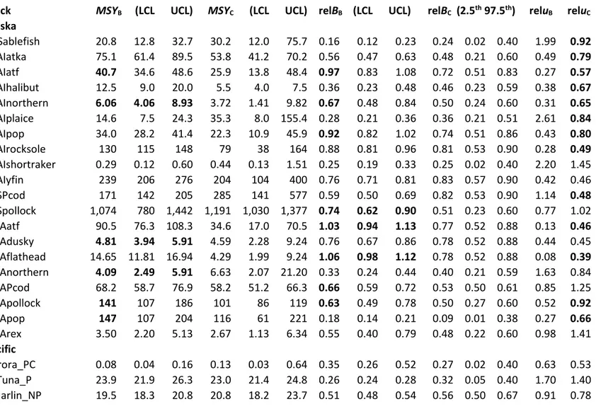
Table S6. Comparison of parameter estimates of CMSY and BSM fitted to 128 real stocks, where subscript B stands for estimates by BSM and subscript C stands for estimates by CMSY. relB is the B/k ratio and relu is the relative exploitation rate (u/umsy) in the last year. LCL and UCL indicate lower and upper 95% confidence limits, respectively.
Cases where the BSM estimate of MSY or observed B/k are not included in the CMSY confidence limits or percentile range are marked in bold. Similarly, cases where the confidence limits do not overlap are marked in bold. Cases where the last relative exploitation rate estimated by CMSY (reluC) differs more than 50% from the observed rate are marked bold. [AllStocks_Results_6.xlsx]
Stock MSYB (LCL UCL) MSYC (LCL UCL) relBB (LCL UCL) relBC (2.5th 97.5th)
reluB reluC
Alaska
AKSablefish 20.8 12.8 32.7 30.2 12.0 75.7 0.16 0.12 0.23 0.24 0.02 0.40 1.99 0.92 BSAIatka 75.1 61.4 89.5 53.8 41.2 70.2 0.56 0.47 0.63 0.48 0.21 0.60 0.49 0.79 BSAIatf 40.7 34.6 48.6 25.9 13.8 48.4 0.97 0.83 1.08 0.72 0.51 0.83 0.27 0.57 BSAIhalibut 12.5 9.0 20.0 5.5 4.0 7.5 0.36 0.23 0.48 0.46 0.23 0.59 0.38 0.67 BSAInorthern 6.06 4.06 8.93 3.72 1.41 9.82 0.67 0.48 0.84 0.50 0.24 0.60 0.31 0.65 BSAIplaice 14.6 7.5 24.3 35.3 8.0 155.4 0.28 0.21 0.36 0.36 0.21 0.51 2.61 0.84 BSAIpop 34.0 28.2 41.4 22.3 10.9 45.9 0.92 0.82 1.02 0.74 0.51 0.86 0.43 0.80 BSAIrocksole 130 115 148 79 38 164 0.88 0.81 0.96 0.81 0.53 0.90 0.28 0.49 BSAIshortraker 0.29 0.12 0.60 0.44 0.13 1.51 0.25 0.19 0.33 0.25 0.02 0.40 2.20 1.45 BSAIyfin 239 206 276 204 104 400 0.76 0.71 0.81 0.83 0.57 0.90 0.42 0.46 EBSPcod 171 142 205 285 141 577 0.59 0.50 0.69 0.82 0.53 0.90 1.14 0.48 EBSpollock 1,074 780 1,442 1,191 1,030 1,377 0.74 0.62 0.90 0.51 0.23 0.60 0.77 1.02 GOAatf 90.5 76.3 108.3 34.6 17.0 70.5 1.03 0.94 1.13 0.77 0.52 0.88 0.13 0.46 GOAdusky 4.81 3.94 5.91 4.59 2.28 9.24 0.76 0.67 0.86 0.78 0.52 0.88 0.44 0.45 GOAflathead 14.65 11.81 16.94 4.29 1.99 9.24 1.06 0.98 1.12 0.78 0.52 0.88 0.08 0.39 GOAnorthern 4.09 2.49 5.91 6.63 2.07 21.20 0.33 0.24 0.44 0.40 0.21 0.59 1.63 0.84 GOAPcod 68.2 58.7 76.9 58.2 51.2 66.3 0.66 0.59 0.72 0.53 0.50 0.61 0.85 1.25 GOApollock 141 107 186 101 86 119 0.63 0.49 0.78 0.50 0.27 0.60 0.52 0.92
GOApop 147 107 204 116 61 221 0.18 0.14 0.21 0.09 0.01 0.38 0.27 0.66
GOArex 3.50 2.20 5.13 2.67 1.13 6.34 0.55 0.40 0.79 0.48 0.22 0.60 0.98 1.41
Pacific
Aurora_PC 0.08 0.04 0.16 0.13 0.03 0.64 0.35 0.26 0.52 0.27 0.02 0.40 0.63 0.53 BFTuna_P 23.9 21.9 26.3 23.0 21.4 24.8 0.26 0.24 0.28 0.32 0.05 0.40 1.70 1.40 BMarlin_NP 19.5 18.3 20.8 20.8 18.2 23.7 0.51 0.48 0.54 0.56 0.50 0.67 0.91 0.78
23
Stock MSYB (LCL UCL) MSYC (LCL UCL) relBB (LCL UCL) relBC (2.5th 97.5th)
reluB reluC Boca_PC 3.50 2.91 4.11 3.45 2.80 4.26 0.30 0.26 0.33 0.11 0.01 0.38 0.06 0.17 BrownRF_PC 0.18 0.17 0.20 0.17 0.15 0.20 0.41 0.37 0.44 0.51 0.27 0.60 0.68 0.57 ChinaRF_PC 0.06 0.05 0.07 0.05 0.04 0.05 0.62 0.56 0.68 0.47 0.24 0.59 0.44 0.73 CopperRF_PC 0.25 0.22 0.27 0.22 0.18 0.26 0.61 0.56 0.65 0.52 0.24 0.60 0.26 0.34 Cowcod_PC 0.14 0.12 0.18 0.13 0.10 0.16 0.50 0.38 0.58 0.42 0.21 0.59 0.00 0.01 DarkblotchedRF_PC 0.88 0.66 1.10 0.58 0.42 0.81 0.41 0.343 0.48 0.25 0.02 0.40 0.26 0.64 LongspinTH_PC 2.76 1.96 3.80 1.77 1.38 2.28 0.37 0.283 0.49 0.35 0.17 0.40 0.57 0.93 PetraleSole_PC 2.65 2.49 2.84 2.59 2.40 2.78 0.63 0.582 0.68 0.53 0.29 0.60 0.29 0.34 Phake_PC 411 334 517 275 235 322 0.65 0.512 0.77 0.51 0.26 0.60 0.45 0.84 Rougheye_PC 0.25 0.14 0.40 0.36 0.12 1.10 0.29 0.222 0.4 0.26 0.02 0.40 1.40 1.09 Sardine_P 177 151 207 134 104 173 0.54 0.467 0.61 0.49 0.26 0.60 0.74 1.06 ShortspinTH_PC 2.39 1.02 4.50 2.55 1.10 5.90 0.40 0.287 0.58 0.25 0.02 0.40 0.60 0.86
Northwest Atlantic
Ahalibut_NWAC 0.15 0.13 0.16 0.14 0.12 0.17 0.77 0.69 0.85 0.72 0.53 0.85 0.37 0.40 Albacore_NA 42.5 38.7 46.9 43.0 40.9 45.1 0.41 0.38 0.45 0.29 0.02 0.40 0.52 0.72 BETuna_A 95.7 90.9 100.9 93.9 83.6 105.4 0.50 0.49 0.51 0.42 0.22 0.59 0.83 1.01 Bluefish_AC 24.6 19.5 41.2 44.9 20.4 99.1 0.39 0.23 0.51 0.18 0.01 0.39 0.55 0.65 BSbass_MAC 3.05 2.72 3.42 2.89 2.64 3.17 0.55 0.48 0.62 0.50 0.25 0.60 0.61 0.69 Cod_GB 26.5 21.3 34.9 35.1 20.7 59.5 0.14 0.11 0.17 0.11 0.02 0.38 0.46 0.43 Cod_GUM 10.6 8.3 13.8 15.1 8.4 27.1 0.24 0.19 0.28 0.20 0.01 0.40 1.49 1.25 Haddock_GB 33.1 23.4 49.2 51.9 26.0 103.7 0.45 0.31 0.59 0.46 0.22 0.60 0.81 0.49 Haddock_GoM 3.04 1.97 9.54 3.12 2.58 3.77 0.15 0.05 0.23 0.21 0.02 0.39 1.27 0.88 Herring_A 223 188 269 253 218 294 0.78 0.66 0.90 0.88 0.85 0.90 0.26 0.20 Swordfish_NA 14.3 13.6 15.0 13.8 12.8 14.9 0.58 0.56 0.60 0.48 0.24 0.59 0.73 0.91 Whake_GUMGB 4.58 4.11 5.05 4.60 3.69 5.73 0.68 0.60 0.739 0.51 0.25 0.60 0.35 0.46 YTFlo_MA 13.7 5.5 29.1 10.6 5.7 19.7 0.05 0.02 0.12 0.12 0.01 0.38 0.28 0.15
Caribbean/Gulf of Mexico
GAGGM 2.33 1.95 2.81 2.31 2.05 2.60 0.62 0.51 0.75 0.12 0.02 0.36 0.34 1.71 RGROUPGM 1.06 0.84 1.27 1.61 0.74 3.51 0.55 0.45 0.64 0.53 0.26 0.60 1.02 0.69 VSNAPSATLC 0.49 0.40 0.60 0.35 0.28 0.44 0.34 0.29 0.38 0.27 0.02 0.40 1.36 2.39
24
Stock MSYB (LCL UCL) MSYC (LCL UCL) relBB (LCL UCL) relBC (2.5th 97.5th)
reluB reluC
Mediterranean
Encr_engr_GSA17 38.3 31.5 49.4 33.0 29.5 36.9 0.71 0.55 0.85 0.53 0.50 0.60 0.77 1.20 mul-gsa6 1.31 1.13 1.50 1.22 0.96 1.55 0.30 0.25 0.38 0.28 0.03 0.40 1.45 1.65 mullsur_gsa1516 1.87 1.56 2.15 2.04 1.41 2.95 0.42 0.36 0.51 0.25 0.02 0.40 0.64 0.98
Black Sea
BS_anch 447 337 611 347 291 413 0.19 0.14 0.24 0.25 0.03 0.39 1.68 1.64 Spr_BS 72.8 60.3 88.4 87.0 42.6 178.0 0.72 0.60 0.84 0.75 0.51 0.86 0.97 0.77 Tur_BS 2.96 2.62 3.34 3.11 2.66 3.64 0.07 0.06 0.08 0.33 0.03 0.39 3.11 0.60
South Africa
CRPN_S 0.36 0.29 0.44 0.43 0.13 1.40 0.97 0.665 1.14 0.87 0.77 0.9 0.149 0.13 CRPN_SE 0.55 0.46 0.65 0.59 0.18 1.95 0.90 0.728 1.09 0.83 0.55 0.9 0.2 0.21 HTTN_SW 0.17 0.15 0.21 0.18 0.16 0.21 0.83 0.679 0.95 0.9 0.88 0.9 0.191 0.17 HTTN_W 0.48 0.41 0.56 0.41 0.37 0.46 0.95 0.803 1.06 0.89 0.88 0.9 0.134 0.17 KKLI_S 2.32 2.00 2.71 2.03 1.64 2.51 0.49 0.449 0.53 0.49 0.23 0.6 0.517 0.59 KOB_S 0.59 0.52 0.67 0.66 0.36 1.22 0.47 0.403 0.60 0.40 0.22 0.57 0.793 0.84 KOB_SE 0.32 0.27 0.37 0.34 0.18 0.63 0.50 0.418 0.64 0.43 0.22 0.58 0.604 0.67 SLNG 0.24 0.22 0.26 0.21 0.17 0.25 0.80 0.697 0.88 0.51 0.25 0.59 0.508 0.92 SA-BSH 21.4 18.6 24.5 19.1 14.2 25.7 0.53 0.451 0.61 0.24 0.20 0.36 1.284 3.14
Northeast Atlantic
anp-8c9a 3.62 2.90 4.38 5.29 3.31 8.47 0.46 0.38 0.53 0.49 0.23 0.60 0.50 0.31 Bss-47 2.62 2.10 3.32 2.70 2.07 3.52 0.28 0.21 0.35 0.29 0.03 0.40 2.44 2.33 cod-2224 45.1 34.7 61.5 54.0 44.6 65.5 0.19 0.16 0.23 0.16 0.02 0.39 1.08 1.08 cod-347d 218 176 277 264 221 316 0.20 0.16 0.24 0.12 0.01 0.38 0.50 0.70 cod-7e-k 8.01 6.37 10.04 9.63 8.80 10.53 0.23 0.19 0.28 0.25 0.03 0.40 1.79 1.39 cod-arct 732 644 827 749 697 804 0.65 0.58 0.73 0.69 0.60 0.74 0.93 0.86 cod-farp 22.9 19.3 27.7 25.5 23.2 27.9 0.16 0.14 0.19 0.15 0.02 0.39 0.83 0.79 cod-iceg 356 314 415 360 333 390 0.42 0.36 0.49 0.52 0.21 0.59 0.71 0.57 cod-scow 14.7 10.6 21.8 23.1 11.2 47.6 0.04 0.03 0.06 0.10 0.01 0.37 1.35 0.36 dgs-nea 46.3 36.2 60.7 36.7 31.7 42.6 0.13 0.11 0.15 0.17 0.01 0.39 0.20 0.19 ghl-arct 32.8 25.6 42.1 38.5 21.7 68.2 0.74 0.61 0.90 0.74 0.54 0.87 0.30 0.26
25
Stock MSYB (LCL UCL) MSYC (LCL UCL) relBB (LCL UCL) relBC (2.5th 97.5th)
reluB reluC had-346a 260 200 365 221 187 261 0.22 0.16 0.27 0.14 0.02 0.37 0.40 0.73 had-7b-k 14.1 11.1 19.3 17.8 14.8 21.4 0.67 0.49 0.84 0.54 0.50 0.62 1.25 1.24 had-arct 149 122 185 158 138 180 1.06 0.90 1.22 0.53 0.50 0.61 0.73 1.37 had-faro 17.8 15.0 21.1 17.4 15.5 19.5 0.14 0.12 0.17 0.21 0.01 0.40 0.57 0.41 had-iceg 61.4 52.7 71.1 72.5 57.8 91.0 0.31 0.27 0.35 0.49 0.23 0.60 1.23 0.66 had-rock 12.3 8.9 19.6 17.3 9.1 33.0 0.18 0.11 0.24 0.12 0.02 0.38 0.36 0.38 her-2532-gor 257 221 306 230 205 259 0.52 0.45 0.60 0.51 0.28 0.60 0.42 0.47 her-30 88.6 73.4 107.5 66.5 59.6 74.1 1.06 0.92 1.21 0.52 0.50 0.57 0.57 1.56 her-3a22 136 114 163 187 87 401 0.18 0.16 0.21 0.16 0.02 0.39 0.81 0.67 her-47d3 767 664 875 647 591 709 0.69 0.60 0.76 0.84 0.80 0.87 0.46 0.45 her-67bc 127 105 156 102 88 119 0.28 0.25 0.31 0.19 0.02 0.38 0.37 0.68 her-irls 28.7 23.9 34.5 20.5 19.0 22.0 0.83 0.69 0.95 0.60 0.51 0.68 0.34 0.66 her-nirs 13.0 10.5 16.0 14.6 12.1 17.6 0.34 0.29 0.39 0.16 0.02 0.38 0.60 1.15 her-noss 1,319 1,128 1,491 1,082 866 1,353 0.50 0.45 0.55 0.47 0.22 0.60 0.49 0.65 her-riga 28.6 25.4 32.3 31.3 27.0 36.2 0.54 0.47 0.62 0.44 0.22 0.59 0.86 0.98
her-vian 102 77 135 92 79 106 0.12 0.10 0.14 0.19 0.02 0.38 0.80 0.57
hke-nrtn 63.1 48.5 76.0 101.1 56.7 180.4 0.99 0.87 1.12 0.72 0.52 0.83 0.80 0.69 hke-soth 14.3 10.2 17.7 15.6 12.9 18.9 0.37 0.31 0.42 0.38 0.22 0.56 1.44 1.24 hom-west 448 353 564 298 262 339 0.29 0.23 0.33 0.29 0.02 0.40 0.61 0.91 lin-icel 16.5 14.3 19.0 13.9 6.7 28.8 0.71 0.64 0.79 0.76 0.52 0.88 0.53 0.58 mac-nea 771 690 871 951 566 1,596 0.70 0.58 0.78 0.70 0.52 0.86 0.80 0.64 mgw-8c9a 0.50 0.37 0.71 0.69 0.32 1.47 0.22 0.18 0.28 0.18 0.01 0.39 1.39 1.26 nep-8ab 5.64 5.16 6.19 5.45 4.82 6.17 0.36 0.32 0.42 0.31 0.05 0.40 1.01 1.23 nop-34-june 236 166 346 399 163 974 0.34 0.23 0.47 0.11 0.01 0.37 0.24 0.44 ple-celt 0.29 0.24 0.35 0.40 0.20 0.78 0.14 0.12 0.17 0.17 0.01 0.39 0.94 0.59 ple-eche 4.61 3.74 5.59 4.92 4.35 5.55 0.41 0.34 0.49 0.51 0.27 0.60 0.77 0.59 ple-echw 1.85 1.61 2.12 1.90 1.66 2.18 0.45 0.39 0.54 0.49 0.27 0.59 0.90 0.81 ple-nsea 191 172 211 222 187 264 0.46 0.41 0.53 0.52 0.25 0.60 0.60 0.46 sai-3a46 159 137 184 188 143 247 0.26 0.22 0.30 0.22 0.03 0.40 1.04 1.02 sai-arct 176 163 190 179 165 194 0.38 0.35 0.41 0.56 0.45 0.60 1.11 0.74
26
Stock MSYB (LCL UCL) MSYC (LCL UCL) relBB (LCL UCL) relBC (2.5th 97.5th)
reluB reluC sai-faro 42.2 37.9 46.9 45.3 38.9 52.7 0.62 0.55 0.68 0.37 0.21 0.57 0.54 0.86 sai-icel 65.2 57.7 76.5 67.0 58.0 77.5 0.43 0.35 0.49 0.54 0.29 0.60 1.00 0.76 san-ns1 373 335 425 369 321 424 0.25 0.22 0.28 0.31 0.05 0.40 0.60 0.48
san-ns2 113 96 131 85 73 99 0.40 0.35 0.46 0.50 0.36 0.58 0.15 0.16
san-ns3 318 299 336 331 286 383 0.44 0.41 0.48 0.39 0.21 0.57 0.27 0.30 sar-soth 133 107 165 167 116 240 0.12 0.10 0.15 0.23 0.03 0.39 1.37 0.57 smn-con 20.9 16.6 28.1 29.6 12.3 71.2 0.34 0.25 0.43 0.38 0.21 0.56 0.71 0.45 sol-bisc 5.41 4.85 6.13 5.55 4.83 6.37 0.34 0.28 0.40 0.43 0.21 0.58 1.14 0.88 sol-celt 1.17 1.06 1.34 1.19 1.07 1.32 0.41 0.34 0.47 0.43 0.23 0.55 1.11 1.06 sol-eche 4.39 3.92 4.92 4.47 3.82 5.23 0.44 0.37 0.51 0.46 0.22 0.59 1.10 1.02 sol-echw 1.03 0.94 1.12 1.08 0.99 1.17 0.65 0.56 0.72 0.51 0.25 0.60 0.65 0.80 sol-iris 1.48 1.25 1.83 1.46 1.18 1.80 0.08 0.06 0.10 0.18 0.02 0.39 0.75 0.34 sol-kask 0.78 0.67 0.91 0.85 0.75 0.96 0.38 0.32 0.44 0.30 0.02 0.40 0.58 0.67 sol-nsea 25.3 21.7 30.0 25.9 23.9 28.1 0.26 0.22 0.30 0.23 0.02 0.40 1.25 1.35 spr-2232 334 268 432 346 298 402 0.49 0.38 0.59 0.48 0.23 0.60 0.75 0.75 spr-nsea 470 258 1,196 319 242 420 2.00 0.78 3.64 0.89 0.85 0.90 0.06 0.20 usk-icel 7.01 6.28 7.88 6.29 5.77 6.87 0.26 0.22 0.32 0.37 0.28 0.40 1.84 1.44 whb-comb 1,269 1,042 1,554 1,370 1,165 1,610 0.48 0.40 0.58 0.49 0.22 0.60 0.58 0.53 whg-47d 114.4 91.4 145.2 78.9 63.2 98.6 0.52 0.41 0.62 0.48 0.22 0.59 0.23 0.36 whg-7e-k 14.4 11.9 17.5 15.3 13.5 17.5 0.66 0.54 0.77 0.60 0.51 0.74 0.49 0.49 whg-scow 15.3 12.0 20.4 13.4 11.7 15.3 0.18 0.14 0.23 0.12 0.01 0.37 0.18 0.30
27
Of the 128 fully assessed stock, 72 had estimates of Fmsy. These official estimates were compared with Fmsy = 0.5 r as estimated by BSM. The median ratio of the BSM estimate versus the Fmsy estimate was 1.0, with 5th percentile 0.51 and 95th percentile 1.84. About 82% of the BSM estimates fell within +/- 50% of the official Fmsy estimates (see AllStocks_Results_6.xlsx in the online material).
An examination of the recent exploitation history of the 128 fully assessed stocks examined in this study (see AllStocks_Results_6.xlsx in online material) gives the following results: maximum catches had exceeded MSY in 118 stocks (92%), resulting in recent biomass below the level that can produce MSY in 74 stocks (58%) and in potentially reduced recruitment (B/k < 0.25) in 25 stocks (20%). Four stocks (3%) were severely depleted (B/k < 0.1). In contrast, of the 10 stocks (8%) where catches never exceeded MSY, all stocks had recent biomass levels above the one that can produce MSY.
28
CMSY and BSM results compared with “true” values from simulated CPUE data
Table S7 shows the CMSY estimates of MSY, r, k, and biomass in the last year compared with the “true”
values from the simulations of data-limited stocks. “True” values are not included in the confidence limits or 95% ranges of eight of the 24 simulated stocks. The “true” parameter values of the Schaefer model used in the simulations to generate the time series of biomass given the catches were k = 1000 in all cases and r randomly drawn from a normal distribution corresponding to the respective resilience class (see “Generation of simulated stocks” above). Note that CMSY analyzed here the same data as in Table S3, where some of the “true” values were missed in the same eight stocks. The slight differences in estimated values stem from the random errors that are part of the CMSY model.
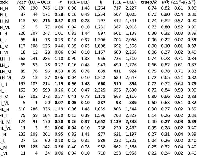
Table S7. Results of estimating the parameters of the Schaefer model with the CMSY method, for 24 simulated stocks. LCL and UCL indicate the lower and upper 95% confidence limits, respectively. Cases where the confidence limits do not include the “true” parameter values are indicated in bold. [SimCatchCPUE_Results_6.xlsx]
Stock MSY (LCL – UCL) r (LCL – UCL) k (LCL – UCL) trueB/k B/k (2.5th-97.5th) HH_H 376 190 745 1.19 0.96 1.48 1,264 717 2,227 0.74 0.82 0.61 0.90 HH_L 87 44 171 0.28 0.16 0.49 1,234 507 3,005 0.73 0.80 0.54 0.89 HH_M 113 59 216 0.57 0.41 0.78 797 412 1,541 0.74 0.82 0.57 0.90 HH_VL 19 5 77 0.06 0.04 0.10 1,231 387 3,918 0.73 0.80 0.52 0.90 HL_H 226 207 247 1.01 0.83 1.44 897 601 1,138 0.30 0.32 0.03 0.39 HL_L 69 61 78 0.23 0.14 0.37 1,206 704 2,068 0.06 0.22 0.02 0.39 HL_M 117 108 126 0.46 0.35 0.65 1,008 692 1,366 0.00 0.10 0.01 0.37 HL_VL 18 12 28 0.06 0.04 0.10 1,167 600 2,268 0.06 0.27 0.02 0.40 HLH_H 262 241 285 1.10 0.90 1.38 956 725 1,210 0.74 0.78 0.71 0.84 HLH_L 65 53 78 0.27 0.16 0.48 943 490 1,776 0.66 0.82 0.61 0.87 HLH_M 85 76 96 0.53 0.39 0.78 639 411 924 0.75 0.78 0.71 0.82 HLH_VL 22 13 37 0.06 0.04 0.10 1,342 680 2,647 0.72 0.65 0.51 0.82 LH_H 197 182 214 1.19 0.96 1.48 660 510 854 0.72 0.72 0.64 0.79 LH_L 152 39 590 0.26 0.16 0.47 2,325 655 7,830 0.72 0.84 0.53 0.90 LH_M 167 102 273 0.57 0.41 0.78 1,178 663 2,116 0.80 0.66 0.52 0.83 LH_VL 5 1 20 0.07 0.05 0.10 287 98 839 0.60 0.63 0.51 0.82 LHL_H 310 286 336 1.19 0.96 1.48 1,039 803 1,344 0.30 0.27 0.02 0.39 LHL_L 79 59 104 0.20 0.13 0.39 1,596 703 2,822 0.14 0.26 0.02 0.39 LHL_M 124 91 170 0.30 0.26 0.37 1,652 1,139 2,238 0.40 0.27 0.08 0.39 LHL_VL 11 3 51 0.06 0.04 0.10 738 220 2,482 0.35 0.28 0.02 0.40 LL_H 233 208 261 0.95 0.82 1.41 977 621 1,197 0.27 0.31 0.04 0.39 LL_L 27 12 60 0.18 0.12 0.32 589 222 1,325 0.04 0.26 0.02 0.40 LL_M 133 125 142 0.56 0.40 0.78 958 662 1,368 0.25 0.32 0.04 0.40 LL_VL 11 4 34 0.06 0.04 0.10 710 258 1,958 0.22 0.24 0.02 0.40
29
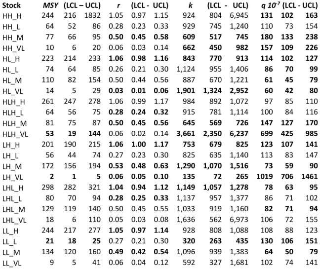
Table S8 shows the BSM estimates of MSY, r, k, and catchability coefficient q compared with the “true”
values used in the simulations. The “true” value of k is 1000 and the “true” value of q is 100*10-7. “True”
MSY is not included in the BSM confidence limits in three of the 24 stocks (13%); “true” r is not included in 12 of the stocks (50%); “true” k is not included in eleven stocks (49%); and “true” q is not included in 16 of the stocks (67%). In comparison, “true” values were missed in only seven stocks with wider confidence limits of the CMSY method and in eight stocks (33%) with the BSM method when biomass instead of CPUE was used. Note that these “miss-rates” are not indicative of the performance of CMSY or BSM against real stocks, because the simulated stocks included some extreme and unlikely scenarios (see catch and biomass patterns in Appendix IV).
Table S8. Results of estimating the parameters of the Schaefer model with the BSM method for CPUE, for 24 simulated stocks, where q is the catchability coefficient. LCL and UCL indicate the lower and upper 95% confidence limits, respectively.
Cases where the confidence limits do not include the “true” parameter value are indicated in bold.
[SimCatchCPUE_Results_6.xlsx]
Stock MSY (LCL – UCL) r (LCL - UCL) k (LCL - UCL) q 10-7 (LCL - UCL) HH_H 244 216 1832 1.05 0.97 1.15 924 804 6,945 131 102 163 HH_L 64 52 86 0.28 0.23 0.33 929 745 1,240 110 73 154 HH_M 77 66 95 0.50 0.45 0.58 609 517 745 180 133 238 HH_VL 10 6 20 0.06 0.03 0.14 662 450 982 157 109 226 HL_H 223 214 233 1.06 0.98 1.16 843 770 913 114 102 127 HL_L 74 64 85 0.26 0.21 0.30 1,124 955 1,406 86 70 99 HL_M 110 82 154 0.50 0.44 0.56 887 670 1,221 61 45 79 HL_VL 14 5 29 0.03 0.01 0.06 1,901 1,324 2,952 60 42 80 HLH_H 261 247 278 1.06 0.99 1.17 984 892 1,072 97 85 110 HLH_L 64 56 75 0.28 0.24 0.32 915 781 1,114 100 84 116 HLH_M 81 75 87 0.50 0.45 0.56 645 569 726 147 127 170 HLH_VL 53 19 144 0.06 0.02 0.14 3,661 2,350 6,237 699 425 985 LH_H 201 190 215 1.06 1.00 1.17 753 679 825 123 107 141 LH_L 56 44 74 0.27 0.23 0.30 825 635 1,140 113 83 147 LH_M 172 156 194 0.53 0.48 0.63 1,290 1,070 1,516 73 59 90 LH_VL 2 1 5 0.06 0.05 0.10 135 72 265 1019 706 1461 LHL_H 298 282 321 1.04 0.94 1.12 1,149 1,057 1,278 78 63 95 LHL_L 80 70 94 0.28 0.25 0.33 1,137 957 1,377 86 71 102 LHL_M 129 119 140 0.50 0.45 0.55 1,033 919 1,160 82 71 94 LHL_VL 18 6 110 0.05 0.03 0.08 1,636 562 6,973 106 72 155 LL_H 244 217 277 1.05 0.97 1.14 928 808 1,088 108 88 123 LL_L 21 18 25 0.27 0.21 0.30 320 263 435 130 106 151 LL_M 134 120 160 0.49 0.42 0.54 1,096 939 1,383 64 50 79 LL_VL 9 5 41 0.06 0.04 0.12 592 327 1,681 102 74 141