prevention of species introductions to freshwater ecosystems
Elizabeta Briski, Stephan Gollasch, Matej David, R. Dallas Linley, Oscar Casas Monroy, Harshana Rajakaruna, and Sarah A. Bailey
Environ. Sci. Technol., Just Accepted Manuscript • DOI: 10.1021/acs.est.5b01795 • Publication Date (Web): 14 Jul 2015 Downloaded from http://pubs.acs.org on July 22, 2015
Just Accepted
“Just Accepted” manuscripts have been peer-reviewed and accepted for publication. They are posted online prior to technical editing, formatting for publication and author proofing. The American Chemical Society provides “Just Accepted” as a free service to the research community to expedite the dissemination of scientific material as soon as possible after acceptance. “Just Accepted” manuscripts appear in full in PDF format accompanied by an HTML abstract. “Just Accepted” manuscripts have been fully peer reviewed, but should not be considered the official version of record. They are accessible to all readers and citable by the Digital Object Identifier (DOI®). “Just Accepted” is an optional service offered to authors. Therefore, the “Just Accepted” Web site may not include all articles that will be published in the journal. After a manuscript is technically edited and formatted, it will be removed from the “Just Accepted” Web site and published as an ASAP article. Note that technical editing may introduce minor changes to the manuscript text and/or graphics which could affect content, and all legal disclaimers and ethical guidelines that apply to the journal pertain. ACS cannot be held responsible for errors or consequences arising from the use of information contained in these “Just Accepted” manuscripts.
Combining ballast water exchange and treatment to maximize prevention of 1
species introductions to freshwater ecosystems 2
3
4
Elizabeta Briski1,2*, Stephan Gollasch3, Matej David4, R. Dallas Linley2, Oscar Casas- 5
Monroy2, Harshana Rajakaruna2 and Sarah A. Bailey2 6
7
8
*Corresponding author: Elizabeta Briski, GEOMAR, Helmholtz-Zentrum für 9
Ozeanforschung Kiel, Düsternbrooker Weg 20, 24105 Kiel, Germany, E-mail:
10
ebriski@geomar.de, elzabriski@yahoo.comm; Phone: +49-431-600-1589; FAX: +49- 11
431-600-4402 12
13
1GEOMAR, Helmholtz-Zentrum für Ozeanforschung Kiel, Düsternbrooker Weg 20, 14
24105 Kiel, Germany 15
2Great Lakes Laboratory for Fisheries and Aquatic Sciences, Fisheries and Oceans 16
Canada, Burlington, Ontario, L7S 1A1, Canada 17
3Gollasch Consulting, Grosse Brunnenstrasse 61, 22763 Hamburg, Germany 18
4Dr. Matej David Consult, Korte 13e, 6310 Izola, Slovenia 19
20
Word count: 6950 21
22
Revised for Environmental Science & Technology (Policy Analysis) 23
ABSTRACT 24
The most effective way to manage species transfers is to prevent their 25
introduction via vector regulation. Soon, international ships will be required to meet 26
numeric ballast discharge standards using ballast water treatment (BWT) systems, and 27
ballast water exchange (BWE), currently required by several countries, will be phased 28
out. However, there are concerns that BWT systems may not function reliably in fresh 29
and/or turbid water. A land-based evaluation of simulated ‘BWE plus BWT’ versus 30
‘BWT alone’ demonstrated potential benefits of combining BWE with BWT for protection 31
of freshwater ecosystems. We conducted ship-based testing to compare the efficacy of 32
‘BWE plus BWT’ versus ‘BWT alone’ on voyages starting with freshwater ballast. We 33
tested the hypotheses that there is an additional effect of ‘BWE plus BWT’ compared to 34
‘BWT alone’ on the reduction of plankton, and that taxa remaining after ‘BWE plus BWT’
35
will be marine (low risk for establishment at freshwater recipient ports). Our study found 36
that BWE has significant additional effect on the reduction of plankton, and this effect 37
increases with initial abundance. As per expectations, ‘BWT alone’ tanks contained 38
higher risk freshwater or euryhaline taxa at discharge, while ‘BWE plus BWT’ tanks 39
contained mostly lower risk marine taxa unlikely to survive in recipient freshwater 40
ecosystems.
41
INTRODUCTION 42
Shipping has been recognized as a primary vector for spread of aquatic species 43
globally.1-5 To prevent arrival of species by ships’ ballast water, Canada, the USA and 44
numerous other countries have implemented regulations requiring transoceanic ships to 45
conduct mid-ocean ballast water exchange (BWE) of tanks that will be discharged into 46
their fresh or marine coastal waters.5-9 In theory, BWE should expel higher risk coastal 47
species into the ocean, replacing them with oceanic species that would have a lower 48
survival probability along the coast. Though observed efficacy of BWE is mixed for 49
marine ecosystems,10-13 the strategy is quite protective of freshwater ecosystems due to 50
osmotic shock.14-17 51
In the near future when the International Convention for the Control and 52
Management of Ships’ Ballast Water and Sediments will enter into force, all commercial 53
ships trading internationally will be required to meet numeric ballast water discharge 54
standards unless granted an exemption based on risk assessment, excepting 55
emergency situations at sea.18-19 It should be noted that this convention does not focus 56
on nonindigenous species, but addresses transfers of all harmful aquatic organisms 57
irrespective of their origin.20 58
Numerous commercial ballast water treatment (BWT) systems that use 59
technologies such as filtration, ultraviolet radiation (UV) or chlorination have been 60
developed5 and BWE will be phased out of use.21-22 The risk of ballast water treated by 61
BWT systems is expected to be lower than that managed by BWE due to lowered 62
propagule pressure; however, there are concerns that BWT systems may not function 63
reliably in fresh and/or turbid water, that the proposed performance standards are not 64
stringent enough, and that BWT systems may fail for mechanical or operational 65
reasons.23-25 Therefore, the government of Canada proposed combining BWE with BWT 66
systems to manage ballast water of ships arriving to freshwater ecosystems in an effort 67
to reap the positive benefits of both management strategies.26 This combined method 68
addresses two factors of the invasion process - reducing propagule pressure through 69
BWT and reducing environmental tolerance through BWE - and is expected to be more 70
effective than either individual method focusing on only a single component. A land- 71
based evaluation of simulated ‘BWE plus BWT’ versus ‘BWT alone’ demonstrated 72
potential benefits of combining BWE with BWT;25 however, a ship-based evaluation was 73
recommended to confirm efficacy and practicality of the combined strategy under real 74
environmental and operational conditions at true size scale.
75
In this study, we conducted ship-based testing to compare the efficacy of ‘BWE 76
plus BWT’ versus ‘BWT alone’ for living organisms ≥ 50 µm in minimum dimension 77
(hereafter zooplankton) and living organisms ≥ 10 and < 50 µm in minimum dimension 78
(hereafter phytoplankton). We tested the hypotheses that: (1) there is an additional 79
effect of BWE on top of ‘BWT alone’ on the reduction of plankton; and (2) taxa present 80
in ballast after ‘BWE plus BWT’ will be low-risk marine species likely unable to survive in 81
freshwater ecosystems.
82
83
METHODS 84
Experimental design 85
Between March 2013 and August 2014, we conducted three trials on three 86
individual ships operating along two routes: two trials between Hamburg (Germany, 87
freshwater) through the Bay of Biscay to the Strait of Gibraltar and one trial between 88
Moerdijk (the Netherlands, freshwater) through the Irminger Basin to Deception Bay 89
(Canada) (Table 1). Each ship had already installed a type-approved BWT system 90
utilizing filtration and electrochlorination, filtration and ultraviolet radiation, or ozonation 91
without filtration (Table 1). The ships were chosen opportunistically as those which 92
already had installed a type-approved BWT system, and which operate on a route 93
permitting uptake of ballast water at a freshwater port followed by BWE, according to 94
the IMO requirements for water depth and distance from the nearest land.18 Each trial 95
consisted of two different experimental treatments: 1) ‘BWT alone’ – tank(s) filled at 96
initial freshwater port and treated with a BWT system; and 2) ‘BWE plus BWT’ – tank(s) 97
filled at initial freshwater port, discharged and refilled in the Atlantic ocean (more than 98
50 nautical miles from the nearest land and in waters of > 200 metres depth), with a 99
BWT system used to treat both the initial port water and the exchanged ocean water.
100
During the first two trials, experimental treatments were run in parallel (two different 101
tanks were used, each for one experimental treatment; Table 1), while operational 102
limitations on the third voyage resulted in the ‘BWT alone’ tank being discharged five 103
days before the ‘BWE plus BWT’ tank (two tanks were used per treatment; the same 104
two tanks were used in time series for both treatments - first for ‘BWT alone’ then for 105
‘BWE plus BWT’ treatment; Table 1). The details on the tanks used, their location on the 106
ships, and capacity are provided in Table 1. Trials lasted between six and 16 days 107
(Table 1).
108
109
Sample collection and enumeration of live/dead organisms 110
Ballast water was sampled each time water was loaded into ballast tanks and 111
during final ballast water discharge. Samples were collected over the whole time that 112
ballast was pumped in (or out) of experimental tanks, resulting in sample volumes 113
between 751 and 1648 L (Table S1). To minimize impacts of organism survival during 114
sample collection and holding time, each sample was collected as two or three 115
sequential subsamples corresponding to the first and second half, or to the beginning, 116
middle, and end of the ballasting process (Table S1).5,27-28 We aimed for three 117
sequential subsamples, however, due to the smaller tank size on the first voyage and 118
corresponding very short ballasting duration, three subsamples were collected only on 119
uptake in Hamburg while two sequential subsamples (i.e., equivalent to the first and 120
second half) were collected during the remainder of the first voyage. All samples were 121
taken from bent elbow pitot tubes installed for scientific sample collection along straight 122
sections of the ballast piping.29 Sampled ballast water was pressure-fed by the ships’
123
ballast system through hoses and PVC tubing equipped with a flow meter into a conical 124
plankton net with 50 µm (in diagonal) mesh within a wetted sample tub. The sample 125
collected inside the plankton net was retained for zooplankton analysis. For 126
phytoplankton, a composite sample totalling to ~ 5 L was taken by collecting ~ 0.5 L of 127
water every one to five minutes during each sampling sequence. Salinity and 128
temperature were measured at two to five minute intervals during the sampling process 129
using a calibrated YSI instrument.
130
Enumeration of live organisms for both taxonomic groups was conducted on 131
board. Zooplankton samples were further concentrated on 50 µm (in diagonal) mesh to 132
100 or 200 mL volume, of which multiple 2 mL subsamples totalling to 6 to 12 mL were 133
analysed, depending on available time and sample complexity. A larger subsample 134
volume could not be processed without exceeding the recommended maximum holding 135
time of 6 hours between completing sample collection and completing sample 136
processing.27-28 The number of fully intact and live individuals of zooplankton in the 137
subsample was determined using a dissecting microscope and standard 138
movement/response to stimuli techniques.30 The counts were recorded according to 139
broad taxonomic groups, such as Copepoda, Cladocera, Rotifera, Bivalvia, Gastropoda, 140
etc. Representative individuals alive in final discharge samples were isolated and 141
preserved separately in > 95% ethanol for later molecular identification.
142
For phytoplankton analysis, one 400 mL subsample was removed from each 143
well-mixed 5 L composite sample, concentrated to 100 mL on 10 µm (in diagonal) mesh 144
and a 5 mL subsample stained using FDA (fluorescein diacetate) as a selective 145
indicator of enzymatic activity. The subsample was processed on board immediately 146
after collection using bright field and epifluorescence microscopy (Zeiss Axiovert A1).31- 147
32 Phytoplankton were not identified to any taxonomic level on board the ship. After 148
staining, the remaining concentrated sample was preserved with Lugol’s iodine solution 149
for later morphological identification. On the first trial, phytoplankton were not 150
enumerated on board during the uptake of ballast in the freshwater port (i.e., Hamburg) 151
due to equipment failure.
152
153
Laboratory enumeration and taxonomic identification 154
After the shipboard trials were completed, preserved samples of zooplankton 155
were examined under a dissecting microscope in entirety; representative individuals of 156
different taxonomic groups were measured and imaged, and twenty individuals from 157
every taxonomic group per sample separated for taxonomic identification. Zooplankton 158
were identified solely by molecular tools in the lab since gross morphological 159
identification was already completed on the ship. DNA was extracted from each whole 160
individual using DNeasy Blood and Tissue Kit (Qiagen Inc., ON, Canada). Fragments of 161
the mitochondrial genes COI and 16S were amplified using the universal COI primers 162
LCO1490 and HCO2190,33 and 16S primers S1 and S2.34 PCR reactions followed the 163
protocol from previous studies,35 and PCR products were sequenced using an ABI 164
3130XL automated sequencer (Applied Biosystems, Foster City, CA). Recovered DNA 165
sequences were blasted against those in the GenBank database 166
(http://blast.ncbi.nlm.nih.gov/Blast.cgi) using the nucleotide blast. The scores resulting 167
in at least 98% similarity to the closest match for COI and 99% for 16S were deemed 168
species level identifications. Freshwater, brackish and/or marine natural habitats of 169
identified species were assigned based on scientific literature review.
170
Preserved samples of phytoplankton were mixed by overturning by hand more 171
than 20 times, and a volume of 50 mL per sample put in a settling column for 24 172
hours.36 Phytoplankton were enumerated and identified morphologically using a Nikon 173
AZ100 inverted microscope. There was no molecular identification of phytoplankton.
174
Identifications were based on literature references.37-41 Only intact cells with clearly 175
visible cell content were assessed. Freshwater, brackish and/or marine natural habitats 176
of identified species were assigned based on review of scientific literature and 177
taxonomic websites.
178
179
Statistical analysis 180
We tested whether there is an additional effect of ‘BWE plus BWT’ on the 181
reduction of plankton abundance compared to that of ‘BWT alone’. To test this 182
hypothesis, we used abundance estimates of both zooplankton and phytoplankton 183
samples collected after treatments (i.e., ‘BWE plus BWT’ and ‘BWT alone’) at three 184
sequential time-segments from each of three ship trials (subjects). This allowed 185
samples collected during the same time-segments within each ship to be statistically 186
paired. We computed the proportions (i.e., abundances in ‘BWT alone’/abundances in 187
‘BWE plus BWT’) for each pair of samples within each ship trial as the dependent 188
variable, and used the log10 transformation to meet the assumption of normality, which 189
we denote by y hereafter. We used the (log10) abundance of ‘BWT alone’ samples as 190
the independent variable, which we denote by T hereafter. To test the above 191
hypothesis, we tested if y (i.e., difference in log densities between ‘BWT alone’ and 192
‘BWE plus BWT’) increases with increasing T (i.e., densities after 'BWT alone'), such 193
that y > 0 (i.e., the difference is positive), using linear mixed effect models, incorporating 194
random effects due to ships (Ships), and fixed effects due to sequential time-segments 195
(Time) and plankton type (ZorP) nested within fixed effects of T. The resulting three 196
alternative models that we analysed using the Linear Mixed Effect Model procedure in 197
SPSS version 2242 are given in Table 2 with detailed descriptions.
198
Note that, as we selected three ships from a larger population of ships, here, we 199
would more naturally treat the variable "Ship" as a random effect. That is, we would 200
regard the effects of ship as a random sample of the effects of all the ships in the full 201
population of ships. We would treat explanatory variables T, T(ZorP), and T(Time) as 202
fixed effects, assuming there is no randomness in their choice, rather that they are fixed 203
or specific, or the average responses for all subjects. Our choice of linear mixed effect 204
models is because they allow incorporating both fixed and random effects into linear 205
models (a regression type with a hierarchical structure), such that, random effects can 206
account for individual differences in response to an effect, while fixed effect estimate the 207
population level coefficients. Although, we tested numerous other models with different 208
structures and combinations of variables, incorporating non-linear effects also, here, we 209
present only these three alternative nested models as other ones did not improve the 210
goodness of fitness drastically, compared to these three, based on Akaike Information 211
Criteria (AIC).
212
In these models (Table 2), the response variable y was unitless, and the 213
predictor variable T was in two different scales, m-3 and mL-1, corresponding to factors Z 214
(zooplankton) and P (phytoplankton), respectively. This scaling was used because the 215
management regulations of the two types of organisms are implemented in these two 216
scales.18 Therefore, the models quantify scale-free effects on the response variable as a 217
function of the predictor variable, given in two different management scales, 218
corresponding to plankton type. In all these models, we incorporated Time-segment as 219
a repeated measure (RM) (or a repeated effect), with repeated covariance type - scaled 220
identity, and random effects covariance type - variance components. Using each model 221
with and without incorporation of random effects yielded a total of six alternative models.
222
We used the maximum likelihood estimator in the Mixed Effect Model methodology in 223
SPSS for model parameterization, and AIC for model comparison.
224
Additionally, we tested the significance of the difference in abundances of 225
plankton type (zooplankton and phytoplankton) between freshwater ports and the ocean 226
to see if treatment of ocean water would require less effort than treatment of fresh water 227
by BWT systems. To test this hypothesis, we transformed the abundance data by log10
228
to meet the normality assumption, and used paired differences between the ocean and 229
freshwater port samples. For this, we used the Markov Chain Monte Carlo (MCMC) 230
simulation procedure in Poptools (Ver. 3.2): First, we randomly resampled freshwater 231
port abundance data (i.e., the 3 repeated samples) within each ship, and randomly 232
paired them with the ocean abundance data (i.e., the 3 repeated samples) of the same 233
ship, and calculated the average difference in log10 abundances between freshwater 234
ports and ocean intakes across all ships. We repeated this resampling scheme 100 235
times yielding 100 test values (i.e., the average differences). Then, from each simulated 236
100 resamples above, we generated another 1000 resamples by randomly mixing both 237
the ocean and freshwater port abundance data (of the 3 repeated samples) within each 238
ship. This yielded the theoretical distribution (i.e., the dependent values) of the average 239
differences of log10 abundances for the case where there is no systematic difference in 240
abundances due to ocean and freshwater port intakes, which is the case if the null 241
hypothesis were true. The p-value for the hypothesis, that "there is a difference in 242
abundance of taxa between freshwater port and the ocean intakes", is given by the 243
proportion of simulated resamples (i.e., 105) that yielded dependent values greater than 244
the test values. We did this hypothesis test for phytoplankton and zooplankton 245
separately, and also for both taken together.
246
247
RESULTS 248
Community composition of initial freshwater ballast water 249
Live zooplankton and phytoplankton abundances determined on board in 250
samples collected during ballast uptake in Hamburg/Moerdijk ranged from 1198 to 251
49,907 individuals per m3 and from 261 to 1145 cells per mL, respectively (Table S1).
252
Copepoda and Rotifera were dominant zooplankton taxa at source ports ranging 253
between 30% and 76%, and 16% and 68% abundance, respectively (Table S2). Across 254
all trials, laboratory identification of preserved samples revealed at least two Bivalvia, 255
six Cladocera, twelve Copepoda, one Nematoda, six Rotifera, and one Trematoda 256
species (Table S3). All zooplankton species are considered freshwater or euryhaline 257
species, except one Copepoda (Clausocalanus pergens) which is previously reported 258
only as a marine species (Table S3). Since species-level identifications for uptake 259
samples were conducted on composite preserved samples, we cannot be certain that 260
the specimen was alive at the time of collection. Laboratory identification of preserved 261
phytoplankton taxa indicated that Bacillariophyceae and Dinophyceae were dominant 262
taxa ranging from 14% to 92%, and 4% and 82% abundance, respectively (Table S4).
263
Chlorophyceae ranged from 1% to 25% (Table S4). Across all trials, at least five 264
Chlorophyceae, two Chrysophyceae, seven Dinophyceae, 33 Bacillariophyceae, one 265
Cyanophyceae, and one Dictyochophyceaespecies were identified (Table S5). Salinity 266
of water pumped into the tanks ranged from 0.3 – 0.5 ppt (Table S1), but interestingly at 267
least two Dinophyceae, eleven Bacillariophyceae, and one Dictyochophyceaespecies 268
are to our knowledge marine species, unable to survive in freshwater habitats (Table 269
S5). Again, we cannot be certain that the individuals of these species were alive at the 270
time of collection (see discussion).
271
272
Community composition of exchanged oceanic ballast water 273
Live zooplankton and phytoplankton abundances determined on board in 274
samples collected during BWE in the Bay of Biscay/Irminger Basin ranged from 791 to 275
4527 individuals per m3 and from 10 to 2983 cells per mL, respectively (Table S1).
276
Nearly all live zooplankton taxa observed on board the ships were Copepoda (99%;
277
Table S2). Laboratory identification of preserved samples revealed at least 15 278
Copepoda, two Decapoda, one Gastropoda, and two Thecostraca species across trials 279
- all are considered marine or euryhaline species (Table S3). Laboratory identification of 280
preserved phytoplankton indicated that Bacillariophyceae were dominant taxa in all 281
trials ranging from 93% to 100% (Table S4). In all trials together, at least three 282
Chlorophyceae, six Dinophyceae, 24 Bacillariophyceae, three Ciliophora, one 283
Dictyochophyceae, and two additional species were identified – all are considered 284
marine or euryhaline taxa (Table S5). Salinity of water pumped into the tanks during 285
BWE ranged from 33.5 – 35.3 ppt (Table S1). Statistical comparison of abundance of 286
taxa between freshwater ports and the ocean determined significantly lower abundance 287
of taxa in the ocean: p = 0.001 for pooled data, p = 0.006 for zooplankton and p = 0.02 288
for phytoplankton.
289
290
Community composition at final ballast water discharge 291
Live zooplankton abundances in samples collected during discharge of ‘BWT 292
alone’ tanks ranged from 0 to 11,092 individuals per m3; those of live phytoplankton 293
ranged from 2 to 174 cells per mL (Table S1). Copepoda represented 99% of live taxa 294
observed on board the ships (Table S2). Laboratory identification revealed at least one 295
Amphipoda, four Cladocera, six Copepoda, and one Nematoda species across trials, all 296
of which are expected to thrive in freshwater habitats (Table S3). Laboratory 297
identification of preserved phytoplankton taxa indicated that Bacillariophyceae 298
dominated the first and third trials (98% and 100%, respectively), while Chlorophyceae 299
were most abundant in the second trial (88%; Table S4). Most species observed are 300
previously reported from freshwater habitats, however, in addition to the seven ‘marine’
301
species observed during initial uptake, at least five new ‘marine’ species were detected 302
that to our knowledge are unable to survive in freshwater habitats (four Dinophyceae 303
and one Ciliophora species; Table S5). Again, since species identification was 304
conducted on preserved samples, there might be alternative explanations for the 305
observations.
306
In the case of ‘BWE plus BWT’ tanks, live zooplankton abundances in samples 307
collected during discharge ranged from 0 to 124 individuals per m3; those of live 308
phytoplankton ranged from 0 to 1662 cells per mL (Table S1). Copepoda represented 309
100% of live taxa in the first two trials, while in the third trial 86% were other taxa (Table 310
S2). Laboratory identification revealed at least two Bivalvia, four Cladocera, ten 311
Copepoda, one Gastropoda, one Nematoda, and one Rotifera species (Table S3). All 312
zooplankton observed alive at the time of sampling are considered marine or euryhaline 313
(Table S3). Laboratory identification of preserved phytoplankton showed that 314
Bacillariophyceae were dominant in all trials ranging from 57% to 88% abundance, 315
followed by Chlorophyceae ranging from 11% to 23% abundance (Table S4). All 316
phytoplankton identified are considered marine or euryhaline species (Table S5).
317
Salinity of ballast water discharged ranged from 0.3 – 3.8 ppt and 29.7 – 32.9 ppt for 318
‘BWT alone’ and ‘BWE plus BWT’ tanks, respectively (Table S1).
319
320
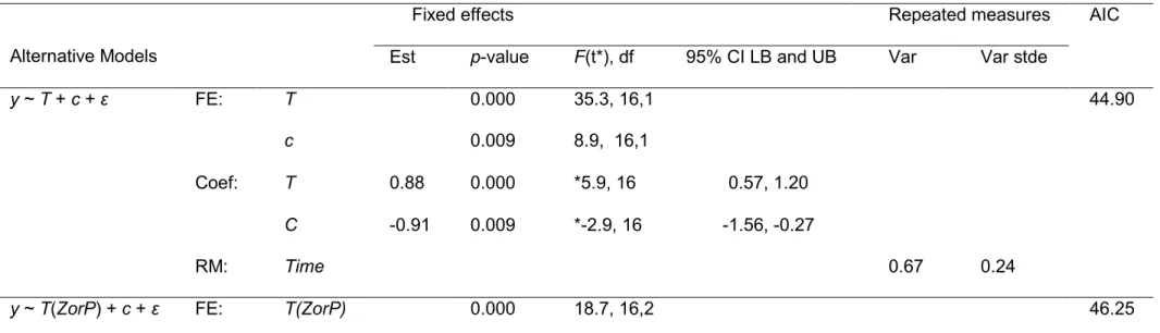
Efficacy of ‘BWT alone’ versus ‘BWE plus BWT’
321
All three fixed effect models (Table 3) yielded significant relationships (gradient >
322
0) between log10 (abundances in ‘BWT alone’/abundances in ‘BWE plus BWT’) and 323
log10 (‘BWT alone’) with p < 0.001. The predictive log10 (‘BWT alone’), nested with 324
plankton type (ZorP), yielded a significantly positive gradient of 1.06 for factor Z, and 325
0.87 for factor P (p < 0.001). The incorporation of nested effects to model gradient was 326
also significant (p < 0.001, F = 18.7, df = 16,2). Similarly, predictive log10 (‘BWT alone’), 327
nested with factor Time, yielded significantly positive gradients 0.94, 0.95, and 0.74 (p <
328
0.01), and the incorporation of nested effects to model-gradient was also significant (p <
329
0.001, F = 12.8, df = 16,3). Random effects due to type of plankton (ZorP) and Time 330
were redundant, as they did not improve their respective fixed effect models, so that 331
they are not presented here (Table 3). The AIC values suggested that the simplest 332
model, given by y ~ T + c + ɛ, was the best predictive model (p < 0.001, F = 35.3, df = 333
16,1), demonstrating that regardless of the plankton type or sequential subsample time 334
factor, BWE has an additional effect on the reduction of plankton abundance with R2 = 335
0.69 (Table 3). The effect of reduction in abundance increases with increasing plankton 336
abundance in ‘BWT alone’ tanks; a positive effect was not apparent at very low 337
abundances (Fig. 1).
338
339
DISCUSSION 340
Our study found that BWE used in combination with BWT provides a significant 341
additional reduction of plankton abundance, and this effect increases with greater 342
abundance (after treatment) in ‘BWT alone’ tanks. As per expectations, ‘BWT alone’
343
tanks filled in freshwater ports contained mainly freshwater or euryhaline taxa at 344
discharge, while ‘BWE plus BWT’ tanks contained mainly marine taxa that primarily 345
originated from the BWE area, and would likely not survive if discharged into freshwater 346
ecosystems. Due to the almost exclusively marine composition of live zooplankton taxa 347
after BWE, the ‘BWE plus BWT’ strategy notably reduces introduction risk of 348
zooplankton through environmental mismatching. The environmental mismatching effect 349
is less clear for phytoplankton, since many marine and euryhaline species were 350
observed in the initial ballast water uptake sample of the freshwater ports though it is 351
unknown if they were alive. Notably, there were no freshwater phytoplankton species 352
observed in discharge samples of the ‘BWE plus BWT’ experiments. A recent study 353
examining BWE plus chlorination versus BWE or chlorination alone found similar 354
results, with the hybrid treatment generally having lowest densities of plankton and 355
microbes at discharge, although they did not assess the risk of the species composition 356
resulting from the different management strategies.43 357
When BWE was first introduced, it was presumed that incoming ocean taxa 358
would be both lower in density and have a lower survival probability along the coast 359
than those taken up at coastal ports.44 Empirical studies conducted since then have 360
indicated that both abundance and species richness of plankton may increase 361
immediately after BWE,10,45-46 but that longer voyages result in lower abundance and 362
species richness of zooplankton and diatoms, and lower species richness of 363
dinoflagellates due to mortality.2,46-49 During our trials, plankton abundance was 364
consistently lower in the ocean than in coastal freshwater ports. As a result, BWE used 365
in combination with BWT might result in additional benefit by lowering the ‘challenge’
366
faced by the BWT systems.
367
While we are expecting that BWT systems will greatly reduce transport and 368
introduction of aquatic species into new habitats, our study demonstrates that taxa such 369
as Copepoda, Gastropoda and Nematoda may survive BWT applications. In particular, 370
Copepoda were recorded alive after all three trials. As transport vectors change through 371
time, the associated species assemblage will also change, such as when the 372
replacement of solid ballast with ballast water in the late nineteenth century led to a 373
change in ship-mediated introductions from insects, plants, and earthworms to aquatic 374
taxa.5,50 Previous studies testing BWT systems similarly observed that smaller, soft- 375
body zooplankton and/or zooplankton with small juvenile stages such as Rotifera, 376
Copepoda, or Mollusca selectively survived treatment.32,51 With the application of BWT 377
systems in the future, under both ‘BWT alone’ and ‘BWE plus BWT’ scenarios, we may 378
observe a reduction in the rate of establishment of new species, with selection towards 379
Copepoda as forthcoming aquatic non-indigenous taxa. Similar taxonomic shifts may be 380
expected in phytoplankton as well.
381
The zooplankton taxonomic composition in the two freshwater ports used as 382
starting points for our trials was composed of freshwater or euryhaline species, with only 383
one marine species recorded; interestingly, beside freshwater or euryhaline species of 384
phytoplankton identified, at least 14 phytoplankton species found in the ballast water at 385
uptake are considered marine. Our phytoplankton species identifications were 386
completed several months after the trials on Lugol’s solution preserved samples, 387
therefore, it is not clear if the marine species recovered were alive during the trials.
388
Possibly, these species were present as contaminants in the ballast pipework of the 389
ships, or might have been recently discharged into the ports by other ships but due to 390
mismatch in environmental conditions were in a state of dying or already dead.
391
Furthermore, the port of Hamburg is located in an inner estuary with tidal amplitude of 392
more than 2 m, thus marine species could possibly occur as a result of tidal water influx.
393
The long term viability of those individuals in freshwater would again be questionable.
394
On the other hand, a more intriguing explanation might be that some, or even all of 395
those species, were alive and established in the freshwater port ecosystems. Some 396
marine species discovered in our study have already been reported in the estuarine 397
Elbe River and the freshwater Port of Hamburg.52 Invasions of freshwater habitats by 398
marine and brackish species have become increasingly common in recent years.53-54 399
Most biodiversity studies are conducted in protected areas and habitats less impacted 400
by human activities, so consequently, our knowledge on biodiversity in ports - invasion 401
hubs - is often poor.
402
This study is the first research conducted on operational ships fitted with type 403
approved BWT systems to test BWT in combination with BWE as a ballast water 404
management method, as well as its efficacy compared with BWT systems alone. While 405
our purpose was not to confirm compliance with any ballast water discharge standard, 406
we observed that efficacy among the three different BWT systems was quite mixed.
407
There are several sources of error which can affect the accuracy of numeric organism 408
counts obtained during our testing, including sample collection method, sample size, 409
and conditions encountered on board ships (e.g., vibration, ship rolling and pitching). As 410
a result, our counts should be viewed as an ‘estimate’ of plankton density, perhaps 411
accurate only within one order of magnitude. With this in mind, it appears that the BWT 412
systems more effectively managed zooplankton on the first two voyages than on the 413
third voyage. Conversely, BWT appeared least effective for phytoplankton on the 414
second voyage. In general, our past experience indicates that most BWT systems utilize 415
a two-stage process to separately manage zooplankton (e.g., filtration) and 416
phytoplankton (e.g., chlorination or UV). As the BWT system on the third voyage utilized 417
only a single stage treatment process (i.e., ozone), the variability in zooplankton 418
densities at discharge across voyages might be attributed to the absence of a filter. The 419
higher density of phytoplankton observed on the second voyage is possibly explained 420
by the delayed metabolic reaction to ultraviolet radiation as measured by FDA 421
staining.55 The efficacy of BWT systems might also be affected by environmental factors 422
such as temperature, turbidity, or ionic composition (salinity) of the water; due to the 423
small sample size in our study, we were not able to test for the effect of environmental 424
factors.
425
The invasion process consists of a series of stages, with successful transition 426
between stages dependent on the abundance of individuals introduced, their tolerance 427
to environmental conditions in a new habitat, and assimilation into the biological 428
community.5,56-57 As a result, the combined ‘BWE plus BWT’ strategy that targets two 429
factors in the invasion process (i.e., propagule pressure and environmental tolerance) 430
proved to be more effective in reducing invasion risk to freshwater recipient systems 431
than ‘BWT alone’. However, we noted exceptions to the effect of environmental 432
mismatch during our study, and caution that marine species released into freshwater 433
habitats could potentially adapt to lower salinity.53-54 Consequently, more studies 434
exploring rapid evolution, species adaptation and phenotypic plasticity during the 435
invasion process would be informative.58 Furthermore, additional tests to determine 436
precision and accuracy of different ballast water sampling and analysis protocols are 437
needed to quantify sampling and counting error, in order to improve assessments of 438
plankton density in treated ballast water discharges.27-28 439
440
ACKNOWLEDGEMENT 441
We thank all ship crews, agents, operators, and owners, manufacturers of the 442
BWT systems, and the mine Canadian Royalties Inc. for their participation and support 443
of this research. We appreciate the assistance of Julie Vanden Byllaardt and Sara 444
Ghabooli with sample collection and molecular taxonomy, respectively. We also thank 445
the three anonymous referees for constructive comments. This research was supported 446
by Transport Canada and Fisheries and Oceans Canada, both directly and through the 447
NSERC Canadian Aquatic Invasive Species Network, and by an NSERC Discovery 448
Grant awarded to SAB. EB was supported by the Alexander von Humboldt Sofja 449
Kovalevskaja Award.
450
451
Supporting Information Available 452
The Supporting Information is available free of charge via the Internet at 453
http://pubs.acs.org.
454
455
REFERENCES 456
(1) Ricciardi, A. Patterns of invasion in the Laurentian Great Lakes in relation to 457
changes in vector activity. Divers. Distrib. 2006, 12, 425-433.
458
(2) David, M.; Gollasch, S.; Cabrini, M.; Perkovič, M. Bošnjak, D.; Virgilio, D. Results 459
from the first ballast water sampling study in the Mediterranean Sea – the Port of 460
Koper study. Mar. Pollut. Bull. 2007, 54, 53-65.
461
(3) Molnar, J. L.; Gamboa, L. R.; Revenga, C.; Spalding, M. D. Assessing the global 462
threat of invasive species to marine biodiversity. Front. Ecol. Environ. 2008, 6, 485- 463
492.
464
(4) Hulme, P. E. Trade, transport and trouble: managing invasive species pathways 465
in an era of globalization. J. Appl. Ecol. 2009, 46, 10-18.
466
(5) David, M.; Gollasch, S. Global Maritime Transport and Ballast Water 467
Management – Issues and Solutions; Invading Nature. Springer Series in Invasion 468
Ecology 8, Springer Science + Business Media, Dordrecht, The Netherlands, 2015.
469
(6) United States Coast Guard. Ballast Water Management for Control of Non- 470
indigenous Species in Waters of the United States. Code of Federal Regulations, 33- 471
CFR Part 151, Subpart D; 1998; Available from 472
http://www.gpo.gov/fdsys/search/home.action United States Environmental 473
Protection Agency. Generic Protocol for the Verification of Ballast Water Treatment 474
Technology. EPA/600/R-10/146; 2010; Available from 475
http://www.epa.gov/nscep/index.html 476
(7) Government of Canada. Ballast Water Control and Management Regulations.
477
Canada Gazette; 2006, 140(13); Available from 478
http://gazette.gc.ca/archives/p2/2006/2006-06-28/html/sor-dors129-eng.html 479
(8) New Zealand Government. Requirements for Vessels Arriving in New Zealand.
480
Ministry for Primary Industries. 2010; Available at:
481
http://www.biosecurity.govt.nz/enter/ships 482
(9) Australian Government. Australian Ballast Water Management Requirements - 483
Version 5. 2011; Available at:
484
http://www.daff.gov.au/biosecurity/avm/vessels/quarantine- 485
concerns/ballast/australian-ballast-water-management-requirements 486
(10) McCollin, T.; Shanks, A. M.; Dunn, J. The efficiency of regional ballast water 487
exchange: Changes in phytoplankton abundance and diversity. Harmful Algae 2007, 488
6, 531-546.
489
(11) Ruiz, G.M.; Reid, D.F. Current state of understanding about the effectiveness 490
of ballast water exchange (BWE) in reducing aquatic nonindigenous species (ANS) 491
introductions to the Great Lakes basin and Chesapeake Bay, USA: Synthesis and 492
analysis of existing information. NOAA Technical Memorandum GLERL-142; 2007;
493
Available at: ftp://ftp.glerl.noaa.gov/publications/tech_reports/glerl-142/tm-142.pdf 494
(12) Briski, E.; Bailey, S. A.; MacIsaac, H. J. Invertebrates and their dormant eggs 495
transported in ballast sediments of ships arriving to the Canadian coasts and the 496
Laurentian Great Lakes. Limnol. Oceanogr. 2011, 56, 1929-1939.
497
(13) Briski, E.; Bailey, S.A.; Casas-Monroy, O.; DiBacco, C.; Kaczmarska, I.;
498
Lawrence, J.E.; Leichsenring, J.; Levings, C.; MacGillivary, M.L.; McKindsey, C.W.;
499
Nasmith, L.E.; Parenteau, M.; Piercey, G.E.; Rivkin, R.B.; Rochon, A.; Roy, S.;
500
Simard, N.; Sun, B.; Way, C.; Weise, A.M.; MacIsaac, H.J. Taxon- and vector- 501
specific variation in species richness and abundance during the transport stage of 502
biological invasions. Limnol. Oceanogr. 2013, 58, 1361-1372.
503
(14) Gray, G. K.; Johengen, T. H.; Reid, D. F.; MacIsaac, H. J. Efficacy of open- 504
ocean ballast water exchange as a means of preventing invertebrate invasions 505
between freshwater ports. Limnol. Oceanogr. 2007, 5, 2386-2397.
506
(15) Briski, E.; Bailey, S. A.; Cristescu, M. E.; MacIsaac, H. J. Efficacy of ‘saltwater 507
flushing’ in protecting the Great Lakes from biological invasions by invertebrate eggs 508
in ships’ ballast sediment. Freshwater Biol. 2010, 55, 2414-2424.
509
(16) Bailey, S. A.; Deneau, M. G.; Jean, L.; Wiley, C. J.; Leung, B.; MacIsaac, H. J.
510
Evaluating efficacy of an environmental policy to prevent biological invasions.
511
Environ. Sci. Technol. 2011, 45, 2554-2561.
512
(17) Reid, D. F. The role of osmotic stress (salinity shock) in protecting the Great 513
Lakes from ballast-associated aquatic invasions. Technical Report. U.S. Saint 514
Lawrence Seaway Development Corporation. U.S. Department of Transportation.
515
2012; Available from http://www.greatlakes- 516
seaway.com/en/pdf/BWE_Osmotic_Shock_Report_11_30_12.pdf 517
(18) International Maritime Organization. International Convention for the Control 518
and Management of Ships Ballast Water and Sediments. As adopted by consensus 519
at a Diplomatic Conference at IMO, London, England; 2004; Available from 520
www.imo.org/About/Conventions/ListOfConventions/Pages/International-Convention- 521
for-the-Control-and-Management-of-Ships%27-Ballast-Water-and-Sediments- 522
(BWM).aspx 523
(19) International Maritime Organization. Application of the international convention 524
for the control and management of ships' ballast water and sediments, 2004.
525
Assembly 28th session, 28 January 2014. A 28/Res.1088. International Maritime 526
Organization, London, England; 2014; Available from:
527
http://www.mardep.gov.hk/en/msnote/pdf/msin1408anx1.pdf 528
(20) David, M.; Gollasch, S.; Leppäkoski, E. Risk assessment for exemptions from 529
ballast water management – The Baltic Sea case study. Mar. Pollut. Bull. 2013, 75, 530
205-217.
531
(21) Gollasch, S.; David, M.; Voigt, M.; Dragsund, E.; Hewitt, C. L.; Fukuyo, Y.
532
Critical review of the IMO international convention on the management of ships’
533
ballast water and sediments. Harmful Algae, 2007, 6, 585-600.
534
(22) David, M.; Gollasch, S. EU shipping in the dawn of managing the ballast water 535
issue. Mar. Pollut. Bull. 2008, 56(12), 1966-1972.
536
(23) United States Environmental Protection Agency. Generic Protocol for the 537
Verification of Ballast Water Treatment Technology. EPA/600/R-10/146; 2010;
538
Available from http://www.epa.gov/nscep/index.html 539
(24) National Research Council. Assessing the Relationship between Propagule 540
Pressure and Invasion Risk in Ballast Water; The National Academic Press, 541
Washington, D.C., 2011.
542
(25) Briski, E.; Allinger, L.E.; Balcer, M.; Cangelosi, A.; Fanberg, L.; Markee, T.P.;
543
Mays, N.; Polkinghorne, C.N.; Prihoda, K.R.; Reavie, E.D.; Regan, D.H.; Reid, D.M.;
544
Saillard, H.J.; Schwerdt, T.; Schaefer, H.; TenEyck, M.; Wiley, C.J.; Bailey, S.A.
545
Multidimensional approach to invasive species prevention. Environ. Sci. Technol.
546
2013, 47, 1216-1221.
547
(26) International Maritime Organization. Development of Guidelines and Other 548
Documents for Uniform Implementation of the 2004 BWM Convention. Proposal to 549
Utilize Ballast Water Exchange in Combination with a Ballast Water Management 550
System to Achieve an Enhanced Level of Protection. Submitted by Canada.
551
International Maritime Organization, Sub-Committee on Bulk Liquids and Gases, 552
London, England; 2010; Available from:http://www.uscg.mil/imo/blg/docs/blg16- 553
report.pdf 554
(27) Gollasch, S.; David, M. Testing sample representativeness of a ballast water 555
discharge and developing methods for indicative analysis. European Maritime Safety 556
Agency (EMSA), Lisbon, Portugal, 2010; Available from 557
http://www.emsa.europa.eu/psc-main/thetis/151-ballast-water/605-report-testing- 558
sample-representativeness-of-a-ballast-water-discharge-and-developing-methods- 559
for-indicative-analysis.html 560
(28) Gollasch, S.; David, M. Recommendations for Representative Ballast Water 561
Sampling. Final report of research study of the Bundesamt für Seeschifffahrt und 562
Hydrographie, Hamburg, Germany. Order Number 4500025702, 2013.
563
(29) Richard, R. V.; Grant, J. F.; Lemieux, E. J. Analysis of ballast water sampling 564
port designs using computational fluid dynamics. Report No. CG-D-01-08 Groton:
565
U.S. Coast Guard Research and Development Center. 2008; Available at:
566
http://www.uscg.mil/hq/cg9/rdc/Reports/2008/2008-0180a.pdf 567
(30) International Maritime Organization. Guidance on ballast water sampling and 568
analysis for trial use in accordance with the BWM Convention and Guidelines (G2).
569
International Maritime Organization, London, England; 2013; Available from:
570
http://globallast.imo.org/wp-content/uploads/2015/01/BWM.2-Circ.42.pdf 571
(31) Adams, J. K.; Briski, E.; Ram, J. L.; Bailey, S. A. Evaluating the response of 572
freshwater organisms to vital staining. Manage. Biol. Invasions 2014, 5(3), 197-208.
573
(32) Briski, E.; Linley, R.D.; Adams, J.; Bailey, S.A. Evaluating efficacy of a ballast 574
water filtration system for reducing spread of aquatic species in the Great Lakes.
575
Manage. Biol. Invasions 2014, 5(3), 245-253.
576
(33) Folmer, O.; Black, M.; Hoeh, W.; Lutz, R.; Vrijenhoek, R. DNA primers for 577
amplification of mitochondrial cytochrome c oxidase subunit I from diverse metazoan 578
invertebrates. Mol Mar Biol and Biotechnol, 1994, 3, 294-299.
579
(34) Palumbi, S. Nucleic acids II: The polymerase chain reaction. In Molecular 580
Systematics; Hillis, D., Mable, B., Moritz, C., Eds.; Sinauer: Sunderland MA 1996 pp 581
205-247.
582
(35) Briski, E.; Cristescu, M.E.; Bailey, S.A.; MacIsaac, H.J. Use of DNA barcoding 583
to detect invertebrate invasive species from diapausing eggs. Biol. Invasions 2011, 584
13, 1325-1340.
585
(36) Utermöhl H. Zur Ver Vervollkommnung der quantitativen Phytoplankton- 586
Methodik. Mitt. inc. Ver. theor. angew. Limnol. 1958, 9, 1-38.
587
(37) Bérard-Therriault, L.; Poulin, M.; Bossé, L. Guide d’Identification du 588
Phytoplancton Marin de l’Estuaire et du Golfe du Saint-Laurent; Publication Spéciale 589
Canadienne des Sciences Halieutiques et Aquatiques 128, 1999.
590
(38) Taylor, F. J. R.; Fukuyo, Y.; Larsen, J.; Hallegraeff, G. M. Taxonomy of harmful 591
dinoflagellates. In Manual on Harmful Marine Microalgae. Monographs on 592
Oceanographic Methodology 11; Hallegraeff, G. M., Anderson, D. M., Cembella, A.
593
D., Eds.; UNESCO Publishing: France, pp 389-432; 2003.
594
(39) Throndsen, J.; Hasle, G.; Tangen, K. Phytoplankton of Norwegian Coastal 595
Waters; Almater Forlag AS, Oslo. 2007.
596
(40) Huynh, M.; Serediak, N. Algae Identification Field Guide. Agriculture and Agri- 597
Food Canada. 2011.
598
(41) Bellinger, E. G; Sigee, D. C. Freshwater Algae. Identification and Use as 599
Bioindicators; John Wiley & Sons, Ltd., 2010.
600
(42) SYSTAT Software. Linear mixed-effects modeling in SPSS – An introduction to 601
the mixed procedure. Technical Report. 2004; Available at:
602
http://www.spss.ch/upload/1107355943_LinearMixedEffectsModelling.pdf 603
(43) Paolucci, E.M.; Hernandez, M.R.; Potapov, A.; Lewis, M.A.; MacIsaac, H.J.
604
Hybrid system increases efficiency of ballast water treatment. J. Appl. Ecol. 2015, 52, 605
348-357.
606
(44) Bailey, S.A. An overview of thirty years of research on ballast water as a vector 607
for aquatic invasive species to freshwater and marine environments. Aquat. Ecosyst.
608
Health Manag. 2015, 18, doi: 10.1080/14634988.2015.1027129.
609
(45) Simard, N.; Plourde, S.; Gilbert, M.; Gollasch, S. Net efficacy of open ocean 610
ballast water exchange on plankton communities. J. Plankton Res. 2011, 33, 1378- 611
1395.
612
(46) Chan, F. T.; Bradie, J.; Briski, E.; Bailey, S. A.; Simard, N.; MacIsaac, H. J.
613
Assessing introduction risk using species' rank-abundance distributions. P. Roy. Soc.
614
B – Biol. Sci. 2015, 282, doi: 10.1098/rspb.2014.1517.
615
(47) Gollasch, S.; Lenz, J.; Dammer,; M.; Andres, H. G. Survival of tropical ballast 616
water organisms during a cruise from the Indian Ocean to the North Sea. J. Plankton.
617
Res. 2000, 22, 923-937.
618
(48) Olenin, S.; Gollasch, S.; Jonushas, S.; Rimkute, I. 2000 En-route investigations 619
of plankton in ballast water on a ships’ voyage from the Baltic Sea to the open 620
Atlantic coast of Europe. Int. Rev. Hydrobiol. 2000, 85, 577-596.
621
(49) Briski, E.; Chan, F.; MacIsaac, H. J.; Bailey, S. A. A conceptual model of 622
community dynamics during the transport stage of the invasion process: a case study 623
of ships' ballast. Divers. Distrib. 2014, 20, 236-244.
624
(50) Lockwood, J. L.; Hoopes, M. F.; Marchetti, M. P. Invasion Ecology; Blackwell 625
Publishing, Oxford, 2007.
626
(51) Cangelosi, A.A.; Mays, N.L.;Balcer, M.D.; Reavie, E.D.; Reid, D.M.; Sturtevant 627
,R.; Gao, X. The response of zooplankton and phytoplankton from the North 628
American Great Lakes to filtration. Harmful Algae, 2007, 6, 547–566.
629
(52) Herr, W.; Gerdes, J.-U.; Kroker, J.; Herr, T. M.; Ritcher, R.; Schammey, A.
630
Anpassung der Fahrrinne von Unter- und Außenelbe an die Containerschifffahrt.
631
Planfeststellungsunterlage nach Bundeswasserstraßengesetz. Schutzgut Tiere und 632
Pflanzen, aquatisch- Teilgutachten Aquatische Flora -(Bestand und Prognose).
633
Unterlage H.5a; Wasser- und Schifffahrtsverwaltung des Bundes, Wasser- und 634
Schifffahrtsamt Hamburg und Freie und Hansestadt Hamburg, Hamburg Port 635
Authority, 2007.
636
(53) Lee, C. E.; Bell, M. A. Causes and consequences of recent freshwater 637
invasions by saltwater animals. Trends Ecol. Evol. 1999, 14, 284-288.
638
(54) Ricciardi, A.; MacIsaac, H. J. Recent mass invasion of the North American 639
Great Lakes by Ponto-Caspian species. Trends Ecol. Evol. 2000, 15, 62-65.
640
(55) Stehouwer, P.P.; Fuhr, F.; Veldhuis, M. A novel approach to determine ballast 641
water vitality and viability after treatment. In Emerging Ballast Water Management 642
Systems – Proceedings of the IMO-WMU Research and Development Forum;
643
Bellefontaine, N., Haag, F., Lindén, O., Matheickal, J., Eds.; Wallin and Dalholm 644
Boktryckeri; Lund, pp. 233-240; 2010.
645
(56) Kolar, C. S.; Lodge, D. M. Progress in invasion biology: predicting invaders.
646
Trends Ecol. Evol. 2001, 16, 199-204.
647
(57) Colautti, R. I.; MacIsaac, H. J. A neutral terminology for defining invasive 648
species. Divers. Distrib. 2004, 10, 135-141.
649
(58) Bock, D. G.; Caseys, C.; Cousens, R. D.; Hahn, M. A.; Heredia, S. M.; Hübner, 650
S.; Turner, K. G.; Whitney, K. D.; Rieseberg, L. H. What we still don’t know about 651
invasion genetics. Mol. Ecol. 2015, 24, 2277-2297.
652
653
Table 1. Detailed information describing sampling scenarios, treatment systems used, ballast tanks, locations and dates
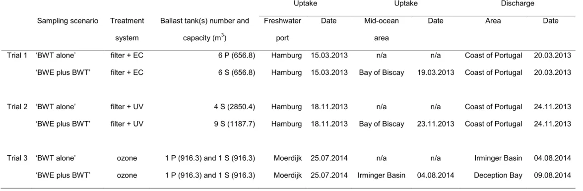
of ballast uptake in freshwater ports and mid-ocean areas and ballast discharge for three ship-based trials conducted. EC, UV, P, S and n/a, denote electrochlorination, ultraviolet radiation, port side of ship, starboard side of ship, and not
applicable, respectively.
Uptake Uptake Discharge
Sampling scenario Treatment system
Ballast tank(s) number and capacity (m3)
Freshwater port
Date Mid-ocean area
Date Area Date
Trial 1 ‘BWT alone’ filter + EC 6 P (656.8) Hamburg 15.03.2013 n/a n/a Coast of Portugal 20.03.2013 ‘BWE plus BWT’ filter + EC 6 S (656.8) Hamburg 15.03.2013 Bay of Biscay 19.03.2013 Coast of Portugal 20.03.2013
Trial 2 ‘BWT alone’ filter + UV 4 S (2850.4) Hamburg 18.11.2013 n/a n/a Coast of Portugal 24.11.2013 ‘BWE plus BWT’ filter + UV 9 S (1187.7) Hamburg 18.11.2013 Bay of Biscay 23.11.2013 Coast of Portugal 24.11.2013
Trial 3 ‘BWT alone’ ozone 1 P (916.3) and 1 S (916.3) Moerdijk 25.07.2014 n/a n/a Irminger Basin 04.08.2014 ‘BWE plus BWT’ ozone 1 P (916.3) and 1 S (916.3) Moerdijk 25.07.2014 Irminger Basin 04.08.2014 Deception Bay 09.08.2014
Table 2. Alternative linear mixed effect models fitted to data, where y~log10 (abundances in ‘BWT alone’/abundances in
‘BWE plus BWT’) is the dependent variable, which is dimensionless, and T~log10 (abundances in ‘BWT alone’) is a covariate. Zooplankton and phytoplankton abundances were measured in management scales (i.e., m-3 and mL-1, respectively). Here, c, ɛ denote the intercept and residuals, respectively.
Alternative Models Description
y ~T + (1|Ship) + c + ɛ; T non-nested with plankton type (ZorP) as a factor.
Fixed Effects: T, c; Random Effects: Ship; Repeated Measures: Time.
y ~ T (ZorP) + (1|Ship) + c + ɛ T(ZorP) denotes the plankton type (ZorP: Zooplankton or Phytoplankton)
nested within T as a factor.
Fixed Effects: T(ZorP), c; Random Effects: Ship; Repeated Measures: Time y ~ T(Time) + (1|Ship) + c + ɛ, T(Time) denotes the time-segment nested within T as a factor.
Fixed Effects: T(time), c; Random Effects: Ship; Repeated Measures: Time
Table 3. Results of alternative linear mixed effect models fitted to data such that y ~ log10 (abundances in ‘BWT alone’/abundances in ‘BWE plus BWT’), which is dimensionless, and T ~ log10 (abundances in ‘BWT alone’) as a
covariate, with non-nested (model 1), nested with plankton type (ZorP) as a factor (model 2), and nested with Time as a factor (model 3). Time was considered as a repeated measure. Zooplankton and phytoplankton abundances were
measured in management scales (i.e., m-3 and mL-1, respectively). The results of random effects due to Ship and ZorP as factors are not presented, as those effects were redundant. Here, c, ɛ, FE, and RM denote intercept, residuals, fixed effects, and repeated measures, respectively, while est, var, stde, AIC, Coef, LB, and UB denote estimates, variance, standard error, Akaike Information Criteria, coefficients, lower bound, and upper bound. * denotes significant difference at 95% level.
Alternative Models
Fixed effects Repeated measures AIC
Est p-value F(t*), df 95% CI LB and UB Var Var stde
y ~ T + c + ɛ FE: T
c
0.000 0.009
35.3, 16,1 8.9, 16,1
44.90
Coef: T 0.88 0.000 *5.9, 16 0.57, 1.20
RM:
C Time
-0.91 0.009 *-2.9, 16 -1.56, -0.27
0.67 0.24
y ~ T(ZorP) + c + ɛ FE: T(ZorP) 0.000 18.7, 16,2 46.25
:ZorP-nested c 0.007 9.7, 16,1
Coef: T(P) 0.87 0.000 0.56, 1.18
RM:
T(Z) c Time
1.06 -1.03
0.001 0.007
0.50, 1.63 -1.73, -0.33
0.64 0.23 y ~ T(Time) + c + ɛ
:Time-nested
FE: T(Time) c
0.000 0.007
12.8, 16,3 9.5, 16,1
47.96
Coef: T(Time1) 0.95 0.000 *4.8, 16 053, 1.37
RM:
T(Time2) T(Time3) c
Time
0.94 0.74 -0.92
0.000 0.002 0.007
*4.8, 16
*3.7, 16
*-3.1, 16
0.53, 1.36 0.31, 1.17 -1.55, -0.29
0.63 0.22
Figure Legends
Fig. 1 Graphical comparison of plankton abundance in 'BWT alone' against 'BWE plus BWT' trials. Solid lines are given by fixed effect model, y ~ T + c + ɛ, where y ~ log10
(abundances in ‘BWT alone’/abundances in ‘BWE plus BWT’). On the panel (a) y ~ T(ZorP) + c + ɛ, where plankton type ZorP is nested within T ~ log10 (abundances in
‘BWT alone’). Dashed lines indicate the nested fixed effect regression lines given for Z and P. On the panel (b) y ~ T(Time) + c + ɛ, where Time is nested within T. Dashed lines indicate the nested fixed effect regression lines given for Times of data collection. Time was considered as a repeated measure. Zooplankton and phytoplankton abundances were measured in management scales (m-3 and mL-1, respectively).