Combined Faculties for the Natural Sciences and for Mathematics of the Ruperto-Carola University of Heidelberg, Germany
for the degree of Doctor of Natural Sciences
presented by Diplom-Physicist: Lothar Keck
born in: Maulbronn
Oral examination: 21st November, 2001
of stable isotope records from Alpine ice cores
Referees: Prof. Dr. Ulrich Platt
Prof. Dr. Konrad Mauersberger
Stable water isotope records (δ O and δD) of three down to bedrock ice cores from Monte Rosa massif (Swiss Alps) were evaluated in view of potentially recorded temperature signals.
On-line measurements of δD by a novel water reduction method yield an accuracy of 0.7 ‰.
Upstream effects in δ18O ice core records, assessed from recent surface composition and modelled backward trajectories, may decrease the 20th century trend by a factor of three. The comparison of δ18O records with 240 years of instrumental growing season temperatures indicates that major decadal and centennial temperature changes are concurrently recorded with a ∆δ18O/∆T relation of 1.7 ‰/°C. Decadal means of growing season isotope temperatures indicate that recent levels are the highest, though not unprecedented within the last millennium. The unparalleled respective minimum occurred around 1340 A.D. with decadal means of more than 1°C below the recent level. The three cores exhibit an isotopically depleted basal layer. Contrary to the hitherto assumption of their Pleistocene origin, a new hypothesis is introduced that explains these signals as a consequence of the rapid deformation of glacier ice near bedrock.
Klimatische Aussagekraft der stabilen Wasserisotopomere in Alpinen Eisbohrkernen
Tiefenprofile der stabilen Wasserisotopomere (δ18O und δD) dreier tiefer Eisbohrkerne vom Monte Rosa Massiv (Schweizer Alpen) wurden im Hinblick auf möglicherweise aufgezeichnete Temperatursignale ausgewertet. Durch eine neuartige Methode der Wasserreduktion sind On-line δD Messungen mit einer Genauigkeit von 0.7 ‰ möglich.
Upstream-Effekte in den δ18O Profilen, abgeschätzt aus der gegenwärtigen Zusammensetzung der Gletscheroberfläche und modellierten Rückwärtstrajektorien, können die Trends des 20.
Jahrhunderts um einen Faktor drei vermindern. Der Vergleich von δ18O Profilen mit instrumentellen Sommertemperaturen über 240 Jahre zeigt, daß Temperaturtrends über eine Zeitskala von Jahrzehnten bis Jahrhunderten übereinstimmend aufgezeichnet sind, wobei die Empfindlichkeit ∆δ18O/∆T etwa bei 1.7 ‰/°C liegt. Die derzeitigen mehrjährigen Mittel der Isotopentemperatur sind mit die wärmsten innerhalb des vergangenen Jahrtausends. Das beispiellose Temperaturminimum um 1340 A.D. weist um mehr als 1°C niedrigere mehrjährige Mittel der Isotopentemperatur auf. Alle drei Kerne zeigen eine isotopisch leichte basale Schicht. Im Gegensatz zu der bisherigen Annahme ihres eiszeitlichen Ursprungs wird eine neue Theorie aufgestellt, welche diese Signale als Folge der schnelleren Eisdeformation in Felsbettnähe erklärt.
1. INTRODUCTION... 10
2. STABLE WATER ISOTOPES IN PRECIPITATION... 17
2.1 FRACTIONATION PROCESSES... 17
2.2 FORMATION OF PRECIPITATION... 17
2.2.1 Equilibrium condensation... 17
2.2.2 Kinetic effects ... 18
2.2.3 Sub-cloud effects... 20
2.3 GENERATION OF ATMOSPHERIC WATER VAPOUR... 20
2.4 VARIABILITY IN ALPINE PRECIPITATION... 21
2.4.1 Seasonal variations and altitude effect ... 21
2.4.2. Long term ∆δ18O/∆T -relations... 24
3. METHODS ... 26
3.1 CORE DRILLING AND PROCESSING... 26
3.2 HYDROGEN ISOTOPES... 27
3.2.1 Principle of the H/Device ... 28
3.2.2 Adaptation of the method to the MAT 230C mass spectrometer... 28
3.2.3 Effects of apparative parameters ... 29
3.2.4 Precision ... 32
3.2.5 Memory effect ... 32
3.2.6 Calibration ... 32
3.2.7 Standard drift... 33
3.2.8 Overall Reproducibility ... 33
3.2.9 Summary ... 34
3.3 OXYGEN ISOTOPES... 34
3.4 STABLE ISOTOPE INTERCOMPARISIONS... 34
4. GLACIOLOGICAL FEATURES... 36
4.1 STEADY ICE FLOW... 36
4.1.1 Ice deformation... 36
4.1.2 Flow models for CG... 38
4.2 MASS BALANCE... 39
4.2.1 Background... 39
4.2.2 Mass balance measurement ... 40
4.2.3 Results and discussion ... 43
5. DATING... 45
5.1 STATE OF THE DATING... 45
KCS... 45
KCH ... 48
CC... 48
CC... 51
5.3 SUMMARY... 54
6. SAMPLING TRAIT... 56
6.1 RECORDED SEASON... 56
6.1.1 Melt events... 56
6.1.2 Wind erosion... 58
6.1.3 Seasonal variations in precipitation amount ... 59
6.1.4 Application on ice core records... 61
6.2 RECORDED WEATHER TYPES... 64
6.2.1 Precipitation amount ... 64
6.2.2 Fresh snow samples ... 65
6.3 SUMMARY... 68
7. STABLE ISOTOPE LONG TERM RECORDS ... 69
7.1 DATED SEQUENCES... 69
7.2 SYSTEMATIC UPSTREAM EFFECTS... 72
7.2.2 Backward trajectories... 72
7.2.2 Shallow cores... 74
7.2.3 Result ... 76
7.2.4 Summary and discussion... 77
7.3 COMPARISON WITH INSTRUMENTAL RECORDS... 78
7.3.1 Site specific temperature series ... 78
7.3.2 Qualitative comparison ... 79
7.2.4 Sensitivity of the stable isotope thermometer... 82
7.4 A MILLENNIUM OF ISOTOPE TEMPERATURES... 83
7.5 COMPARISON TO OTHER MILLENNIAL RECORDS... 85
7.5.1 Oscillations of Glaciers ... 85
7.5.2 Tree-rings ... 85
7.6 SENSITIVITY... 87
7.6.1 The restriction on the growing season... 87
7.6.2 The high elevation ... 87
7.6.3 Climate induced changes in the ice core seasonal composition ... 91
7.6.4 Climate induced changes in precipitation types ... 91
7.6.5 Summary ... 91
7.7 REMARKS ON THE D-EXCESS... 92
7.8 SUMMARY... 92
8. BASAL LAYER ISOTOPE SIGNALS ... 94
8.1 RELATION TO OTHER SITES... 94
8.2 PLEISTOCENE ICE... 96
8.2.1 Trace gases in air bubbles ... 96
8.2.2 Other potential age constraints ... 98
8.3 SOURCE REGION ANOMALY... 98
8.3.1 Mass flow rates ... 100
8.3.2 Isotopic composition ... 100
8.4.5 Suggested process... 107
8.4.6 Predicted effect on isotope profiles... 107
8.4.7 Relation to Ion content... 112
8.5 SUMMARY AND OUTLOOK... 113
REFERENCES ... 115 ANNEX A: CORE META DATA...I ANNEX B: UPDATED VOLCANO CHRONOLOGY... II ANNEX C: RADIONUCLIDE INVENTORIES ... V C.1 BACKGROUND... V C.1.1 The natural radioisotopes 10Be and 210Pb ...V C.1.2 The artificial radioisotopes 137Cs and Tritium ... VII C.2 METHODS... VIII C.3 RESULTS... IX ANNEX D: GLACIER SIMULATOR EXPERIMENTS ... XI D.1 PRODUCTION OF HOMOGENEOUS POLYCRISTALLINE ICE... XI D.2 DESIGN AND OPERATION OF THE GLACIER SIMULATOR... XI D.3 RESULTS AND DISCUSSION... XIII
Drill sites
CDD Col du Dome, Mont Blanc massif CDL Col du Lys, Monte Rosa massif CG Colle Gnifetti, MonteRosa massif Ice cores
CC Down to bedrock core at Colle Gnifetti
KCH do.
KCS do.
Institutes
DISAT Dipartimento di Scienze dell’ Ambiente e del Territorio, Milano DISGAM Dipartimento di Scienze Geologiche, Ambientali e Marine ETHZ Laboratory of Hydraulics, Hydrology and Glaciology, Zurich IUP Institut für Umweltphysik, Heidelberg
LGGE Laboratoire de Glaciologie et Geophysique de’l Environnement, St. Martin d’ Heres
LMCE Laboratoire de Modélisation du Climat et de l'Environnement, Saclay ZAMG Central Institute for Meteorology and Geodynamics, Vienna
Analyses
CFA Continuous flow analyses
ECM Electric conductivity measurement
IC Ion chromatography
MS Mass spectrometer
Other
ALPCLIM EU project: “Environmental and Climate Records from High Elevation Alpine Glaciers”
IAEA International Atomic Energy Agency SSA Singular spectrum analyses
1. Introduction
Environment and climate have always strongly affected the fate of man. Nowadays in turn human activities may cause climate change because the radiation balance of the earth is affected by anthropogenic trace gases and aerosols which were intensely produced since the beginning of the industrial era (Shine et al. 1990). Thus there is need to asses any potential influence of human activities on climate against the past natural variability. Assuming model derived natural fluctuations the global warming in the second half of the 20th century is most probably already attributable to the human influence (Tett 1999). However, global instrumental observations cover at best the last 150 years with respect to air temperature and only a few decades with respect to atmospheric trace gases and aerosols. Therefore temporal and spatial patterns of the natural variability in climate and geochemical cycles, as well as their interactions, can only poorly be estimated from instrumental records.
To extent the time range of atmospheric records various types of natural climate archives, as sediments, trees and glaciers, can be exploited. The most comprehensive records are obtained from ice cores of “cold” glaciers. Such glaciers are characterised by ice temperatures well below the pressure melting point and thus the records are not blurred by meltwater percolation. The use of the stable water isotope (H2 18O or HDO) content of the ice matrix as temperature proxy is well established (Dansgaard 1973). Concurrent measurements of H2 18O and HDO providing the secondary quantity deuterium-excess may can give insight into the water vapour source region of the stored precipitation (Barlow et al. 1993). Moreover the atmospheric aerosol load is recorded in the impurity content of the ice and atmospheric gases are trapped in air bubbles.
Deep ice cores from polar ice sheets yielded fundamental new insight in the climate system.
The most outstanding results are currently the reconstruction of 420.000 years of isotope temperature and atmospheric trace gase composition from the Vostok ice core, Antarctica (Petit et al. 1999) and high resolution records of one full glacial-interglacial cycle from the GRIP (Dansgaard et al. 1993) and GISP2 (Stuiver and Grootes 2000) ice cores, central Greenland. However, while these two Greenland records show close agreement in isotope pattern for the Holocene and most part of the Wisconsin glaciation, significant differences in the lower core sections spanning the Eemiam interglacial and the penultimate glaciation remain until now unexplained (Grootes et al. 1993).
The success of polar ice core studies motivates the investigation of ice cores from alpine1 glaciers to access the potentially conserved most valuable mid- and low latitude climate records. Specifically the European Alps are most intriguing for ice core studied for two reasons:
1 Note that “alpine” is used for high mountains in general, whereas “Alpine” refers to the European Alps
• In contrast to all other ice core sites, a dense network of instrumental meteorological records in the European Alps and adjacent regions over more than 250 years is available.
This offers the unique possibility of a mutual validation of ice core climate proxies and instrumental long term records.
• Due to the comparably short life time of atmospheric particles the anthropogenic change in aerosol load and its possible impact on climate is concentrated on industrialised areas.
Thus ice core records from cold Alpine glaciers are particular due to their location within major antropogenic source areas.
However, Alpine cold glaciers exist solely in the high elevation summit regions, since only there the mean annual air temperature (MAAT) is low enough. As a consequence, Alpine drill sites have several peculiarities as pointed out by Wagenbach (1992):
• Due to their exposed location on small scale glaciers in the summit regions, they are subject to strong wind erosion of snow. As the extend of wind erosion depends on meteorological conditions and surface geometry, it is spatially and seasonally variable.
Consequently, the finally conserved fraction of annual precipitation may reflect a strongly seasonally weighted atmospheric signal.
• The high altitude aerosol concentration is controlled by the seasonally variable intensity of vertical mixing. Therefore the seasonal amplitudes of aerosol concentrations are always large compared to their long term trends. This applies also to the stable isotopes in mid- latitude precipitation. As a result, long term trends of stable water isotopes or aerosol related records derived from alpine ice cores are very sensitive to any changes in the conserved fraction of annual precipitation.
• Due to the local sources of trace substances and water vapour, the seasonally variable vertical mixing intensity is expected to cause seasonal variations in the spatial representativity of Alpine ice core records.
• The conserved fraction of annual precipitation generally undergoes systematic spatial changes at the glacier surface. Due to the inflow of ice from upstream the drill site, temporal trends from alpine ice cores are superimposed by the spatial variations along the surface. Such upstream effects are to be taken into account even if the core is drilled at a saddle point (Wagner 1996).
• Cold alpine glaciers in the summit regions are of irregular topography, with the horizontal extension being comparable to glacier thickness. Particularly in the proximity to bedrock this causes a complex ice flow pattern and a strongly non-linear age-depth relation. Due to the annual layer thinning seasonal signals in aerosol concentrations can not be resolved in the lower core sections. Thus the dating of the major parts of the time range remains a challenge.
The EU-project ALPCLIM (Environmental and Climate Records from High Elevation Alpine Glaciers) was devoted to the exploitation of Alpine ice cores for climate related record. It was launched in 1998 and coordinated by the Institut für Umweltphysik (IUP), Universität
sites indicated in Figure 1.1:
• Colle Gnifetti (CG, located in the Monte Rosa massif)
• Col du Lys (CDL, as well Monte Rosa massif)
• Col du Dome (CDD, Mont Blanc massif)
Figure.1.1: Dots: Location of the main ALPCLIM drill sites Colle Gnifetti and Col du Lys at Monte Rosa (45° 56’ N, 7° 52’ E) and Col du Dome at Mont Blanc (45° 50’ N, 6° 50’ E).
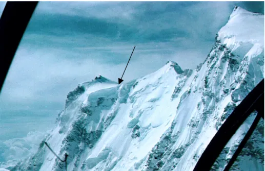
The main concern of this thesis are the ice cores from CG, a small firn saddle situated at 4450 m asl. As illustrated in Figure 1.2, CG is located in an extremely exposed location. Therefore strong wind erosion causes an extraordinary low annual accumulation of snow. As a result, CG is the unique Alpine key site to recover long term ice core records. Accordingly CG is glacialogically well characterised (Alean et al. 1984) and was subject to ice core studies and related work since the 70ties (Oeschger et al. 1977). However, the specific problems of Alpine drill sites apply in particular for CG.
Figure 1.2: View of Colle Gnifetti (indicated by the arrow) from north. The three summits of Monte Rosa range are (from left to right) Signalkuppe, Zumsteinspitze and Nordend.
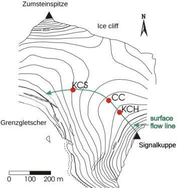
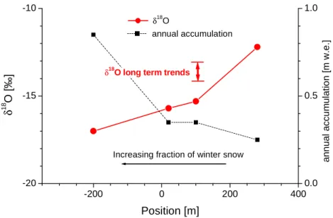
The shape of the saddle, being situated between Zumsteinspitze and Signalkuppe, is shown in Figure 1.3. The annual accumulation varies systematically from 0.1 m w.e.2 at the shadily north-west slope of Signalkuppe to more than 1.2 m w.e. at the sunny south slope of Zumsteinspitze, where the formation of ice layers effectively protects the snow from wind erosion (Alean et al. 1983). The wind erosion affects preferably the isotopically light dry winter snow (Wagenbach 1989). Thereby the systematic variation of annual accumulation is accompanied by a spatial variations of the mean stable isotope content, as illustrated in Figure 1.4. This spatial variations are large compared to Holocene stable isotope long term trends.
Thus, due to the potential upstream effects e.g. an increase of stable isotopes in the second half of the 20th century which had been observed in the “Chemie Core” (CC, drilled in 1982 at the position shown in Figure 1.3) can not unambiguously be attributed to a temperature signal. In fact the observed increase is much stronger than expected from the simultaneous warming trend in Alpine air temperatures.
2 m w.e. (meter water equivalent) is the thickness of a layer of snow or firn when compressed to the density of water. The unit is commonly used to account for the compaction of snow and firn.
4500 44
00 4500
I I
IIII III
I
II II II I
II I I I I I I III I II I I I IIIII II I I II II I
I
Zumsteinspitze
Signalkuppe Signalkuppe Ice cliff
Grenzgletscher
Figure 1.3: Surface topography of CG. The deep cores KCH and KCS (drilled in 1995) and CC (drilled in 1982) are aligned approximately along a surface flow line.
The annual accumulation of snow is also strongly affected by surface topography. The topography is changed by wind action and potentially by glacier flow. This causes both quasi- random spatial variations of the annual net snow accumulation and systematic temporal variations in annual snow accumulation at fixed location. Such variations in annual accumulation in ice cores from CG have been reported by Armbruster (2000). A systematic increase of annual accumulation with air temperature was suggested by Schotterer et al.
(1978). The presence of non steady state conditions at Colle Gnifetti is also supported by photos showing visible changes of the surface topography at the ice cliff and at the rock outcrops in the slope of Signalkuppe during the last decades (Wagenbach pers. com.). On the other hand, a digital comparison of a photograph taken in 1883 with a recent one taken from the same position shows no discernible changes for the bulk surface topography (Wagner 1996). In any case, potential temporal changes in surface topography are a matter of concern as the annual snow accumulation and as shown in Figure 1.4 also the stable isotope content would be affected.
-200 0 200 400 -20
-15 -10
δ18O
δ18 O [‰]
Position [m]
0.0 0.5 1.0
Increasing fraction of winter snow annual accumulation
δ18O long term trends
annual accumulation [m w.e.]
Figure 1.4: Spatial variations of annual accumulation and surface isotopic composition between Zumsteinspitze (at position - 350 m), saddle point (at 0 m) and Signalkuppe (at + 400 m)
The useful time scale in ice cores from CG covers at least several centuries (Schäfer 1995).
However, the basal layer section of cold Alpine glaciers, which is expected to contain the major part of the conserved time range, has not yet been dated. Flow models suggest an age of a few thousand years for the basal ice (Wagner 1996) whereas stable isotope anomalies hint at potential remnants of Pleistocene ice (Wagenbach 1993). This would be in agreement with the time horizon of alpine ice core records from the Tibetan Plateau (Thompson et al. 1997) and the Andes (Thompson et al. 1998), from where climate and environmental records back into the last glacial stage are reported. To exploit the unique climate records of CG, two down to bedrock cores (KCH and KCS) were drilled in 1995 by IUP in collaboration with Physikalisches Institut, Universität Bern (PIUB). As displayed in Figure 1.3, these cores are approximately on a surface flow line with the already existing and completely analysed core CC from 1982.
Within ALPCLIM, one core was recovered at Colle de Lys (CDL), situated at 4150 m asl in the southern part of the Monte Rosa massiv and only 1 km from CG by the Dipartimento di Scienze dell’Ambiente e del Territorio (DISAT), Milano. As the annual snow accumulation is relatively well preserved at CDL, the record is of seasonal resolution though covering only the last three decades.
Finally, an ice core from Col du Dôme (CDD), situated at 4250 m asl in the northern part of the Mont Blanc summit range, was available. The core thence had been drilled and mainly analyses by the Laboratoire de Glaciologie et Géophysique de l’Environnement (LGGE). The accumulation rate is comparable to CDL and thus also here ice core records in sub-seasonal resolution could be obtained over 80 years, approximately.
records, the inventories of the radionuclides 10Be, 210Pb, 3H and 137Cs, each with a relatively well known spatial and temporal pattern of source and transport, were measured for each core.
Moreover, within ALPCLIM Alpine temperature series back to 1760 A.D. had been collected, homogenised and gridded (Böhm et al. 2000) by the Zentralanstalt für Meteorologie and Geodynamik (ZAMG), Vienna. Furthermore for each drill site a detailed recent climatological characterisation was established by ZAMG as well. Additionally, englacial temperature profiles as a potential additional temperature proxy in the Alpine region were evaluated by Laboratory of Hydraulics, Hydrology and Glaciology of ETH Zürich (ETHZ).
To assess climate records from the CG stable isotope long term records, the interpretation effort of this thesis focuses on the interconnected basic problems of Alpine ice core records:
• To assess their seasonal representativity of the ice records. This is mandatory both to compare of stable isotope records with instrumental time series and to estimate the spatial representativity of inherent temperature signals.
• To evaluate the influence of systematic upstream effects on stable isotope long term trends. This required intense field work for the drilling of supplementary shallow cores and the measurement of surface mass balance.
• To validate the ice core climate proxies by independent information from instrumental temperature series. In particular a direct calibration of the stable isotope thermometer is envisaged. The latter is a crucial point for the interpretation since the sensitivity of the stable isotope thermometer strongly depends on the location. This is concluded both by direct observations (Rozanski et al. 1997) and model studies (Cole et al. 1999). However, this requires a precise dating and an appropriate processing of the various data sets.
The validation of stable isotope trends from CG is attempted by comparing them with the respective results of the other ALPCLIM drill sites. On the base of these investigations the basic prospects of temperature proxies from Alpine ice core records can eventually be assessed.
A part of this work arose of the reflection on the basal ice at CG. While the light stable isotope values suggest pleistocene ice, the visual stratigraphy suggested an alternative explanation by the migration of water between ice grains into shear planes. This hypothesis on the origin of the main isotope signal in alpine ice cores is presented and discussed.
2. Stable water isotopes in precipitation 2.1 Fractionation processes
Besides the ordinary water molecule H2O of mass 18 amu, also small concentrations of the main heavy isotopomeres HDO and H218
O participate in the hydrological cycle. The variations of HDO and H218
O concentrations are controlled by the fractionation during evaporation and condensation. With R1 and R2 being the isotope ratio in phase 1 and phase 2 (R= [H218O]/[H2O] or R= [HDO]/[H2O], respectively) the fractionation factor is defined as:
2 1
R
= R α
A measure for the degree of fractionation is ε, defined as ε = α - 1. Because the absolute isotope ratios R are hard to measure and in order to have a standardised scale, it is valuable to describe the isotopic composition of natural water bodies on the δ-scale versus V-SMOW.
This δ-value in permille is defined as:
⋅1000
= −
−
−
−
SMOW V
SMOW V sample SMOW
V R
R δ R
V-SMOW is an artificial standard water with an isotopic composition being approximately equal to the Standard Mean Ocean Water (SMOW).
The fractionation at phase transitions is based on two physical processes:
1. Equilibrium fractionation: Since the vapour pressure of the heavier components is slightly lower, vapour is generally depleted in heavy isotope content compared to a liquid or solid phase in equilibrium.
2. Kinetic effects: Heavier isotopes exhibit a lower molecular diffusion coefficient. Thus they have to overcome a larger transfer resitance when passing through a laminar-viscose layer. As the equilibrium fractionation is much lower for H218
O, the variations in δ18O concentrations are proportionally more affected by kinetic effects than for δD. Kinetic effects, which occur both at the evaporation and condensation, are the main cause that the two isotopes do not behave completely analogous in the natural water cycle.
2.2 Formation of precipitation
2.2.1 Equilibrium condensation
During the cooling of an air parcel, the heterogeneous condensation of its water vapour content starts and is maintained at a very low supersaturation of a few permille. Thus kinetic
starts, the newly formed condensate is enriched in heavy isotopes while the remaining vapour is accordingly depleted. If the cooling proceeds and the condensed portion is removed from the air parcel, the remaining water vapour undergoes a successive depletion in heavy isotopes content and thus also the continuously newly formed condensate. The degree of the depletion is controlled by the remaining fraction of the initial water vapour content and thus by the temperature difference between initial dew point and actual temperature of the air parcel. This implies all the so-called isotope effects as there are seasonal-, latitude-, altitude-, inland-, the paleo-climatic effect (Dansgaard 1973) and the amount effect.
The so called “simple Raleigh condensation model“ assumes that the generation of liquid phase takes place in equilibrium and that the condensate is immediately removed from the cloud without any isotope exchange with the vapour. This simple Raleigh model is applicable only on clouds with low liquid water content. The model yields (Dansgaard 1964):
• The ∆δ18O/∆T -relation, in other words the sensitivity of the isotope thermometer with respect to the ambient temperature T, increases at low temperatures. Typical values are between 0.24 ‰ /°C (solid-liquid condensation and moist adiabatic cooling at 20°C) and 0.82 ‰/°C (vapour-solid condensation and isobaric cooling at 0°C).
• The slope ∆δD/∆δ18O is affected both by the instantaneous composition of water vapour and the temperature dependent fractionation factors. In the range of moderate atmospheric temperatures the effects counterbalance such that the slope is almost constantly 8 both for isobaric and adiabatic cooling ((2) → (3) in Figure 2.1). Thus the impact of non- equilibrium effects is reflected in the deuterium excess (D-excess or d), being defined as
O D
d =δ −8⋅δ18
2.2.2 Kinetic effects
The simple equilibrium Raleigh model with vapour-solid fractionation factors predicts a pronounced increase of the D-excess at polar temperatures ((3) → (4a) in Figure 2.1).
Contrary to that, only a gradual increase has been observed in polar snow ((3) → (4) in Figure 2.1). Moreover, the model predicted ∆δ18O/∆T –relation strongly exceeds the observations.
Model predictions and field data can be reconciled by taking into account kinetic effects at the formation of snow (Jouzel and Merlivat 1984).
-30 -20 -10
-200 -100 liquid or solid
vapour
(4a)
(2)
(3) (3a)
(4)
d=0 δ18O [‰]
δD [‰]
(1)
(SMOW)
MWL (d=10)
Figure 2.1: Variations of δ18O and δD in at evaporation and condensation. The D- excess (d) is the vertical distance to the straight line δD = 8⋅δ18O. MWL: meteoric water line.
(SMOW)→(1): Evaporation from the sea surface.
(1)→(2): condensation of water vapour at dew point (2)→(3): condensation at moderate temperatures (3)→(3a): evaporation of raindrops
(3)→(4a): condensation at low temperatures as predicted by equilibrium condensation (not observed) (3)→(4) condensation at low temperatures taking into account kinetic effects
More generally, at temperatures between the activation of ice nuclei and the homogeneous nucleation of water droplets, solid and liquid phase generally coexist in mixed cloud systems.
Since the saturation vapour pressure with respect to ice is lower than with respect to water, the ice crystals grow on the expense of the liquid droplets (Rogers 1989). During this so called Bergeron-Findesein process kinetic effects occur both at evaporation of droplets and at condensation on ice crystals. While for the δ-values this leads only to minor changes compared with the predictions of the vapour-solid kinetic model, it remedies instabilities for the predicted D-excess with respect to cloud vapour pressure history (Ciais and Jouzel 1994).
The δ-values and the D-excess in precipitation also depend on the temperature at which clouds switch from supercooled drops to ice particles. Therefore, also the microparticle load of an air parcel acting as freezing nuclei affect the isotopic composition of precipitation (Fisher 1991). However, contrary to the formation of polar precipitation in stratiform clouds it has been suggested that the stable isotopes in precipitation from deep convective clouds are almost unaffected by the Bergeron-Findesein process (Federer et al. 1982).
The process of supercooled liquid water droplets in clouds being captured by ice particles is called riming. Case studies indicate that depending on the vertical air motion in clouds riming
parts of the cloud (Fujiyoshi et al. 1986). Correspondingly the stable isotope values of rimed particles may over- or underestimate the mean cloud condensation temperature.
2.2.3 Sub-cloud effects
Raindrops may undergo a significant shift in their isotopic composition between cloud base and ground due to evaporation and isotopic exchange with ambient water vapour. As indicated in Figure 2.1 (3)→(3a) sub-cloud evaporation increases the δ-values and due to the kinetic effects it lowers the D-excess of precipitation (Ehhalt et al. 1963). In contrast to raindrops the effect of evaporation on the isotopic composition of snow flakes is negligible due to the low molecular diffusion rates in ice.
2.3 Generation of atmospheric water vapour
Both equilibrium fractionation and kinetic effects occur at the evaporation of water vapour from sea surface or lakes (Ehhalt and Knott 1964). The isotopic composition of the evaporating water vapour net flux depends on the local meteorological conditions temperature, humidity and wind speed. Moreover, due to the atmosphere-sea isotope exchange, it is also affected by the isotope ratio of the already existing vapour in the marine boundary layer (Craig and Gordon 1965). Assuming a global closed system, it can be shown that the D-excess in atmospheric water vapour increases with decreasing relative humidity h and increasing sea surface temperature SST (Merlivat und Jouzel 1979). For a relative humidity of 70 – 80 % and a SST of 20 – 25 °C, average values for the subtropical evaporation belts, the model predicts a D-excess of ≈ 10 ‰ ((SMOW) → (1) in Figure 2.1).
In fact this value resembles the present day global average of the D-excess in precipitation. As the subsequent formation of precipitation does frequently hardly affects the D-excess, most meteoric water bodies are close to the meteoric water line (MWL, see Figure 2.1):
δD = 8⋅δ18O + 10
In agreement with the model a high D-excess occurs in areas of evaporation at low humidity, such as the eastern Mediterranean (Gat and Carmi 1970). However, the theoretically presupposed closure equation does not hold on a local scale (Jouzel and Koster 1996).
At continental sites the re-evaporation of precipitation from plants, soil and surface waters particularly in summer may be a significant contribution to the local water vapour (Koster et al. 1993, Jakob and Sonntag 1991). Whereas the evaporation from land surface and in particular plant transpiration acts mainly without fractionation (Knott 1964, Zimmermann 1967), kinetic effects at the evaporation of meteoric surface waters can cause an enhanced D- excess in precipitation at the luv side of large lakes (Gat et al. 1994).
2.4 Variability in Alpine precipitation
The actual isotopic composition of water vapour in an air parcel reflects its history of condensation and admixture of fresh water vapour. Moreover, the relation between condensation temperature and surface temperature depends on the weather type. Accordingly the variable synoptic weather types cause a poor correlation of stable isotopes and local surface temperature for single precipitation events. However, monthly or annual means of stable isotopes in precipitation at a given point represent the average from a variety of precipitation events.. As this tends to average out the effects from different air mass histories, a positive correlation both for monthly (i.e. seasonal) and annual means in δ18O and local temperature is found for most mid- and high latitude sites (Rozanski et al. 1982). These temporal means are controlled by the spatial and temporal pattern of air mass trajectories and the precipitation-evapotranspiration history
2.4.1 Seasonal variations and altitude effect
δ-values show distinct seasonal variations in the Alpine region. The seasonal cycle of δ 18O from the four Swiss IAEA precipitation series (IAEA 1981) is displayed in Figure 2.2. Like the seasonal variations in temperature the monthly means exhibit a maximum in July and August. However, compared with the seasonal variations in temperature, the variations in δ18O exhibits a steeper decrease in autumn and a more gradual increase in spring
1 2 3 4 5 6 7 8 9 10 11 12
-15 -10 -5
δ18 O [‰]
month Bern (572 m asl.)
Meiringen (632 m asl.) Guttannen (1055 m asl.) Grimsel (1950 m asl.) average
Figure 2.2: Seasonal variations of δ18O in Alpine precipitation from Swiss IAEA stations based on the monthly means from 1971-1992. Except Bern all stations are located in the eastern Bernese Oberland.
raindrops preferably at the low altitude in summer was discussed by Siegentaler and Qeschger (1980). However, with the time series until 1992 according to Figure 2.2, neither the seasonal amplitude nor the shape of the cycle exhibits a systematic change with altitude. Moreover, since the percentage of solid precipitation increases with altitude the strength of a potential evaporation effect is expected to be of minor importance there. On the other hand, the ∆δ/∆T – relation predicted by a simple Raleigh model increases at low temperatures. Therefore the seasonal amplitude is expected to increase with altitude. The seasonal variations in δ 18O from the IAEA stations (altitude below 1850 m asl.) correspond to temporal seasonal ∆δ/∆T – relations of 0.33 – 0.54 ‰/°C (Rozanski et al. 1992). However, a value of 0.68 ‰/°C is reported from precipitation samples at Jungfraujoch (3580 m asl) (Schotterer et al. 1997). This suggests that in fact the seasonal amplitude increases with altitude.
Based on long term means an overall altitude effect of 0.2 ‰/100 m is reported for the Bernese Alps. This relation holds up to an altitude of 4000 m asl. (Stichler and Schotterer 2000). Taking this value of 0.2 ‰/100 m the mean seasonal variation from the IAEA data can be shifted to the altitude of CG (4500 m asl.). However, also a spatial shift in δ18O values is expected to occur between in the Bernese Alps and the Monte Rosa massif as they are located on different major orographic divides of the Alps. Moreover, the regional altitude effect could be different in the Monte Rosa massif since the altitude effect for individual precipitation events is stronger at the luv side of the Alps (Dray et al. 1997). Therefore the extrapolated seasonal variations are compared to site specific mean δ18O means.
1 2 3 4 5 6 7 8 9 10 11 12
-25 -20 -15
δ18 O [‰]
month Grenzgletscher
IAEA extrapolated
Figure 2.3: Seasonal variations of δ18O for the Monte Rosa massif at 4200 m asl. Solid: estimated from IAEA low level data and an altitude effects of 0.2 ‰/100 m. Dotted: monthly means from an ice core at Grenzgletscher.
25 fresh snow samples were collected in summer (middle of June to middle of September) 1998, 1999 and 2000 at Colle Gnifetti. They exhibit a mean δ18O of –13.6 ‰. This agrees well with the high altitude summer level estimated from the IAEA data shifted with the altitude effect of 0.2 ‰/100 m ( –14.1 ‰). The seasonal variations from IAEA data corrected on the altitude effects can also be compared to monthly δ18O means derived from an ice core at Grenzgletscher. This site is only 1 km from Colle Gnifetti at an altitude of 4200 m asl.
(Eichler et al. 2001). With an annual accumulation of 2.7 m w.e. this core may display the seasonal variations completely. However, these ice core derived monthly means suffer from the uncertain dissection in months. Figure 2.3 shows that the seasonal variations from IAEA data shifted to the altitude of 4200 m asl. agree fairly well with the seasonal variations from the ice core with the latter suggesting a slightly lower winter minimum.. As being supported from site specific data, the mean seasonal variations from the IAEA data set extrapolated to an altitude of 4500 m asl. will be used as a best guess for the seasonal variations of δ18O in precipitation at Colle Gnifetti.
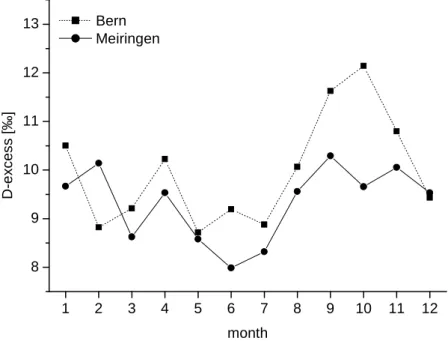
The seasonal variations of the D-excess in high altitudes are hard to estimate. Figure 2.4 shows the seasonal variation of the for low level stations. The maximum in autumn may be explained by the evaporation into dry polar air masses over the Atlantic ocean. The summer level (mid of June to mid of September) of 9.4 ‰ is well below the respective value from fresh snow samples of 13 ‰. The difference may partly be explained by the evaporation of raindrops in summer. However, it may also suggest a potential influence of local uplift of air masses on the D-excess. An increasing D-excess during solid-liquid condensation at low temperatures is expected. This would increase the D-excess mainly in winter.
1 2 3 4 5 6 7 8 9 10 11 12
8 9 10 11 12 13
D-excess [‰]
month Bern
Meiringen
Figure 2.4 Seasonal variation in D-excess at Alpine low level IAEA stations
∆δ ∆
The correlation of annual means in δ18O and surface temperature varies substantially even on a regional scale (Rozanski et al 1992). Rozanski et al. (1992) estimated long term ∆δ18O/∆T - relations from four Swiss IAEA stations to be 0.45 – 1.1 ‰/°C. Long term ∆δ18O/∆T - relations based on ice core records are discussed in detail in chapter 7.
The long term ∆δ18O/∆T –relation at a certain location could be strongly affected by continental water recycling as a significant portion of the variability in annual means of δ18O is caused by it (Koster et al. 1993). Specifically for summer precipitation in Alpine ice cores a strong effect of continental water recycling is expected since:
• The contribution of continental re-evaporation is more important in summer, as being reflected by the weak inland effect in Europe during this season (Knott 1964).
• The degree of local water recycling is expected to be relatively large in the Alps due to the persistence of local wind fields decoupled from the synoptic atmospheric circulation.
Specifically at clear sky conditions and flat pressure distributions, thermic wind fields develop (Barry 1981). This contribution of local evaporation causes a distinct diurnal variations in the humidity field of Alpine valleys (Hennemuth and Neureither 1986).
Evapo-transpiration of plants as the major part of continental evaporation acts mainly without fractionation. Therefore the shift of δ18O means due to continental water recycling is expected to be positive if the δ18O in groundwater is above the δ18O level of advected water vapour.
Typical δ18O values of Alpine groundwater and central European water vapour are displayed in Table 2.1.
Table 2.1: δ18O in groundwater and seasonal range of central European water vapour. The mean isotopic composition of the Rhone river is assumed to approximate the central Alpine groundwater.
water body δ18O [‰]
groundwater at northern margin of the Alps (Sonntag et al. 1979) -10
Rhone river (Schotterer et al. 2000) -14.5
Heidelberg water vapour summer level (Agemar et al. 2001) -15.3 Heidelberg water vapour winter level (dto) -20.9
The magnitude of the inland effect in precipitation for Europe suggests that the values for Heidelberg reflects the isotopic composition of water vapour advected to the Alps from west.
As δ18O in groundwater at the margin of the Alps is well above the values for advected vapour, evaporation from there is expected to increases the δ18O levels. However, due to the altitude effect the δ18O level in groundwater of Alpine valleys is much lower. As it is
comparable to the summer level of the advected vapour, the effect of evaporation from alpine valleys on the δ18O levels in summer is expected to be rather small.
3. Methods
3.1 Core drilling and processing
The two deep cores KCH and KCS were electromechanically drilled in October 1995. Core diameter is 3″ (≈ 7.5 cm). High resolution profiles of ECM (electric conductivity measurement) were established as a proxy for acid content. Density profiles were measured by gamma absorption at the Alfred-Wegener-Institut (AWI) in Bremerhaven. After that the cores were cut lengthwise using a band saw as shown in Figure 3.1. Additional shallow cores were drilled between 1998 and 2000 using a Sarbach 4″ (≈ 10 cm) drill driven by petrol engine. For these cores only the routine analyses of stable isotopes, ion content and partly liquid conductivity were performed.
16 43 16
52025
25 CFACFACFACFA
SI IC SI
Surface for ECM RI
Archiv
Figure 3.1: Sample cut pattern for the deep cores KCH and KCS. SI: stable isotopes, IC: ion chromatography and visual stratigraphy, RI: radioisotopes, CFA: continuos flow analyses.
An overview of the depth resolution for each sample type is given in Table 3.1. For the stable isotope samples the outer surface of the core was scraped off to eliminate potential effects of sublimation. The decontamination of the samples for chemical analyses was performed using an electric plane as described by Fischer (1997). Ion chromatography (IC) for Anions (Cl, NO3, SO4) and Cations (Na, NH4, K, Mg, Ca), accompanied by acidity analyses was performed and described by Armbruster (2000). Moreover, high resolution continuous flow analyses (CFA) was performed for NH4, Ca, liquid conductivity and particle content. Visual stratigraphy by means of digital image processing was done and described by Scholze (1998).
Additional microparticle analyses were performed by Saey (1998).
Table 3.1: Main data sets for the deep cores KCH and KCS.
Core KCH Core KCS
Analyses Resolution Depth range Resolution Depth range
Stable Isotopes 3.8 – 14 cm 0 – 48.5 m 5.6 – 20 cm 0 – 87.01 m
~ 2 cm 48.5 m – 60.35 m ~ 2 cm 87.01 m – 99.93 m Major Ions 5 - 10 cm
0 m – 28.75 m (Anions and Cations)
0 m – 60.35 m (only Anions)
5 – 10 cm 0 m – 42.39 m (Anions and Cations)
0 m – 99.93 m (only Anions) CFA (NH4, Ca,
liquid conductivity and particles)
~ 5 mm 28.75 m - 60.35 m ~ 5 mm 42.39 m - 99.93 m
ECM and density 2 mm Complete 2 mm Complete
Visual stratigraphy Complete Complete
3.2 Hydrogen Isotopes
To measure the deuterium content of ice, the melted sample has to be reduced to hydrogen gas. The D/H ratio of hydrogen is then measured with mass spectrometer (MS).
Reduction of water to hydrogen at the IUP was done before with hot zinc (Ehhalt 1963). For this work a new sample preparation method using hot chromium instead of zinc (Finnigan
“H/Device“) was established. The new method has the following promising advantages (Gehre et al. 1996, Brand et al. 1996):
• Good accuracy and precission.
• Small memory effect
• Due to the short reaction time it can be used as an online method, i.e. the hydrogen gas flows from the H/Device directly into the mass spectrometer. Thus there is no need of storing the hydrogen gas and an autosampler can be used.
• Chromium has the potential to form hydrogen gas not only from water but also from other hydrogen-bearing compounds, particularly methane.
• A very low amount of sample of less than 1 µl water (or the hydrogen equivalent of other substances) is sufficient for an analyses. This along with the previous item is of interest for the investigation of the carbon cycle at the IUP.
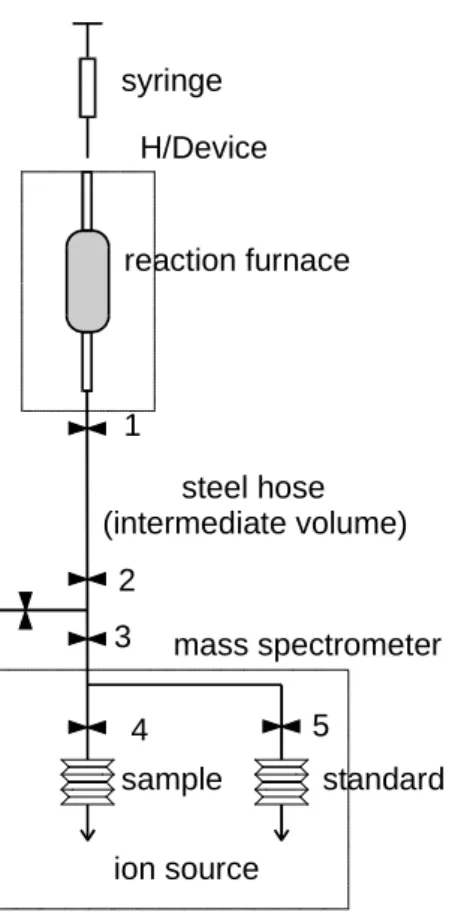
The essential components of the sample preparation are shown in Figure 3.2. 1-2 µl of water are injected with a gas-tight microsyringe through a septum into a reaction furnace filled with hot chromium powder. The water vapour formed by quantitative flash evaporation is then reduced (Gehre et al. 1996):
2 Cr + 3 H2O → Cr2O3 + 3 H2
during a certain “reaction time”. The reaction furnace is connected to the sample side of the dual inlet system of the mass spectrometer. When the reaction time is completed, valve 1 at the reaction furnace is opened. Then, during the “equilibration time“, the hydrogen gas is expanded into an “intermediate volume” mainly formed by a stainless steel hose which connects H/Device and MS. The furnace is closed (valve 1), valves 2, 3 and 4 are opened and the gas flows from the intermediate volume into the variable volume of the MS due to the pressure gradient. After a “transfer time“ the variable volume is closed (valve 4), compressed and the measurement by MS can be started. The furnace is evacuated until the next sample is injected during the “evacuation time”.
3.2.2 Adaptation of the method to the MAT 230C mass spectrometer
The H/Device is designed to be connected to recent Finnegan mass spectrometer types (MAT 252, DELTA S or DELTA PLUS). Since an older version (MAT 230C) was used for hydrogen analysis, two minor modifications of the H/Device were necessary:
1. The valves which were intended to be computer controlled had to be replaced by manually controlled ones.
2. A first test with the H/Device connected to the MAT 230C showed that the hydrogen pressure in the variable volume was far too low for an accurate analysis of the D/H ratio.
The pressure in the variable volume was increased to the required level by reducing the intermediate volume. For that the original steel hose (volume ≈ 92 cm3) was replaced with a much smaller one (volume ≈ 4 cm3).
1
2 3
4 5
H/Device
mass spectrometer
ion source steel hose (intermediate volume)
reaction furnace
standard sample
syringe
Figure 3.2: Sketch of the H/Device for online hydrogen isotope measurements
3.2.3 Effects of apparative parameters
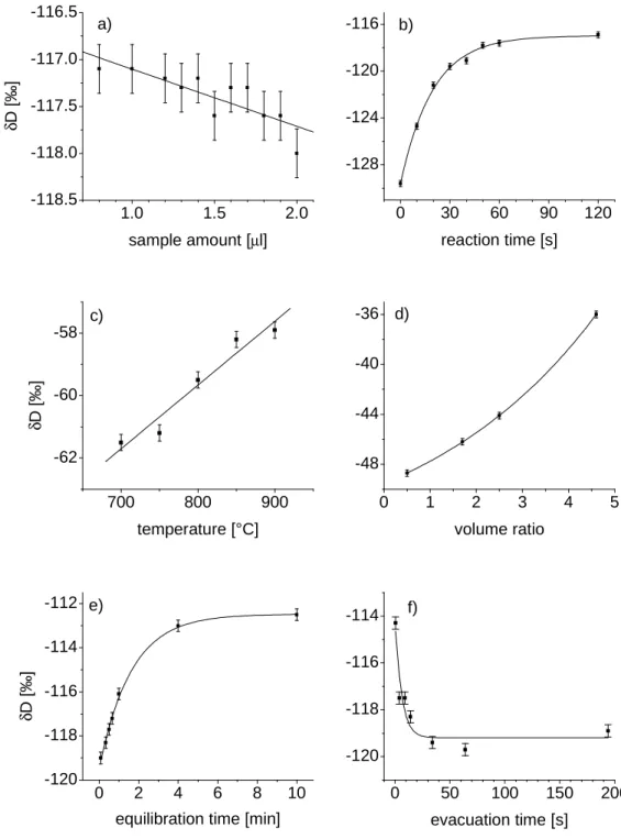
The zinc method reduces water samples almost quantitatively. However, δD values of samples prepared with the chromium method are several permille lower than δD values of the same samples reduced using the zinc method. This indicates that the reduction by chromium fractionates the hydrogen isotopes with the deuterium preferably remaining in the reaction furnace. It was investigated in which way this fractionation is affected by the different parameters of the analysis. The results affect the choice of the parameters for the routine analysis in view of a good precision of the method, since variations in these parameters are to some extend inevitable during manual operation. The effect of the various parameters on the measured δD value is shown in Figure 3.3. The not-varied parameters of the respective experiment are listed in Table 3.2.
1.0 1.5 2.0 -118.5
-118.0 -117.5 -117.0 -116.5
0 2 4 6 8 10
-120 -118 -116 -114 -112
0 30 60 90 120
-128 -124 -120 -116
0 50 100 150 200
-120 -118 -116 -114
0 1 2 3 4 5
-48 -44 -40 -36 a)
δD [‰]
sample amount [µl]
e)
δD [‰]
equilibration time [min]
b)
reaction time [s]
f)
evacuation time [s]
d)
volume ratio
700 800 900
-62 -60 -58
c)
δD [‰]
temperature [°C]
Figure 3.3: Effects of apparative parameters on the measured δD-value. The absolute values of δD for temperature and volume ratio are different to the others because other samples were used. Volume ratio means volume of reaction furnace over size of intermediate volume. To investigate the variation of temperature the sample was measured repeatedly. Otherwise the results would be biased by the effects of the evacuation time since changing the reaction time takes time. The transfer time had no effect on the measured values.
a) Sample amount
Sample amount does not critically affect the results. The lower limit is determined by the minimum pressure in the variable volume of the mass spectrometer which allows a measurement. This minimum pressure depends also on the state of the mass spectrometer.
b) Reaction time in the furnace
Trying reaction times as short as possible and observing the ion currents, practically performed by having valves 1, 2, 3 and 4 open at the injection (see Figure 3.3), indicated that the major part of the water is almost instantly reduced to hydrogen. However, a longer reaction time has the advantage that the measured δ-value is less affected by its variations.
c) Reaction temperature
The manufacture recommends an optimum reaction temperature of 850°C – 900°C for most compounds. However, for pure water the reduction basically works at temperatures almost down to 500°C. In the standard temperature range the measured δ-value increases only slightly with increasing temperature.
d) Size of the intermediate volume
The intermediate volume could be varied by expanding to valves 1, 2, 3 or 4. In Figure 3.3 the ratio of volume of reaction furnace over volume of intermediate volume is shown in order to suggest that the volume of different reaction furnaces should also affect the results.
e) Equilibration time and
f) Evacuation time of the furnace since the last sample
Varying equilibrium and evacuation time shows that the H- isotopes escape the furnace faster and that they are also preferably removed during the evacuation step. The values finally chosen for the routine analyses as shown in Table 3.2 are a compromise between time efficiency and the variations during manual operation not being critical for the measured values.
Table 3.2: H/Device parameters for the routine analyses. (1): according to present sensitivity of the spectrometer, of course to be kept constant within one run. (2): Minimum determined by the duration of the mass spectroscopic measurement. (3): proposed by manufacturer
Parameter value for routine analyses sample amount 1.2 – 1.72 µl (1) temperature of the furnace 850 °C (3) reaction time in the furnace 60 s intermediate volume ~ 6 cm3
equilibration time 30 s
transfer time 30 s
evacuation time 6.5 min (2)
Precision was determined by successive injections of the same sample. The mean standard deviation from five series of each four subsequent injections was 0.26 ‰. This excellent value agrees very well with the value of 0.24 ‰ determined by the manufacturer.
3.2.5 Memory effect
Having no memory effect was one of the promised advantages of the chromium method (Brand et al. 1996, Össelmann pers. com). Contrary to that a memory effect of 0.35 ± 0.09 % during 4 tests in February 1998 and 0.94 ± 0.57 % during 5 tests in January 2000 was found (% means permille difference between first and second measurement of the sample per 100 permille difference to the sample before). During all these tests the needle of the syringe was purged several times prior to the injection to remove the water which was potentially remaining in the syringe. The two results are significantly different at a t-test level of 97%. A potential reason for the inconstant memory could be an increasing amount of water remaining in the syringe as the syringe gets worn off. A memory effect probably mainly caused by the syringe is also reported by several other laboratories (Stievenard, pers. com. 1999, Steig pers.
com. 1999, Nelson pers. com. 1999). Also different qualities of the chromium powder and the formation of a surface coating from chromium vapour in the intermediate volume may contribute to the memory effect.
3.2.6 Calibration
Isotope ratios are measured with the mass spectrometer versus a hydrogen gas working standard (“δprst“) using the double inlet system. These δprst results have to be calibrated with respect to the δ-scale versus V-SMOW (“δSMOW “). As mentioned, the chromium reduction fractionates the hydrogen isotopes and the fractionation depends on the volume of reaction furnace and potentially state of the chromium filling. Since the specifications of furnaces and chromium are not generally constant, a day to day calibration by liquid standards is necessary.
For the calibration of the day to day laboratory liquid standards they were measured repeatedly versus the IAEA standards V-SMOW, GISP and SLAP within one run. The δSMOW
values of the laboratory standards were calculated from a linear fit through V-SMOW and SLAP (which define the δSMOW –scale). The accuracy of the fit can be checked by calculating δSMOW (GISP) from it. It yielded δSMOW (GISP) = 189.5 ± 0.1 ‰ which does excellently agree with the accepted value of –189.73 ‰ (IAEA 1995). The day to day calibration was then performed by measuring 2-3 laboratory liquid standards repeatedly. The δSMOW values of the samples are calculated from a linear fit through the laboratory standards. As samples and reference material are treated identically, this procedure is in full agreement with the “IT- principle”. The importance of this principle was outlined by (Werner and Brand 2001).
3.2.7 Standard drift
Since the day to day calibration relies on liquid standards, a potential standard drift due to evaporation or exchange with ambient water vapour deserves special attention. The drift rate can be estimated to be about 1 ‰ per 100 measurements from comparing δD of three intentionally frequently opened and measured samples with δD of a backup. Thus for a envisaged maximum drift of 0.3 ‰ after about 30 injections a new aliquot of the standard should be taken from the storage bottle. However, this value refers to 20 ml flasks with wide neck and no care being given to avoid partly evaporated drops getting back in the flasks by the needle of the syringe or the top. In the meanwhile more suitable flasks with narrow neck are used for the working standards and after the respective test the number of injections made by one aliquot of standard may be increased. Alternatively, flasks closed by a septum for the standards could be used.
3.2.8 Overall Reproducibility
A standard which is not used for the day to day calibration (“Alpen 2“) was treated and measured as an ordinary sample for 18 months since September 1999. Figure 3.5 shows the respective performance chart.
1 Sep 1 Jan 1 May 1 Sep 1 Jan
-96 -94 -92 -90 -88
δD [‰]
Figure 3.4: Performance chart for δD values of the “Alpen 2” standard since September 1999. The horizontal line and the grey area indicate average and standard deviation.