Break Date Estimation for VAR Processes with Level Shift with an Application to Cointegration Testing

BREAK DATE ESTIMATION FOR VAR PROCESSES WITH LEVEL SHIFT

WITH AN APPLICATION TO COINTEGRATION TESTING

P

EEENNNTTTTTTIII

S

AAAIIIKKKKKKOOONNNEEENNN University of Helsinki

H

EEELLLMMMUUUTTT

L

ÜÜÜTTTKKKEEEPPPOOOHHHLLL

European University Institute, Florence and

Humboldt University Berlin

C

AAARRRSSSTTTEEENNN

T

RRREEENNNKKKLLLEEERRR Humboldt University Berlin

In testing for the cointegrating rank of a vector autoregressive process it is impor- tant to take into account level shifts that have occurred in the sample period+There- fore the properties of estimators of the time period where a shift has taken place are investigated+The possible structural break is modeled as a simple shift in the level of the process+Two alternative estimators for the break date are considered, and their asymptotic properties are derived under various assumptions regarding the size of the shift+In particular,properties of the shift date estimators are obtained under the assumption of an increasing or decreasing size of the shift when the sample size grows+These results are used to explore the implications for testing the cointegrating rank of the process+A previously proposed likelihood ratio type test for the cointegrating rank and a modified version are considered, and their asymptotic properties are derived+It is shown that their asymptotic null distribu- tions are unaffected by the level shift under the assumptions made for the shift size+The performance of the shift date estimators and the cointegrating rank tests in small samples is investigated by simulations+

1. INTRODUCTION

From the unit root and cointegration testing literature it is well known that structural shifts in the time series of interest have a major impact on inference

We thank two referees for helpful comments,and we are grateful to the Deutsche Forschungsgemeinschaft, SFB 373,and the European Commission under the Training and Mobility of Researchers Programme~contract ERBFMRXCT980213!for financial support+The first author also acknowledges financial support by the Yrjö Jahnsson Foundation,the Academy of Finland,and the Alexander von Humboldt Foundation under a Humboldt research award+Part of this research was done while he was visiting the Humboldt University in Berlin,and part of the research was carried out while he and the third author were visiting the European University Institute, Florence+An extended version of this paper is available as an EUI discussion paper under the title “Break Date Estimation and Cointegration Testing in VAR Processes with Level Shift,” ECO 2004021+Address correspon- dence to Pentti Saikkonen,e-mail:saikkone@valt+helsinki+fi+

DOI:10+10170S0266466606060026

© 2006 Cambridge University Press 0266-4666006 $12+00 15

procedures+In particular,they affect the small-sample and asymptotic proper- ties of unit root and cointegrating rank tests ~see,e+g+,Perron,1989 for unit root testing;Lütkepohl,Saikkonen,and Trenkler,2004,for cointegrating rank testing!+In the latter article it is assumed that a level shift has occurred in a system of time series variables at an unknown time+Lütkepohl et al+propose to estimate the shift date in a first step and then apply a cointegrating rank test as follows+First the parameters of the deterministic part of the data generation process~DGP!are estimated by a feasible generalized least squares~GLS!pro- cedure+Using these estimators,the original series is adjusted for deterministic terms including the structural shift,and a cointegrating rank test of the Johansen likelihood ratio~LR!type is applied to the adjusted series+They provide con- ditions under which the asymptotic null distribution of the cointegrating rank test in this procedure is unaffected by the level shift+They also show,however, that in small samples the way the break date is estimated may have an impact on the actual properties of the cointegrating rank test+ In addition,the size of the level shift is important for the small-sample properties of the break date estimators and the tests+

Therefore,in this study we extend the results of Lütkepohl et al+~2004!in several directions+First of all we also consider another possible break date esti- mator+Second,we derive asymptotic properties of two break date estimators accounting explicitly for the size of the level shift+ More precisely, we make the size of the level shift dependent on the sample size and provide asymptotic results for both increasing and decreasing shift sizes when the sample size goes to infinity+These results provide interesting new insights into the properties of the estimators and explain simulation results of Lütkepohl et al+that are diffi- cult to understand if a fixed shift size is considered+Under our assumptions the null distribution of the cointegrating rank tests is still unaffected by the shift or the shift size just as in the case of a fixed shift size+We also modify the cointe- grating rank tests considered by Lütkepohl et al+In their approach estimators of all parameters associated with the deterministic part of the model are esti- mated by the GLS procedure although the level parameters are not fully iden- tified+In this paper we propose to estimate the identified parameters only and modify the cointegrating rank tests accordingly+ Finally, we perform a more detailed and more insightful investigation of the small-sample properties of the break date estimators and the resulting cointegrating rank tests by extending the simulation design of Lütkepohl et al+

Estimating the break date in a system ofI~1!variables has also been consid- ered by Bai,Lumsdaine,and Stock~1998!+These authors consider the asymp- totic distribution of a pseudo maximum likelihood~ML!estimator of the break date+ Although we use a similar estimator, we do not derive the asymptotic distribution of the estimators but focus on rates of convergence+Our results are important for investigating the properties of inference procedures such as cointe- grating rank tests that are based on a vector autoregressive~VAR!model with estimated break date+Although Bai et al+~1998! also discuss shift sizes that

depend on the sample size, our results go beyond their analysis because we consider increasing in addition to deincreasing shift sizes+

The study is structured as follows+In Section 2,the modeling framework of Lütkepohl et al+ ~2004! is summarized because that will be the basis for our investigation+Section 3 is devoted to a discussion of the break date estimators and their asymptotic properties+The properties of cointegrating rank tests based on a model with estimated break date are considered in Section 4,and small- sample simulation results of the break date estimators and the cointegrating rank tests are presented in Section 5+In Section 6,a summary and conclusions are given+The proofs of several theorems stated in the main body of the paper are given in the Appendix+

The following general notation will be used+The differencing and lag oper- ators are denoted by DandL,respectively+The symbolI~d!denotes an inte- grated process of orderd,that is,the stochastic part of the process is stationary or asymptotically stationary after differencingd times whereas it is still non- stationary after differencing just d ⫺1 times+Convergence in distribution is signified by ^d&&,and i+i+d+stands for independently,identically distributed+The symbols for boundedness and convergence in probability are as usualOp~{!and op~{!,respectively+Moreover, 7{7denotes the euclidean norm+The trace,deter- minant,and rank of the matrixAare denoted by tr~A!,det~A!,and rk~A!,respec- tively+IfA is an~n⫻m!matrix of full column rank ~n ⬎ m!,we denote an orthogonal complement byA4+The zero matrix is the orthogonal complement of a nonsingular square matrix, and an identity matrix of suitable dimension is the orthogonal complement of a zero matrix+An~n⫻n! identity matrix is denoted byI_n+For matricesA₁, + + + ,A_s,diag@A₁:{{{:A_s#is the block-diagonal matrix withA₁, + + + ,A_son the diagonal+LS,RR,and VECM are used to abbre- viate least squares, reduced rank, and vector error correction model, respec- tively+As usual,a sum is defined to be zero if the lower bound of the summation index exceeds the upper bound+

2. THE DATA GENERATION PROCESS

We use the general setup of Lütkepohl et al+~2004!+Hence,yt⫽~y1t, + + + ,ynt!^'

~t⫽1, + + + ,T! is assumed to be generated by a process with constant, linear trend,and level shift terms,

y_t⫽m₀⫹m₁t⫹dd_tt⫹x_t, t⫽1,2, + + + + (2.1) Here mi ~i⫽0,1! andd are unknown ~n ⫻1!parameter vectors and dtt is a shift dummy variable representing a shift in periodtso that

d_tt⫽0 fort⬍t and 1 fortⱖt+ (2.2)

We make the following assumption for the shift datet+

Assumption 1+ Letl,t l,andlN be fixed real numbers such that 0⬍lt ⱕlⱕ

N

l⬍1+The shift datet satisfies

t⫽@Tl#, (2.3)

where@{#denotes the integer part of the argument+

In other words,the shift is assumed to occur at a fixed fraction of the sample length+The shift date may not be at the very beginning or at the very end of the sample, although lt and lN may be arbitrarily close to zero and one, respec- tively+The condition has also been employed by Bai et al+ ~1998! in models containingI~1!variables+It is obviously not very restrictive+

The termm₁t may be dropped from~2+1!if m₁⫽0 is known to hold and, thus,the DGP does not have a deterministic linear trend+The necessary adjust- ments in the following analysis are straightforward, and we will comment on this situation as we go along+Also,seasonal dummies may be added without major changes to our arguments+They are not included in our basic model to avoid more complex notation+

The process xt is assumed to be at mostI~1!and to have a VAR~p!repre- sentation+More precisely,we make the following assumption+

Assumption 2+ The processx_tis integrated of order at mostI~1!with cointe- grating rankrand

x_t⫽A₁x_t⫺1⫹{{{⫹A_px_t⫺p⫹«_t, t⫽1,2, + + + , (2.4) where theA_j are~n⫻n!coefficient matrices+The initial valuesx_t,tⱕ0,are assumed to be such that the cointegration relations andDxt are stationary+The

«tare i+i+d+~0,V!with positive definite covariance matrixVand existing moments of orderb⬎4+

Under Assumption 2,the processx_thas the VECM form

Dx_t⫽Px_t⫺1⫹

(

j⫽1 p⫺1

G_jDx_t⫺j⫹«_t, t⫽1,2, + + + , (2.5)

whereP⫽ ⫺~I_n⫺A₁⫺{{{⫺A_p!and G_j⫽ ⫺~A_j⫹1⫹{{{⫹A_p! ~j⫽1, + + + , p⫺1!are~n⫻n!matrices+Because the cointegrating rank isr,the matrixP can be written asP⫽ab^',whereaandbare~n⫻r!matrices of full column rank+As is well known,b^'x_tandDx_tare then zero meanI~0!processes+Defin- ingC⫽In⫺G1⫺{{{⫺Gp⫺1⫽In⫹

(

j⫽1p⫺1

j A_j⫹1 andC⫽b₄~a₄^'Cb₄!^⫺1a₄^',we have

x_t⫽C

(

j⫽1 t

«_j⫹j_t, t⫽1,2, + + + , (2.6)

wherej_tis anI~0!process+These properties follow from Granger’s represen- tation theorem+Further details including a precise expression ofj_tare given in Johansen~1995,pp+49–52!+

Multiplying~2+1!byA~L!⫽I_n⫺A₁L⫺{{{⫺A_pL^p⫽I_nD⫺PL⫺G₁DL⫺ {{{⫺G_p⫺1DL^p⫺1 yields

Dy_t⫽n⫹a~ b^'y_t⫺1⫺f~t⫺1!⫺ud_t⫺1,t!

⫹

(

j⫽1 p⫺1

G_jDy_t⫺j⫹

(

j⫽0 p⫺1

g_j^*Dd_t⫺j,t⫹«_t, t⫽p⫹1,p⫹2, + + + , (2.7)

where n⫽ ⫺Pm0⫹Cm1, f⫽b^'m1, u⫽ b^'d, g₀^*⫽d, and g_j^*⫽ ⫺Gjd for j⫽1, + + + ,p⫺1+The quantityDdt⫺j,t is an impulse dummy with value one in periodt⫽t⫹jand zero elsewhere+

For given values of the VAR order p and the shift date t, Johansen type cointegration tests can be performed in our model framework+In the next sec- tion we will discuss two different estimators of the break date in detail, and then we will consider cointegration tests based on a model with estimated break date in Section 4+

3. SHIFT DATE ESTIMATION

In the following discussion we consider two different estimators of the shift datet+The first one is based on estimating an unrestricted VAR model in which the cointegrating rank and the restrictions for the parameters related to the impulse dummies are not taken into account+The latter restrictions are accounted for by the second estimator+At the end of this section we briefly mention a third possible estimator and some of its properties+For all procedures we assume that the VAR orderpis given or has been chosen by some statistical procedure in a previous step+For the time being it is assumed to be known+

3.1. Estimator Based on Unrestricted Model

As discussed previously,our first estimator oftis based on the model

Dy_t⫽n₀⫹n₁t⫹d₁d_tt⫹

(

j⫽0 p⫺1

g_jDd_t⫺j,t⫹Py_t⫺1

⫹

(

j⫽1 p⫺1

G_jDy_t⫺j⫹«_t, t⫽p⫹1, + + + ,T, (3.1)

which is obtained from~2+7!by imposing no rank restriction onPand rearrang- ing terms+Here n₀⫽n⫹Pm₁,n₁⫽ ⫺Pm₁,d₁⫽ ⫺Pd,g₀⫽d⫺d₁,g_j⫽g_j^*

~j⫽1, + + + ,p⫺1!,andTis the sample size+The shift date is estimated as

[

t⫽arg min

t僆Tdet冉t⫽p⫹1

⁽

T

[

«_tt«[_tt^'冊^{, (3.2)}

where the «[tt are LS residuals from ~3+1! andT 傺 $1, + + + ,T% is the set of all shift dates considered+ Notice that T cannot include all sample periods if Assumption 1 is made+Moreover,there may be nonsample information regard- ing the possible shift dates that makes it desirable to limit the search to a spe- cific part of the sample period+

Instead of using the determinant of the residual covariance matrix as a crite- rion function for estimating the break date,one could consider other criteria such as the trace+We have chosen the determinant because it is in line with the Gaussian ML setup~for unknown cointegration rank!,which can be viewed as the motivation for the LS estimator of the other parameters+ Note, however, that we do not assumeytto be Gaussian+

We assume that the size of the shift depends on the sample size and may increase or decrease when the sample size gets larger+More precisely,we make the following assumption for the parameterd+

Assumption 3+ For some fixed~n⫻1!vectord*,d⫽dT⫽T^ad*,aⱕ ¹2_

+

Thus,we allow for a decreasing,constant,or increasing shift size with grow- ing sample size,depending ona being smaller,equal to,or greater than zero, respectively+In most cases there will be no need to use the subscriptT,and so the notationdwill usually be used instead ofd_T+The same convention applies to parameters depending ond ~e+g+,d₁!and their estimators+As mentioned ear- lier,break date estimation when the shift size decreases with increasing sample size has also been discussed by other authors~Bai et al+,1998!+ For our pur- poses a lower bound forais not needed because for a small shift size the break has no effect on the cointegration tests that will be considered later,even though the break date may be more difficult to estimate in that situation+An increasing shift size is treated here for completeness,and it turns out that it provides inter- esting insights into the actual behavior of our shift date estimators,as will be seen in the simulations in Section 5+Moreover,letting the shift size increase with the sample size may provide information on problems related to large shifts+

In particular,it is of interest to check whether large shifts may affect the asymp- totic distribution of the cointegrating rank tests discussed in Section 4+The upper bounda ⫽ ¹2

_ for the rate of increase of the shift size is chosen for technical reasons because we need this bound in our proofs+ From a practical point of view such a bound should not be a problem because there may not be a need to estimate the shift date by formal statistical methods if the shift size is very

large+We can now present asymptotic properties of our estimatort[ that gener- alize results presented in Lütkepohl et al+~2004!+

THEOREM 3+1+ Suppose Assumptions 1–3 hold.

(i) Let0ⱕj₀ⱕp⫺1and suppose there exists an integer j₀such thatg_j0⫽ 0and, when j₀⬍p⫺1,g_j⫽0for j⫽j₀⫹1, + + + ,p⫺1. Then, if a⬎0 andd₁⫽0 or a⬎10b andd⫽0,

Pr$t⫺p⫹1⫹j₀ⱕt[ ⱕt%r1+

In particular,t[ ^p&& tif gp⫺1⫽0. Ifgj⫽0 for all j⫽0, + + + ,p⫺1, the preceding convergence result holds with j0⫽ ⫺1.

(ii) If aⱕ0andd1⫽0, then

[

t⫺t⫽O_p~T^{⫺2a0~1⫺2h!}!, where10b⬍h⬍ ¹4

_. In particular, if a ⬎h⫺ ¹2

_,lZ ⫺l⫽op~1!, where

Z

l⫽t0T.[

For d1⫽ 0 and a ⫽ 0, Lütkepohl et al+ ~2004! have shown that t[ ⫺t ⫽ Op~1!,which is obviously a special case of our theorem+In fact,Theorem 3+1~i!

shows that when the size of the break is sufficiently large,that is,a ⬎10bor a⬎ 0 andd1⫽0,the break date can be estimated accurately+More precisely, asymptotically the break date can then be located at the true break date or just a few time points before the true break date+Estimating the break date larger than the true one cannot occur in large samples+However,consistent estima- tion of the break date is not possible without an additional assumption for the parameters related to the impulse dummies in model~3+1!+The required assump- tion g_p⫺1⫽ 0 can be seen as an identification condition for the break date+

Indeed,ifg_p⫺1⫽0 andg_p⫺2⫽0,Theorem 3+1~i!only tells us that asymptoti- cally the break date estimator will take a value that is either the true break date or the preceding time point+The intuition for this is that one of thep⫺1 impulse dummies in~3+1!can be used to allow for such an incorrect estimation of the break date+ In this case,even if we choose a break date one smaller than the true one we can still obtain a correct model specification with white noise errors+

A similar situation occurs when more than one of the parametersgiat the larg- est lags are zero+Notice also thatgj⫽0 for allj⫽0, + + + ,p⫺1 can only occur ifd1⫽0 becaused⫽0 andg0⫽d⫺d1+

The preceding discussion implies that an overspecification of the VAR order will always make the break date estimator t[ inconsistent+ This observation explains some of the small-sample results of Lütkepohl et al+ ~2004!+ These authors fitted VAR~3!models to VAR~1!DGPs and found thatt[ often under- estimated the true break date+In principle the same phenomenon can occur also in other situations where gp⫺1⫽ 0+ However, because g0 is always nonzero

whend⫽0~andpⱖ1!reasoning similar to that used previously explains why the break date will asymptotically not be estimated larger than the true one+

The second part of Theorem 3+1 deals with the asymptotic behavior of the estimatort[ when the size of the break is “small+” In this case we need to assume that d₁ ⫽0 or that there is actually a level shift in model ~3+1! and not just some exceptional observations that can be handled with impulse dummies+This assumption is not needed in the first part of the theorem where the size of the break is “large”~a⬎10b!because then even the impulse dummies can be used to estimate the break date accurately+However,even though consistent estima- tion of the break date is not possible in the case of Theorem 3+1~ii!,consistent estimation of the sample fraction l is still possible provided the size of the break is not “too small+” The result obtained in this context is weaker than its previous counterparts in Bai~1994!,which,instead ofa⬎h⫺ ¹2_

,only require a ⬎ ⫺¹2

_ ~see,e+g+,Proposition 3 of Bai, 1994!+Complications caused by the presence of impulse dummies in model~3+1!are the reason for our weaker result+

In any case,our assumption a ⬎ h⫺ ¹2

_ is equivalent to ⫺2a0~1⫺2h! ⬍ 1, which is clearly not very restrictive becauset[ ⫺t cannot be larger thanTand is hence necessarilyOp~T!+

As mentioned in the introduction,Bai et al+ ~1998! considered the asymp- totic distribution of the break date and found that the resulting interval esti- mator for the break date depends on the dimension of the system under consideration+Such dependence on the dimension of the model is not obtained with our approach,which provides orders of convergence only+

3.2. Constrained Estimation of t

We shall now consider the constrained estimation of the break date in which the restrictions between the autoregressive parameters and coefficients related to the dummies are taken into account+Instead of~3+1!it is now convenient to start with the specification

Dy_t⫽n₀⫹n₁t⫹d₁d_t⫺1,t⫹

(

j⫽0 p⫺1

g_j^*Dd_t⫺j,t⫹Py_t⫺1

⫹

(

j⫽1 p⫺1

G_jDy_t⫺j⫹«_t, t⫽p⫹1, + + + ,T, (3.3) where d1⫽ ⫺Pd, as before, and theg_j^* are as in ~2+7!+Thus, we can write

~3+3!as

Dy_t⫽n₀⫹n₁t⫹冉^InDdt,t⫺

⁽

j⫽1 p⫺1

G_jDd_t⫺j,t⫺Pd_t⫺1,t冊^d⫹Pyt⫺1

⫹

(

j⫽1 p⫺1

G_jDy_t⫺j⫹«_t, t⫽p⫹1, + + + ,T+ (3.4)

Unlike in the unrestricted model~3+1!,the impulse dummies do not appear sep- arately anymore in the representation ~3+4! but are included in the term that also involves the shift dummy+Thus,only a single parameter vectord is asso- ciated with all the dummy variables+Consequently,the break date can be esti- mated more precisely,as we will see in the next theorem+

For any given value of the break date t the parameters n₀, n₁, d, P, and G1, + + + ,Gp⫺1can be estimated from ~3+4!by nonlinear LS+The estimator of the break date is then obtained by minimizing an analog of~3+2!with«[ttreplaced by residuals from this nonlinear LS estimation+The following theorem presents asymptotic properties of this break date estimator denoted byt[R+

THEOREM 3+2+ Let Assumptions 1–3 hold and suppose thatd⫽0.

(i) If a⬎0 andd1⫽0or a⬎10b, thent[R⫺t⫽op~1!.

(ii) If aⱕ0andd1⫽0, thent[R⫺t⫽Op~T^{⫺2a0~1⫺2h!}!, where10b⬍h⬍ ¹4 _. The first part of the theorem shows that taking the restrictions into account is beneficial+ Unlike in Theorem 3+1~i! consistency now obtains without any additional assumptions about coefficients+The second part of the theorem,which deals with the case of a “small” break size,is similar to its previous counter- part,however+

As a final remark on our two break date estimators we mention that,if the DGP is known to have no deterministic linear trend~ m1⫽0!,the correspond- ing terms in~3+1!,~3+3!,and~3+4!may be dropped without changing the con- vergence rates of our break date estimators+

3.3. Ignoring Dummies in Estimatingt

Lütkepohl et al+~2004!also considered estimating the break date based on the VAR model ~3+1! without including the impulse dummies+Thus the resulting break date estimator,say,t,I is actually based on a misspecified model+In the present model framework, where the shift size depends on the sample size, it can in fact be shown that the estimator tI works well, provided d1 ⫽ 0+

More precisely, for 0 ⬍ a ⱕ ¹2_

, tI ⫺ t ⫽ op~1!, and for a ⱕ 0, tI ⫺ t ⫽ Op~T^{⫺2a0~1⫺2h!}!,whereh⬎0~for details see Saikkonen,Lütkepohl,and Trenk- ler,2004!+Thus,althoughtI is based on a misspecified model,its convergence rate is equally as good as that of the other two estimators,provided d1⫽0+

Clearly,d1⫽ ⫺ab^'d⫽0 may hold even ifd⫽0+In fact,d1⫽0 always holds if the cointegrating rank is zero+Ifd1⫽0,there is co-breaking,and the process b^'ythas no break+For such processes,tI can find the shift date only by chance, whereast[ andt[Rcan still find the true break date with some likelihood in large samples,if the shift size is large+Thus,using only the estimatortI may be prob- lematic,unless the cased1⫽0 can be ruled out+In the next section we con-

sider the consequences of using a model with estimated break date for testing the cointegrating rank of a system of time series variables+

4. TESTING THE COINTEGRATING RANK

For given VAR orderpand some estimator of the shift date,the cointegrating rank of the DGP can be tested as discussed by Lütkepohl et al+~2004!+In the following discussion it is assumed that the break date estimator is eithert[ or

[

tR+The objective is to test a pair of hypotheses

H₀~r₀!:rk~P!⫽r₀ vs+ H₁~r₀!:rk~P!⬎r₀+

Lütkepohl et al+propose using the tests suggested by Saikkonen and Lütkepohl

~2000a!+In their procedure,first-stage estimators for the parameters of the error processxt,that is,fora,b,Gj~j⫽1, + + + ,p⫺1!,andVare determined by RR regression applied to ~2+7!+ Using these estimators, Lütkepohl et al+ apply a feasible GLS procedure to~2+1!to estimate all the parameters of the determin- istic part+The observations are then adjusted for deterministic terms,and LR type cointegration tests can be formed in the usual way by solving the related generalized eigenvalue problem based on the adjusted series ~for details see Johansen, 1995, Thm+ 6+3!+ The resulting test statistic will be denoted by LR^GLS~r0!in the following discussion+

The levels parameterm0is not identified in the direction ofb4in our model setup,and its estimator is partly determined by the initial values in the proce- dure underlying theLR^GLS test+ In fact,the dependence of the LR^GLS test on initial values was sometimes found to be relevant in preliminary simulations+A detailed theoretical analysis of the impact of initial values on related unit root tests is provided by Müller and Elliott ~2003!+ Given the dependence of the LR^GLS tests on initial values,one may hope to improve the performance of the tests by avoiding the estimation ofm₀+Therefore we shall also consider another approach in which only the parametersm₁ andd in the deterministic part are estimated+The effect of the level parameter will be taken into account when the test is performed+

We present the estimation procedure of the parametersm1anddfor a given VAR orderp,cointegration rankr,and break datet+First consider the estima- tion of the parameterm1+Recall the identityn⫽ ⫺Pm0⫹Cm1,which can be written as

n⫽ ⫺Pm0⫹Cb~ b^'b!^⫺1b^'m₁⫹Cb₄~ b₄^'b₄!^⫺1b₄^'m₁

or,more briefly,

n⫽ ⫺Pm0⫹C_bf⫹C_b

4f*,

where f⫽ b^'m₁, f_*⫽ b₄^'m₁, C_b ⫽Cb~ b^'b!^⫺1, and C_b

4 ⫽Cb₄~ b₄^'b₄!^⫺1+ Becausea₄^'P⫽a₄^'ab^'⫽0,a multiplication of this identity from the left bya₄^' yields a₄^'~n ⫺ C_bf! ⫽ a₄^'C_b

4f_*+ The matrix a₄^'C_b

4 is nonsingular, and its inverse is~a₄^'C_b

4!^⫺1⫽b₄^'b₄~a₄^'Cb₄!^⫺1+Thus,we can solve forf*as follows:

f*⫽b₄^'C~n⫺C_bf!,whereC⫽b₄~a₄^'Cb₄!^⫺1a₄^' as before+Thus,ifCD andCE_b are sample analogs ofC andC_b,respectively,based on the RR estimation of

~2+7!,an estimator off*is given by

E

f*⫽bD₄^'C~D nI ⫺CE_bf!+E

Heren,I f,E andbD4are also based on the RR estimation of~2+7!+Using the esti- matorsfE andfE*together we can form an estimator form₁as

I

m₁⫽b~D bD^'b!D ^⫺1fE ⫹bD4~bD₄^'bD4!^⫺1fE*+

The parameterdcan be estimated in a similar way+From the definitions we find that

冤

^{gggp⫺1*I01**}

冥

^⫽

冤

^{⫺⫺GIIp⫺1nG1}

冥

^d+

Multiplying this equation from the left by the matrix@a₄^':{{{:a₄^'# yields

a₄^'

(

j⫽0 p⫺1

g_j^*⫽a₄^'Cd⫽a₄^'C_bu⫹a₄^'C_b

4u_*,

whereu*⫽b₄^'dandu⫽b^'d as in~2+7!+From the foregoing equation we can solve for u* in the same way as for f*+ The result is u* ⫽ b₄^'C~

(

j⫽0p⫺1

g_j^*⫺ Cbu!,from which we form an estimator foru*as

D

u*⫽bD₄^'CD冉j⫽0

⁽

p⫺1

J

g_j^*⫺CE_buD冊⁺

HeregJ_j^*anduD are again based on the RR estimation of~2+7!+Thus,an estima- tor ofdis obtained as

D

d⫽b~D bD^'b!D ^⫺1uD⫹bD₄~bD₄^'bD₄!^⫺1uD_*+

The test will be based on the series

I

y_t^~0!⫽y_t⫺mI ₁t⫺ddD _tt[⫽m₀⫹x_t⫺~mI ₁⫺m₁!t⫺ddD _tt[⫹dd_tt, (4.1)

which are adjusted for the deterministic trend and the shift term+Thus, apart from estimation errors we haveyI_t^~0!; m0⫹xt+This suggests that we can base a test on this approximation or on the auxiliary model

DyI_t^~0!⫽P^⫹yI_t⫺1^~⫹!⫹

(

j⫽1 p⫺1

G_jDyI_t⫺j^~0!⫹e_tt[, (4.2)

where yI_t⫺1^~⫹! ⫽@yI_t⫺1^~0!',1#^' andP^⫹ is defined by adding an extra column to the matrixPin~2+5!+This auxiliary model can be treated as a true model,and a LR test statistic for a specified cointegrating rank can be formed by solving the related generalized eigenvalue problem,as before+We will denote the LR sta- tistic for the null hypothesis rk~P!⫽r0byLR^PAR~r0!in the following discus- sion because only a partial set of parameters associated with the deterministic part is estimated in the first step+Its limiting distribution differs from that of LR^GLS~r0!and also from the one given in Theorem 6+3 of Johansen~1995!for the corresponding LR test statistic+We have the following result for the case where the shift occurs in the cointegrating relations~d1⫽0!and the shift size increases with the sample size+A proof is also given in the Appendix+

THEOREM 4+1+ Suppose Assumptions 1–3 hold. Ifd1⫽0,0 ⬍a⬍ ¹2 _, and H0~r0!is true,

LR^GLS~r₀! ^d&&tr再冉^冕0 1

B*~s!dB*~s!^'冊^'冉^冕0 1

B*~s!B*~s!^'ds冊^⫺1

⫻冉^冕0 1

B_*~s!dB_*~s!^'冊冎

and

LR^PAR~r₀! ^d&&tr再冉^冕0 1

B_⫹~s!dB*~s!^'冊^'冉^冕0 1

B_⫹~s!B_⫹~s!^'ds冊^⫺1

⫻冉^冕0 1

B_⫹~s!dB_*~s!^'冊冎^,

where B*~s! ⫽ B~s!⫺ sB~1! is an ~n ⫺ r0!-dimensional Brownian bridge, B_⫹~s!⫽@B*~s!^',1#^', and dB*~s!⫽dB~s!⫺dsB~1!, that is,*₀¹B_⫹~s!dB*~s!^' abbreviates*₀¹B_⫹~s!dB~s!^'⫺*₀¹B_⫹~s!dsB~1!^', for example+

Several remarks are worth making regarding this theorem+ First, a similar result for their break date estimators and cointegrating rank test was obtained by Lütkepohl et al+ ~2004! under more restrictive assumptions regarding the break size+The limiting distribution ofLR^GLS~r0!in Theorem 4+1 is the same as its earlier counterpart in Lütkepohl et al+,whereas the limiting distribution ofLR^PAR~r0!differs in that the processB_⫹~s!appears in place of the Brownian

bridgeB_*~s!+The reason is of course that an intercept term is included in the auxiliary model on whichLR^PAR~r₀!is based+On the other hand,the limiting distribution ofLR^PAR~r₀!is formally similar to its counterpart in Theorem 6+3 of Johansen~1995!,where a standard Brownian motion appears in place of the Brownian bridge in our Theorem 4+1+ Notice that the term *₀¹B_⫹~s!dB_*~s!^' consists of two components+The first one is

冕0 1

B*~s!dB*~s!^'⫽冕0 1

B~s!dB~s!^'⫺B~1!冕0 1

sdB~s!^'

⫺冕0 1

B~s!dsB~1!^'⫹ 1

2B~1!B~1!^', and the second one is

冕0 1

1dB_*~s!^'⫽冕0 1

dB~s!^'⫺冕0 1

dsB~1!^'⫽0+

Second,in the case without trend in the model,that is,m1⫽0 a priori and hence mI1 ⫽0,the processes B_⫹~s! and B*~s! in the limiting distributions in Theorem 4+1 can be replaced by @B~s!^',1#^' and B~s!, respectively+ Then the limiting distribution of the test statisticLR^PAR~r0! is the same as the limiting distribution of the corresponding LR test statistic in Theorem 6+3 of Johansen

~1995!+This result can be proved by making appropriate modifications to the proof of Theorem 4+1 in the Appendix+Moreover,in this case the limiting dis- tribution ofLR^GLS~r₀!is the same as that of an LR test based on a model with- out any deterministic terms+

Third,from the proof of Theorem 4+1 it is apparent that the same limiting distributions are obtained if the shift date is assumed known or if it is known that there is no shift in the process+In the latter cased⫽0 and onlym₀andm₁ are estimated in the first step leading toLR^GLS~r₀!, whereas onlym₁ is esti- mated in the first step of the LR^PAR~r₀! procedure+ Thus, in our framework, including a shift dummy in the model and estimating its coefficients and the shift date as described in the foregoing discussion has no effect on the limiting distributions of the cointegration tests+The same result was obtained by Lütke- pohl et al+~2004!forLR^GLS~r0!in a more limited model framework+It may be worth emphasizing that such a result will not be obtained if instead of our esti- mation procedures for the deterministic parameters, the Johansen ~1995! ML approach is applied to a model with estimated shift date ~see also Johansen, Mosconi,and Nielsen,2000,for a discussion of the case when the break date is known!+

Extensions of our results in different directions are conceivable+In particu- lar,limiting results as in Theorem 4+1 can also be obtained under other assump- tions for the shift size+For example,ifd1⫽0,the theorem holds more generally fora⬍ ¹2

_

+In particular,it holds fora⫽0,where the shift size does not depend

on the sample size,and fora⬍0,where the shift size decreases with increas- ing sample size+In fact,a⫽ ¹2

_ is the only case where a different result for the limiting distributions of the cointegration tests may be obtained+To get the same distributions as in Theorem 4+1,we then need the additional assumption that the break date estimator is consistent+ This condition is satisfied for t[_R but requires further assumptions fort ~see Theorem 3+1~i!!+[ Proofs for other assump- tions regarding the shift are not given here because they require a separate treat- ment of different cases, which complicates the presentation+ For details see, however,the discussion paper version of this article~Saikkonen et al+,2004!+

We have treated the case where the shift actually occurs in the cointegrating relations and the shift size may be large because in this case our theory can help to explain some simulation results of Lütkepohl et al+~2004!,as we will see in Section 5+

It also seems likely that our results can be extended by including more than one shift dummy or other dummy variables in model ~2+1!+ In fact,an addi- tional impulse dummy and seasonal dummies were considered by Saikkonen and Lütkepohl ~2000a!+ The result in Theorem 4+1 remains valid with addi- tional dummies if the corresponding shift dates are known and the parameters of the additional deterministic terms are estimated in a similar way asm1ord+

If the dates of further shifts are unknown,it may be more difficult to construct suitable shift date estimators+This issue may be an interesting project for future research+

An extension of our framework to the case where a break occurs not only in the levels of the series but also in the trend slopes may be desirable for applied work+However,such an extension is not straightforward,and the limiting dis- tribution of the cointegrating rank tests is likely to be affected by the break date in this case+

To apply the cointegrating rank tests we need critical values for the second limiting distribution in Theorem 4+1+The limiting distribution ofLR^GLS~r₀!is the same as in Lütkepohl et al+~2004!,and critical values are available in Lütke- pohl and Saikkonen~2000,Table 1!+The second limiting distribution in Theo- rem 4+1 is simulated numerically by approximating the standard Brownian motions withT-step random walks of dimensionn⫺r0,as in Johansen~1995, Sect+15+1!+The percentiles in Table 1 are based on sample lengths ofT⫽1,000 using independent standard normal variates for the error terms and 100,000 replications of the simulation experiment+ The computations are done with GAUSS V5+

In the next section we will discuss small-sample properties of the break date estimators and cointegration tests+

5. MONTE CARLO SIMULATIONS

A Monte Carlo experiment was performed to compare our break date estima- tors and to explore the finite-sample properties of the corresponding cointegra-

tion test procedures+The simulations are based on the followingxtprocess from Toda~1994!,which was also used by a number of other authors for investigat- ing the properties of cointegrating rank tests ~see, e+g+, Hubrich, Lütkepohl, and Saikkonen,2001!:

x_t⫽A₁x_t⫺1⫹«_t⫽

冋

^{c0 I}n⫺r⁰

册

^{xt⫺1⫹«t,}

«_t;i+i+d+N

冉冋

⁰⁰

册

^,

冋

^{QIr' I}n⫺r^Q

册冊

^{, (5.1)}

wherec⫽diag~c₁, + + + ,c_r!andQare~r⫻r!and~r⫻~n⫺r!!matrices,respec- tively+As shown by Toda,this type of process is useful for investigating the properties of LR tests for the cointegrating rank because other cointegrated VAR~1!processes of interest can be obtained from~5+1!by linear transforma- tions that leave such tests invariant+ Obviously,if 6ci6 ⬍ 1 ~i⫽1, + + + ,r! we haverstationary series,and,thus,the cointegrating rank is equal to r+Hence, Qdescribes the contemporaneous error term correlation between the stationary and nonstationary components+We have used three- and four-dimensional pro- cesses for simulations and report some of the results in more detail here+For given VAR orderpand break datet,the test results are invariant to the param- eter values of the constant and trend because we allow for a linear trend in our tests+Therefore we usemi⫽0 ~i⫽0,1!as parameter values throughout with- out loss of generality+In other words,the intercept and trend terms are actually zero although we take such terms into account, and thereby we pretend that this information is unknown to the analyst+Hence,yt⫽ddtt⫹xt,and we have performed simulations with different d vectors+ Rewritingxt in VECM form Table1. Percentiles of limiting distribution ofLR^PAR~r₀!

n⫺r₀ 50% 75% 80% 85% 90% 95% 97+5% 99%

1 3+578 5+356 5+893 6+576 7+509 9+046 10+589 12+645

2 11+694 14+658 15+498 16+508 17+855 20+010 22+073 24+623 3 23+712 27+857 28+972 30+316 32+125 34+897 37+431 40+447 4 39+569 44+895 46+320 47+955 50+121 53+612 56+690 60+570 5 59+341 65+776 67+457 69+473 72+080 76+015 79+667 84+117 6 83+090 90+760 92+704 95+025 98+069 102+705 106+916 112+106 7 110+856 119+613 121+884 124+552 128+014 133+253 137+840 143+404 8 142+276 152+287 154+833 157+881 161+719 167+556 172+820 179+112 9 177+780 188+799 191+638 194+971 199+236 205+784 211+621 218+775 10 217+039 229+419 232+616 236+300 241+029 248+043 254+424 262+249

~2+5!shows thatP⫽ ⫺~I_n⫺A₁!⫽diag~c⫺I_r:0!and,thus,d₁⫽ ⫺Pd can only be nonzero if level shifts occur in stationary components of the DGP+

Samples are simulated by starting with initial values of zero and discarding the first 50 observations+We have considered a sample size ofT⫽100+The number of replications is 1,000+Thus, the standard error of an estimator of a true rejection probability P is s_P⫽

M

P~1⫺P!01,000, for example, s₀₊₀₅⫽ 0+007+ Moreover, we use different VAR orders p, although the true order is p⫽1,to explore the impact of this quantity on the estimation and testing results+

In all simulations the search procedures are applied to all possible break points t from the fifth up to and including the 96th observation+This choice corre- sponds to the situation where no prior knowledge on the break date is avail- able+ Therefore a search is performed over the full sample period except for some observations at the beginning and at the end+Recall that our theoretical results exclude the possibility of a break at the very beginning or at the very end of the sample+Leaving out 4% of the observations at both ends is to some extent arbitrary+Because we will consider VAR orders up to p⫽ 3,a break closer than three periods to the end of the sample results in one or more impulse dummies in ~3+1! being zero throughout the sample period and therefore can not be handled in our setup+We decided to stop the search close to the end of the feasible period and treat the beginning and the end of the sample symmet- rically in this respect+In practice,some prior knowledge on the break date may be available that can be used to narrow the period where a search is necessary+

In that case it may be easier for an estimator to find the true break date,and, hence,the results for the break date estimation and cointegration testing may improve relative to those obtained in our simulations+

To compute the estimatort[_R we use a nonlinear LS estimation method by applying the Gauss–Newton algorithm to minimize the sum of squared residu- als corresponding to ~3+4!+ The iterations of the algorithm stop if the change in D_t[R ⫽ det@~T ⫺ p!^⫺1

(

t⫽p⫹1T «[_tt^R«[_tt^R'# from iterationi to i ⫹1 is less than

~T⫺p!^⫺n,where«[_tt^R ~t⫽p⫹1, + + + ,T!are the residual vectors from the non- linear estimation of ~3+4!+ Thus, the precision is about 10^⫺6 for a three- dimensional process+ In addition,the maximum number of iterations is set to 25+We have also worked with smaller values of our stopping criterion and higher maximum numbers of iterations for a subset of our simulation experiments but did not obtain different results+

The interpretation of the simulation results is done in two steps+First, we analyze the ability of the shift date estimators to locate the true break point+

Second,we discuss the small-sample properties of the corresponding cointegra- tion tests based on these estimators+This discussion includes a comparison of theLR^PAR andLR^GLS test procedures+

As a basis for the comparison of the shift date estimators we start with a three-dimensional DGP with r⫽1 ~c1 ⫽0+9!, Q⫽ ~0+4, 0+8!, and t ⫽ 50+

Afterward,we comment briefly on the importance of the value oft,the inno- vation correlation,and the results of a four-dimensional DGP with two cointe-

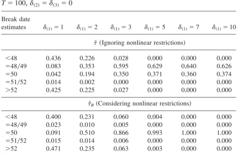
gration relations without presenting detailed results+The latter DGP has been considered to study the properties of the procedures in the case of more com- plicated processes+Finally, we examine situations whered₁⫽ ⫺Pd⫽0 and, hence,according to Theorems 3+1~i!and 3+2~i!,consistent estimation requires larger shift sizes+

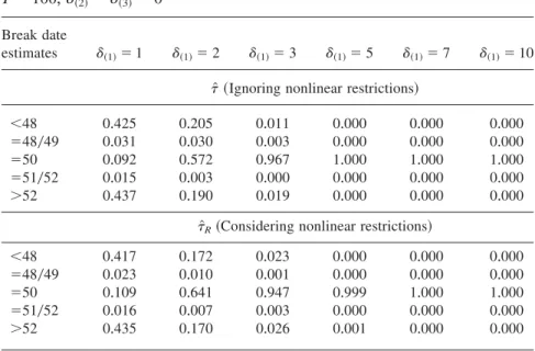
The break date estimates with respect to our three-dimensional basis DGP withr⫽1 and a VAR order p⫽1 are reported in Table 2 and Figure 1a+We consider a shiftd⫽~d~1!,d~2!,d~3!!^' with d~1! ranging from 1 to 10 and d~2!⫽ d~3!⫽0+Hence,the shift occurs in the first component of the DGP,which is stationary according to ~5+1!+Thus,as discussed before, we haved1⫽Pd⫽ ab^'d⫽0 in~3+1!and,hence,u⫽b^'d⫽0 in~2+7!+

The performance of the estimatorst[Randt[ is very similar,although the for- mer estimator is more successful in finding the correct break date for small shift magnitudes+Only ifd~1!⫽3 andd~1!⫽5 does t[ perform slightly better+

For large values ofd~1!both estimators perform identically+In fact,the cases of d~1!⫽3 andd~1!⫽5 represent the few exceptions in all our simulation experi- ments wheret[ outperformst[R+These observations also hold if one considers the small band @t ⫺ 2; t ⫹2# instead of the single true value of t only to evaluate the break date estimator+The frequency of break date estimatest[ and

[

tRin the interval@t⫺2;t⫹2#is denoted by t~band![ andt[R~band!,respec- tively,in Figure 1+Obviously,the frequency of finding the truetincreases for

Table2. Break date estimates for three-dimensional DGP with r⫽1 ~c1⫽ 0+9!,Q⫽~0+4, 0+8!,VAR order p⫽1,true break point t⫽ 50,sample size T⫽100,d_~2!⫽d_~3!⫽0

Break date

estimates d~1!⫽1 d~1!⫽2 d~1!⫽3 d~1!⫽5 d~1!⫽7 d~1!⫽10

[

t ~Ignoring nonlinear restrictions!

,48 0+425 0+205 0+011 0+000 0+000 0+000

⫽48049 0+031 0+030 0+003 0+000 0+000 0+000

⫽50 0+092 0+572 0+967 1+000 1+000 1+000

⫽51052 0+015 0+003 0+000 0+000 0+000 0+000

.52 0+437 0+190 0+019 0+000 0+000 0+000

[

tR~Considering nonlinear restrictions!

,48 0+417 0+172 0+023 0+000 0+000 0+000

⫽48049 0+023 0+010 0+001 0+000 0+000 0+000

⫽50 0+109 0+641 0+947 0+999 1+000 1+000

⫽51052 0+016 0+007 0+003 0+000 0+000 0+000

.52 0+435 0+170 0+026 0+001 0+000 0+000

larger shift magnitudes+This result is not surprising given the asymptotic prop- erties of the estimators and the fact thatd1⫽0 in the present situation+Because Tis fixed,changingd~1!from 1 to 10 may be interpreted as changingaord*in Assumption 3 accordingly+

Next, we have fitted a VAR~3! model although the true DGP has only an orderp⫽1,and we give the results in Table 3 and Figure 1b+In this casej0⫽0 in Theorem 3+1~i! because g1⫽ g2 ⫽ 0+ Thus, under the conditions of that theorem,Pr$48ⱕt[ ⱕ50%r1+In line with this result,t[ does not find the true break pointt⫽50 even ifd~1! is large+In fact,we observe in Table 3 that in about two-thirds of the replications the break date is located too early+How- ever,the estimates converge to the stated range fort,[ in line with our asymp- totic results+ Interestingly,focusing on the band @t⫺2;t ⫹2#,t[ is slightly more successful thant[_Rford_~1!⫽2 and 3~see Figure 1b!+

To analyze possible effects of the location oftwe also studied break points t⫽10, 25,75,and 90 using the same three-dimensional DGP as before+We found that it is only slightly more difficult to detect the more extreme break points if small shift magnitudes are considered+In the case of large shift mag- nitudes the location of the break date becomes even less important for the esti- mation results+These observations were made for both break date estimators and both VAR ordersp⫽1 and 3+

Next,we studied the effect of the error term correlation between the station- ary and nonstationary components by considering a three-dimensional DGP as before but withQ⫽~0,0!and comparing the outcomes with the previous find- ings+The absence of instantaneous error term correlation made it more difficult for both estimators to locate the true break point regardless of the lag order+

This outcome can be explained by the fact that we considered a shift only in one of the three components so that a weaker link of the components owing to Q⫽~0,0!complicated the break date search+In this situation,t[R was always Figure1. Relative frequency of true break point estimates~t,[ t[R! or of estimates in intervalt 62~t ~band!,[ t[R~band!!for three-dimensional DGP withr⫽1~c1⫽0+9!, Q⫽~0+4,0+8!,sample sizeT⫽100,true break pointt⫽50,d~2!⫽d~3!⫽0+

the most successful procedure, and usually its advantage was even more pro- nounced than in the case ofQ⫽~0+4,0+8!+

Our results with respect to the more complicated four-dimensional DGP with a cointegrating rankr⫽2 ~c₁⫽c₂⫽0+7! andQ⫽~ @0+4:0+4#^':@0+4:0+4#^'! clearly indicated that the performance of the break date estimators deteriorates in the case of smaller level shifts+ We chose a shift vector of the form d ⫽

~d_~1!,d_~2!,d_~3!,d_~4!!^'withd_~1!ranging again from 1 to 10 andd_~2!⫽d_~3!⫽d_~4!⫽0+

By adding a further dimension to the process the importance of the break in only one component is weakened,which may explain the lower number of cor- rect break date estimates+ The relative rankings of the two estimation proce- dures did not change,however+

Finally,we examined two DGPs for whichd1⫽Pd⫽0+For this situation, Theorems 3+1 and 3+2 state that compared to the case d1⫽ 0 “larger” shift magnitudes are needed to ensure thatt[ andt[Rcan estimate the break date con- sistently+First,we considered a three-dimensional process as in the base case but withd~3!ranging from 1 to 10 andd~1!⫽d~2!⫽0+Because the shift occurs in the third component,which is nonstationary,the level shift is orthogonal to the cointegration space in line with our DGP design~5+1!+Thus,we simulated a case of co-breaking+Second,we used a three-dimensional process withc1⫽1 so that the cointegrating rank isr⫽0+In the case ofr⫽0,all components of the DGP are nonstationary,and therefore no error term correlation is present becauseQvanishes+

Table3. Break date estimates for three-dimensional DGP with r⫽1 ~c₁⫽ 0+9!,Q⫽~0+4, 0+8!,VAR orderp⫽ 3, true break pointt ⫽50,sample size T⫽100,d_~2!⫽d_~3!⫽0

Break date

estimates d~1!⫽1 d~1!⫽2 d~1!⫽3 d~1!⫽5 d~1!⫽7 d~1!⫽10

[

t ~Ignoring nonlinear restrictions!

,48 0+436 0+226 0+028 0+000 0+000 0+000

⫽48049 0+083 0+353 0+595 0+629 0+640 0+626

⫽50 0+042 0+194 0+350 0+371 0+360 0+374

⫽51052 0+014 0+002 0+000 0+000 0+000 0+000

.52 0+425 0+225 0+027 0+000 0+000 0+000

[

tR~Considering nonlinear restrictions!

,48 0+400 0+231 0+060 0+004 0+000 0+000

⫽48049 0+023 0+010 0+005 0+000 0+000 0+000

⫽50 0+091 0+510 0+866 0+993 1+000 1+000

⫽51052 0+015 0+014 0+006 0+000 0+000 0+000

.52 0+471 0+235 0+063 0+003 0+000 0+000

The results for the shift date estimators are depicted in Figure 2+Clearly,it was more difficult for both procedures to locate t in this situation+ In par- ticular, the case of no cointegration is much more difficult to deal with than co-breaking ~compare Figures 2c and 2d with Figures 2a and 2b!+The poor performance of the shift date estimation procedures for small shift sizes rela- tive to DGPs with d₁⫽0 is in accordance with the finding in Section 3 that precise estimation requires large shift magnitudes ifd1⫽0+

To sum up,the constrained estimator t[R is usually at least as good ast[ and often superior in finding the true break date+The small-sample results fort[ are in line with our asymptotic derivations,which say that this procedure may esti- mate the break date too early when the VAR order is overspecified+

So far we have just analyzed the small-sample properties of the break date estimators in terms of their ability to locate the true shift date+If one is primar- ily interested in the cointegrating rank of the system the focus should be on the small-sample properties of the cointegration tests based on these different esti- mators+Our main conclusion is that the tests’ small-sample size and power dif- fer very little even in those cases where the break date estimators perform differently+Therefore,we only discuss the outcomes for our three-dimensional base DGP for which we haved1⫽Pd⫽0,the case treated in Theorem 4+1+

Figure2. Relative frequency of true break point estimates~t,[ t[R! or of estimates in intervalt 62~t ~band!,[ t[_R~band!!for three-dimensional DGPs withQ⫽~0+4,0+8! ~a and b!,Q⫽~0,0! ~c and d!,sample sizeT⫽100,true break pointt⫽50+