on Repeated Measures:
Gaussian Process Panel and Person-Specific EEG Modeling
Dissertation
zur Erlangung des akademischen Grades Doctor rerum naturalium
(Dr. rer. nat.)
eingereicht an der Lebenswissenschaftlichen Fakult¨ at der Humboldt-Universit¨ at zu Berlin
von Dipl.-Inform. Julian David Karch
Pr¨ asident der Humboldt-Universit¨ at zu Berlin:
Prof. Dr.-Ing. habil. Dr. Sabine Kunst Dekan der Lebenswissenschaftlichen Fakult¨ at:
Prof. Dr. rer. nat. Dr. Richard Lucius
Gutachter
1. Prof. Dr. Manuel C. Voelkle 2. Prof. Dr. Steven M. Boker 3. Prof. Dr. Thad Polk
Tag der m¨ undlichen Pr¨ ufung: 10.10.2016
Hiermit erkl¨are ich an Eides statt,
• dass ich die vorliegende Arbeit selbstst¨andig und ohne unerlaubte Hilfe verfasst habe,
• dass ich mich nicht bereits anderw¨arts um einen Doktorgrad beworben habe und keinen Doktorgrad in dem Promotionsfach Psychologie besitze,
• dass ich die zugrunde liegende Promotionsordnung vom 11. Februar 2015 kenne.
Berlin, den 28.06.2016
Julian D. Karch
This dissertation is the outcome of research that I conducted within the research project
“Formal Methods in Lifespan Psychology” at the Center for Lifespan Psychology of the Max Planck Institute for Human Development in Berlin. During my dissertation work, I also became affiliated with the “Psychological Research Methods” chair at the Hum- boldt University Berlin. Thus, many people have contributed to the success of this thesis.
Especially, I want to thank:
Andreas Brandmaier for his excellent mentoring throughout this thesis. In particu- lar, his constant availability for discussions has far exceeded what can be expected from a thesis advisor. To this day, I am still surprised how fast problems can be resolved when discussing them with him.
Manuel V¨olkle for his excellent co-mentoring of the thesis. He always gave important support and help.
Ulman Lindenberger, the director of the Center for Lifespan Psychology, for always being supportive of my work.
Markus Werkle-Bergner, Myriam Sander, and Timo von Oertzen for co-authoring the first paper that resulted as part of my dissertation work.
Timo von Oertzen also for convincing me in the first place that the Center for Lifespan Psychology is a great place to work, and for his continuing methodological advice.
Janne Adolf and Charles Driver, my fellow PhD students within the Formal Meth- ods project, for countless hours of helpful discussion.
Janne Adolf also for proofreading the introduction, the discussion, and Chapter 2, and for repeatedly suggesting valuable literature.
Steven Boker, Thad Polk, Matthias Ziegler, and Martin Hecht, my committee mem- bers, for being willing to invest time and effort in this thesis.
Julia Delius for providing highly valuable editorial assistance.
Florian Schmiedek for providing the COGITO data set.
The work presented in Chapter 5 has already been published:
Karch, J. D., Sander, M. C., von Oertzen, T., Brandmaier, A. M., & Werkle-Bergner, M.
(2015). Using within-subject pattern classification to understand lifespan age differences in oscillatory mechanisms of working memory selection and maintenance. NeuroImage, 118, 538–552. doi:10.1016/j.neuroimage.2015.04.038
Here, I embed this project within the remaining work of my dissertation, and focus on the methodological aspects. My contributions for the original publication were:
Programming: entirely; data analysis: entirely; compiling of the manuscript: largely;
development of methods: largely; reasoning: largely; literature research: largely; discus- sion of the results: predominantly; original idea: partially.
Wiederholte Messungen mehrerer Individuen sind von entscheidender Bedeutung f¨ur die entwicklungspsychologische Forschung. Nur solche Datenstrukturen erlauben die notwendige Trennung von Unterschieden innerhalb von und Unterschieden zwischen Per- sonen. Beispiele sind l¨angsschnittliche Paneldaten und Elektroenzephalografie-Daten (EEG-Daten). In dieser Arbeit entwickle ich f¨ur jede dieser beiden Datenarten neue Analyseans¨atze, denen Methoden des maschinellen Lernens zu Grunde liegen.
F¨ur Paneldaten entwickle ich Gauß-Prozess-Panelmodellierung (GPPM), die auf der flexiblen Bayesschen Methode der Gauß-Prozess-Regression basiert. Damit GPPM dem psychologischen Fachpublikum zug¨anglich wird, leite ich außerdem begleitende frequen- tistische Inferenzverfahren her. Der Vergleich von GPPM mit l¨angsschnittlicher Struk- turgleichungsmodellierung (SEM), welche die meisten herk¨ommlichen Panelmodellie- rungsmethoden als Sonderf¨alle enth¨alt, zeigt, dass l¨angsschnittliche SEM wiederum als Sonderfall von GPPM aufgefasst werden kann. Im Gegensatz zu l¨angsschnittlicher SEM eignet sich GPPM gut zur zeitkontinuierlichen Modellierung, kann eine gr¨oßere Menge von Modellen beschreiben, und beinhaltet einen einfachen Ansatz zur Generierung per- sonenspezifischer Vorhersagen. Wie ich ebenfalls zeige, stellt auch die zeitkontinuierliche Modellierungstechnik der Zustandsraummodellierung – trotz vieler Unterschiede – einen Spezialfall von GPPM dar. Ich demonstriere die Vielseitigkeit von GPPM anhand zweier Datens¨atze und nutze dazu die eigens entwickelte GPPM-Toolbox. F¨ur ausgew¨ahlte popul¨are l¨angsschnittliche Strukturgleichungsmodelle zeige ich, dass die implementierte GPPM-Darstellung gegen¨uber bestehender SEM Software eine bis zu neunfach beschle- unigte Parametersch¨atzung erlaubt.
F¨ur EEG-Daten entwickle ich einen personenspezifischen Modellierungsansatz zur Identifizierung und Quantifizierung von Unterschieden zwischen Personen, die in konven- tionellen EEG-Analyseverfahren ignoriert werden. Im Rahmen dieses Ansatzes wird aus einer großen Menge hypothetischer Kandidatenmodelle das beste Modell f¨ur jede Person ausgew¨ahlt. Zur Modellauswahl wird ein Verfahren aus dem Bereich des maschinellen Lernens genutzt. Als Kandidatenmodelle werden Vorhersagefunktionen verwendet, die die EEG-Daten mit Verhaltensdaten verbinden. Im Gegensatz zu klassischen Anwen- dungen maschinellen Lernens ist die Interpretation der ausgew¨ahlten Modelle hier von entscheidender Bedeutung. Aus diesem Grund zeige ich, wie diese sowohl auf der Personen- als auch auf der Gruppenebene interpretiert werden k¨onnen. Ich validiere den vorgeschlagenen Ansatz anhand von Daten zur Arbeitsged¨achtnisleistung. Die Ergebnisse verdeutlichen, dass die erhaltenen personenspezifischen Modelle eine genauere Beschreibung des Zusammenhangs von Verhalten und Hirnaktivit¨at erm¨oglichen als kon- ventionelle, nicht personenspezifische EEG-Analyseverfahren.
Repeated measures obtained from multiple individuals are of crucial importance for de- velopmental research. Only they allow the required disentangling of differences between and within persons. Examples of repeated measures obtained from multiple individuals include longitudinal panel and electroencephalography (EEG) data. In this thesis, I develop a novel analysis approach based on machine learning methods for each of these two data modalities.
For longitudinal panel data, I develop Gaussian process panel modeling (GPPM), which is based on the flexible Bayesian approach of Gaussian process regression. For GPPM to be accessible to a large audience, I also develop frequentist inference procedures for it. The comparison of GPPM with longitudinal structural equation modeling (SEM), which contains most conventional panel modeling approaches as special cases, reveals that GPPM in turn encompasses longitudinal SEM as a special case. In contrast to longi- tudinal SEM, GPPM is well suited for continuous-time modeling, can express a larger set of models, and includes a straightforward approach to obtain person-specific predictions.
The comparison of GPPM with the continuous-time modeling technique multiple-subject state-space modeling (SSM) reveals, despite many differences, that GPPM also encom- passes multiple-subject SSM as a special case. I demonstrate the versatility of GPPM based on two data sets. The comparison between the developed GPPM toolbox and existing SEM software reveals that the GPPM representation of popular longitudinal SEMs decreases the amount of time needed for parameter estimation up to ninefold.
For EEG data, I develop an approach to derive person-specific models for the iden- tification and quantification of between-person differences in EEG responses that are ignored by conventional EEG analysis methods. The approach relies on a framework that selects the best model for each person based on a large set of hypothesized candidate models using a model selection approach from machine learning. Prediction functions linking the EEG data to behavior are employed as candidate models. In contrast to classical machine learning applications, interpretation of the selected models is crucial.
To this end, I show how the obtained models can be interpreted on the individual as well as on the group level. I validate the proposed approach on a working memory data set. The results demonstrate that the obtained person-specific models provide a more accurate description of the link between behavior and EEG data than the conventional nonspecific EEG analysis approach.
Eidesstattliche Erkl¨arung i
Acknowledgements ii
Contributions iii
Zusammenfassung iv
Abstract v
Acronyms ix
1. Introduction 1
1.1. Gaussian Process Panel Modeling . . . 1
1.2. Person-Specific EEG Modeling . . . 3
1.3. Outline . . . 6
2. Statistical Inference and Supervised Machine Learning 7 2.1. Foundations of Statistical Inference . . . 7
2.2. Statistical Inference as a Decision Problem . . . 11
2.3. Frequentist Inference . . . 13
2.3.1. Foundations . . . 13
2.3.2. Point Estimation . . . 15
2.3.3. Set Estimation . . . 16
2.3.4. Hypothesis Testing . . . 17
2.4. Bayesian Inference . . . 20
2.4.1. Point Estimation . . . 21
2.4.2. Set Estimation . . . 21
2.4.3. Hypothesis Testing . . . 22
2.5. Supervised Machine Learning . . . 22
2.6. Connections Between Supervised Learning and Statistical Inference . . . . 24
2.7. Model Validation and Model Selection . . . 25
2.7.1. Model Validation . . . 25
2.7.2. Model Selection . . . 26
3. Gaussian Process Panel Modeling 27 3.1. General Linear Model . . . 28
3.2. Structural Equation Modeling . . . 29
3.2.1. Structural Equation Models . . . 30
3.2.2. Frequentist Inference . . . 32
3.2.3. Model Validation and Selection . . . 35
3.2.4. Longitudinal Structural Equation Modeling . . . 36
3.3. Gaussian Process Regression . . . 38
3.3.1. Weight-Space View . . . 38
3.3.2. Function-Space View . . . 40
3.3.3. Model Selection . . . 42
3.3.4. Model Validation . . . 45
3.4. Gaussian Process Time Series Modeling . . . 45
3.4.1. Foundations . . . 45
3.4.2. Extension to Multivariate Time Series . . . 47
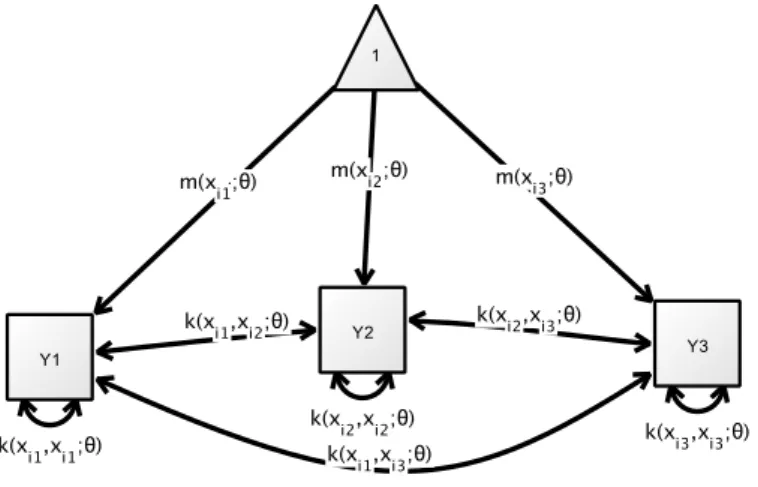
3.5. Gaussian Process Panel Models . . . 49
3.5.1. Foundations . . . 49
3.5.2. Model Specification . . . 50
3.6. Inter-Individual Variation in Gaussian Process Panel Models . . . 51
3.6.1. Observed Heterogeneity . . . 51
3.6.2. Introduction to Unobserved Heterogeneity . . . 53
3.6.3. Implementation of Unobserved Heterogeneity . . . 54
3.6.4. Mixing Observed and Unobserved Heterogeneity . . . 55
3.6.5. Limitations for Unobserved Heterogeneity . . . 55
3.7. Statistical Inference for Gaussian Process Panel Models . . . 57
3.7.1. Point Estimation . . . 58
3.7.2. Hypothesis Testing . . . 58
3.7.3. Confidence Regions . . . 59
3.7.4. Person-Specific Prediction . . . 59
3.7.5. Model Selection and Validation . . . 60
3.8. Implementation of Gaussian Process Panel Modeling . . . 62
3.8.1. Model Specification . . . 62
3.8.2. Maximum Likelihood Estimation . . . 62
3.8.3. Hypothesis Testing . . . 64
3.9. Related Work . . . 65
4. Advantages of Gaussian Process Panel Modeling 67 4.1. Relationships to Conventional Longitudinal Panel Modeling Approaches . 67 4.1.1. Longitudinal Structural Equation Modeling . . . 67
4.1.2. State-Space Modeling . . . 75
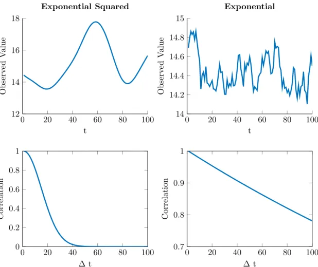
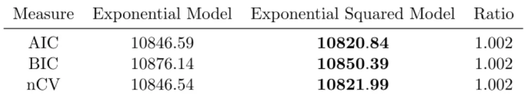
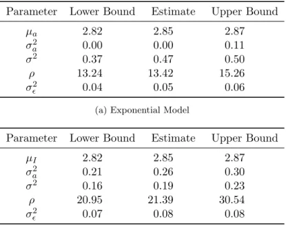
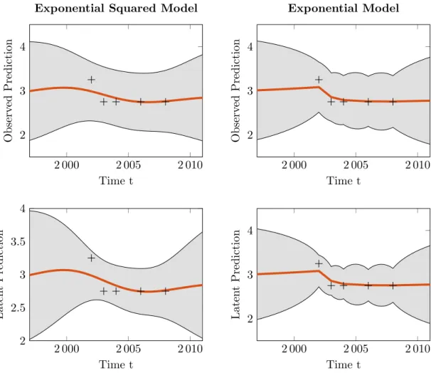
4.2. Demonstration of Gaussian Process Panel Modeling . . . 80
4.2.1. Exponential Squared Covariance Function as Alternative to the Autogressive Model . . . 80
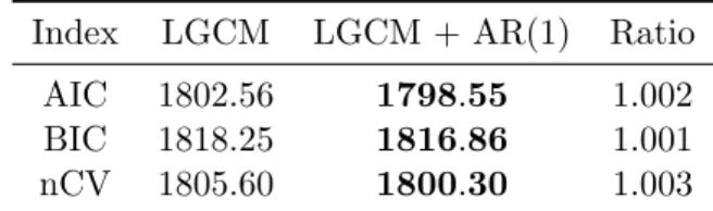
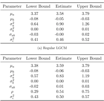
4.2.2. Extending LGCMs With Autocorrelated Error Structures . . . 88
4.3. Fitting Speed Comparison of Gaussian Process Panel Modeling and Struc-
tural Equation Modeling Software . . . 96
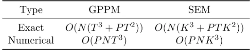
4.3.1. Theoretical Comparison . . . 96
4.3.2. Empirical Comparison . . . 103
5. Person-Specific EEG Modeling Based on Supervised Learning 110 5.1. Identifying Person-Specific Models: The Supervised Learning Approach . 111 5.1.1. Foundations . . . 111
5.1.2. Candidate Models . . . 114
5.1.3. Spatial Interpretation of the Best Estimated Model . . . 116
5.2. Working Memory Data Set and Preprocessing . . . 120
5.2.1. Study Design . . . 120
5.2.2. Preprocessing . . . 121
5.2.3. Data Analysis . . . 122
5.3. Results . . . 122
5.3.1. Performance Evaluation Against Chance and the Best Nonspecific Model . . . 122
5.3.2. Person-Specific Results . . . 125
5.3.3. Group Results . . . 128
5.3.4. Performance Comparison Against Simpler Person-Specific Models . 132 6. Summary and Discussion 136 6.1. Gaussian Process Panel Modeling . . . 136
6.2. Person-Specific EEG Modeling . . . 140
6.3. Conclusion . . . 142
References 143 A. Probability Theory 154 A.1. Foundations of Probability Theory . . . 154
A.2. Conditional Distributions and Independence . . . 156
A.3. (Co)Variance Rules and the Gaussian Distribution . . . 158
B. Person-Specific Results 162 B.1. Attentional Focus . . . 163
B.2. Working Memory Load . . . 168
AIC Akaike information criterion ANOVA analysis of variance AR autoregressive
BAC balanced accuracy BCI brain–computer interface BIC Bayesian information criterion CI confidence interval
CSP common spatial pattern DV dependent variable EEG electroencephalography ERP event-related potential GLM general linear model GP Gaussian process
GPML Gaussian processes for machine learning GPR Gaussian process regression
GPPM Gaussian process panel modeling/model GPTSM Gaussian process time series modeling/model HLM hierarchical linear modeling/model
ICA independent component analysis iff if, and only if,
iid independent and identically distributed IV independent variable
LGCM latent growth curve model MAP maximum a posteriori MLR multiple linear regression ML maximum likelihood
MRI magnetic resonance imaging LDA linear discriminant analysis
LLDA Ledoit’s linear discriminant analysis PCA principal component analysis
pdf probability density function RAM reticular action model
SDE stochastic differential equation SEM structural equation modeling/model SSM state-space modeling/model
WM working memory
Repeated measures obtained from multiple individuals potentially on multiple variables are of crucial importance for developmental research. Only such data allow implementa- tion of the corresponding rationales put forward by Baltes and Nesselroade (1979). These encompass: the “direct identification of intra-individual change [and variation]” (Baltes
& Nesselroade, 1979, p. 23), the “direct identification of inter-individual differences”
therein (Baltes & Nesselroade, 1979, p. 24), and the “analysis of interrelationships of . . . change” (Baltes & Nesselroade, 1979, p. 26). To analyze such data, a model for inter-individual as well as intra-individual variation is required. In this thesis, I adopt a machine learning perspective on modeling repeated measures data. Besides recontex- tualizing traditional inference methods for model selection and validation, this mainly involves proposing two novel modeling approaches, each tailored to a specific instance of multiple individuals’ repeated measures data. For longitudinal panel data, I propose Gaussian process panel modeling (GPPM), and for EEG data, I propose a method to de- rive person-specific models. Both approaches extend conventional modeling approaches.
Specifically, they are not subject to assumptions rarely met for psychological phenomena and thus model multiple individuals’ repeated measures data more appropriately.
1.1. Gaussian Process Panel Modeling
For longitudinal panel studies (referred to as panel studies in the following), the most widely used method for formulating a model of intra-individual variation is the general linear model (GLM) with chronological time asindependent variable (IV) and the char- acteristic of interest as dependent variable (DV). Often, other than time, further IVs that are hypothesized to explain both intra-individual and inter-individual variation are included. To allow for inter-individual variation that is not explained by the IVs, the GLM is typically extended to the hierarchical linear model (HLM), in which, in con- trast to the GLM, the mapping from the IVs to the DV can vary between persons. A prominent example of a HLM for panel data is the latent growth curve model (LGCM) in which linear growth rates are assumed to vary between persons.
Structural equation modeling (SEM) is a modeling technique that generalizes all linear, multivariate statistical models such as the t-test, paired t-test, or analysis of variance (ANOVA) (Fan, 1997; Knapp, 1978). It can be shown that the HLM is also a special case of SEM (Curran, 2003). SEM is widely used to model panel data. In this thesis,longitudinal SEM will refer to using SEM for panel data.
Model specification in SEM consists of formulating a set of linear equations that describe the hypothesized relationships between a set of variables. Accordingly, it suffers
from two major limitations: First, only linear relationships between variables can be modeled, and second, the number of variables is necessarily finite. The second limitation is especially problematic for panel data. It leads to the problem that longitudinal SEM only allows expression of discrete-time models. Thus, longitudinal SEM does not permit to model development over time as what it is, namely a continuous-time process. To model continuous-time processes, it is necessary to employ continuous-time modeling.
Besides this conceptual advantage, continuous-time modeling also has the advantage that it does not rely on assumptions that can seldom be met in practice. Using discrete- time models, it is assumed that all measurements have been taken at the same time points for all individuals, and that the interval between any two successive measurements is the same. This assumption is rarely met in actual panel studies, in which an occasion of measurement needs to be spread over weeks or months, typically due to limited testing facilities.
One remedy to the problem of longitudinal SEM only being able to express discrete- time models is to use an underlying continuous-time model and generate the correspond- ing discrete-time structural equation model (SEM) for a given data set. For LGCM this can be straightforwardly achieved. Voelkle, Oud, Davidov, and Schmidt (2012) use this approach to derive a SEM representation of the continuous-time autoregressive (AR) model. However, their solution relies on extensions of the conventional SEM approach.
The resulting modeling technique is known as extended SEM (Neale et al., 2016), which captures a broader scope of models. This solution is in the spirit of fitting available tools to new problems.
In this thesis, I propose a different approach. Instead of using SEM or extensions of it, I suggest that a more suitable technique that is able to represent continuous-time models directly should be employed. To this end, I systematically introduce the continuous-time time series modeling technique Gaussian process time series modeling (GPTSM) as a novel tool for statistical modeling of psychological time series data.
GPTSM is based on Gaussian process regression (GPR), which is a flexible function- fitting approach. GPR has recently gained popularity in the field of machine learning as a Bayesian nonparametric regression technique. GPTSM has already been used in fields such as machine learning (Cunningham, Ghahramani, & Rasmussen, 2012; Saat¸ci, Turner, & Rasmussen, 2010) and physics (Roberts et al., 2013). Within psychology, I am only aware of two applications of GPTSM (Cox, Kachergis, & Shiffrin, 2012;
Ziegler, Ridgway, Dahnke, & Gaser, 2014). Both applications adapt GPTSM for specific problems rather than introducing and discussing the method for psychological research in a broader context.
I extend the time series method GPTSM for use on panel data. A panel data set can be interpreted as consisting of a time series for each person. Thus, to extend the time series method GPTSM to panel data, a mechanism allowing formulation of a simultaneous model for multiple time series needed to be composed. I develop one straightforward and unified approach, and call the resulting model familyGaussian process panel models (GPPMs). In principle, the Bayesian inference methods used for Gaussian process time series models (GPTSMs) could also be used for GPPMs. However, within psychology
frequentist inference is still the de-facto standard approach. Thus, for the method to be interpretable within common statistical reference frames and to be accessible to a large audience, I also develop frequentist inference procedures for GPPMs, and call the resulting methodGaussian process panel modeling (GPPM).
While an extension of GPTSM for panel data has already been discussed briefly within the field of statistics (Hall, M¨uller, & Yao, 2008), a full presentation of a panel modeling approach based on GPTSM, with a full set of corresponding inference procedures and a detailed comparison with conventional panel methods, as I perform here, is still lacking.
Also, GPPM is substantially different then the approach proposed by Hall et al. (2008).
One main difference is that I propose using parametric estimators, whereas Hall et al.
(2008) propose applying nonparametric estimators. To the best of my knowledge, my work is the first work to discuss the extension of GPTSM for modeling of psychological panel data.
Besides GPTSM, other continuous-time modeling techniques could have been used as a basis for a panel modeling framework. Indeed, Oud and Singer (2008), Boker (2007a) have extended the continuous-time time series method state-space modeling (SSM) for panel data (i.e., for multiple subjects). I will come back to the difference between multiple-subject SSM and GPPM later.
In this thesis, I examine the properties of GPPM in detail. Specifically, I compare GPPM against longitudinal SEM and multiple-subject SSM. Interestingly, this compar- ison reveals that both longitudinal SEM and multiple-subject SSM can be regarded as special cases of GPPM. At the same time, GPPM extends both methods. I provide examples of models that can only be expressed using GPPM, and show that they are vi- able alternatives to related models that are typically used in psychological research. One interesting difference between the continuous-time modeling methods multiple-subject SSM and GPPM is that in GPPM the to-be-modeled process is described explicitly as a function of the IVs, whereas in multiple-subject SSM the process is described implicitly via the dynamics of the process.
In this thesis, I also examine whether expressing longitudinal models as GPPM and using GPPM software to estimate parameters is faster then using the equivalent longi- tudinal SEM. My findings suggest that GPPM software is indeed faster, and, thus, the use of GPPM software for conventional SEM may either allow the use of larger-scale models or a significant increase of fitting speed.
1.2. Person-Specific EEG Modeling
Since GPPM is a parametrical method, it is well suited as a data-analytic approach for situations in which a parametric model for intra-individual and inter-individual variation is available, for example, based on theory or previous empirical work. However, in many situations such a model might not be readily available. A typical example are brain imaging data such as EEG data. In this case, the conventional analysis approach treats both the intra-individual and the inter-individual variation as measurement error. In the second part of this thesis, I propose a new analysis strategy based on techniques
from the field of machine learning to account for inter-individual variation in EEG data sets by adopting a person-specific analysis approach (e.g., Molenaar & Campbell, 2009).
The approach is general enough that it could also be applied to other brain-imaging methods such as magnetic resonance imaging (MRI).
In EEG studies, researchers are typically interested in estimating event-related poten- tials (ERPs). An ERP is the measured brain response caused by a given behavior, such as looking at a certain stimulus. To estimate person-specific ERPs, the behavior of in- terest is repeated multiple times for each person. The repetitions are commonly referred to as trials. The person-specific ERPs are obtained by averaging across all repetitions for each person. Thus, intra-individual variation in the the brain–behavior mapping is considered as measurement error.
To compare ERPs evoked by a given behavior between groups like younger and older adults, conventional statistical procedures like thet-test or ANOVA are commonly em- ployed. Certain features of interest of the person-specific ERPs are used as the DV, e.g., the mean amplitude in a given time window. Group membership is the IV. Thus, while this approach specifically focuses on variation between groups, the inter-individual variation within each group is treated as measurement error. Consequently, conventional ERP analysis treats both inter-individual and intra-individual variation as measurement error. Accordingly, in order for the group-average ERPs to be representative of the true brain response for a given person at a given time point, both the intra-individual and inter-individual variation have to be sufficiently low. Empirical data suggests that at least the assumption of small inter-individual variation is not met for children and older adults, since an increased heterogeneity of functioning in behavioral tasks is observed (e.g., Astle & Scerif, 2011; Nagel et al., 2009; Werkle-Bergner, Freunberger, Sander, Lindenberger, & Klimesch, 2012).
One solution to account for the observed inter-individual variation is to adopt a person- specific analysis strategy as propagated, for example, by Molenaar (2013). Using the conventional ERP analysis approach, this could in principle be achieved by performing a separate statistical analysis for each person. However, the signal-to-noise ratio in EEG data is typically not high enough to make this approach feasible in practice. The statistical power of this approach would be too low for most available EEG data sets.
Even worse, since the very idea of performing the analysis on the person-specific level means allowing the link between behavior and EEG signal to vary between persons, many statistical tests would have to be performed, one for each hypothesized univariate link between behavior and brain (i.e., for each feature of the EEG like the mean amplitude within a given channel and time window), decreasing statistical power even further.
To solve the problems of a low signal-to-noise ratio and low statistical power, I propose adapting techniques from the field ofbrain–computer interface (BCI) research (Wolpaw
& Wolpaw, 2012). Here, the goal is to predict a participants’ brain state given the data of only a single trial. Thus, one may see this data analysis method as a reversal of the conventional ERP approach. Instead of finding a mapping from a behavior to one feature of an ERP, and repeating this process for different features (a so-called mass univariate approach), one tries to find a mapping from the complete EEG signal
of one trial to the behavior (multivariate approach). In the MRI literature the former approach is known asencoding (from behavior to data) and the latter asdecoding (from data to behavior). Another name for the decoding approach within the MRI community is multi-voxel pattern analysis (MVPA). Aggregating over time and space solves the two main problems of person-specific ERP analysis, as previously identified. First, the signal-to-noise ratio can be increased by aggregating. Second, only one statistical test has to be performed per person.
In conventional BCI studies the ultimate goal is to enable people to control a device just with their thoughts, more precisely through specific, reliable activity patterns of their brains. To evaluate the utility of such an approach, the accuracy of the estimated brain–behavior mapping is of interest. In this study, however, interpreting individual brain–behavior mapping as person-specific model is of primary interest. The techniques employed within BCI research as well as in this work stem from the field of machine learning. In that field, mappings from IVs to the DV are typically found by using algorithms that select the best mapping based on a set of candidate mappings and a data set. Rather than a theory-driven confirmatory approach, the BCI approach may be seen as exploratory and entails selection between a large set of competing hypotheses that are data-driven. In BCI, an interpretation of the selected mapping is not of interest, and arbitrary complex mappings can be used as candidate mappings as a result. In contrast, the space of candidate mappings needed to be carefully restricted to be interpretable but still powerful enough to achieve a satisfying accuracy in this work. A complex, neural network regression approach, for example might be powerful but not interpretable.
A simple threshold model on a particular feature of the EEG signal (e.g., the mean amplitude within a given fixed time windows and channel) on the other hand might be interpretable but not powerful enough. To this end, I use a set of candidate models based on common spatial pattern (CSP) and linear discriminant analysis (LDA), which is commonly used for creating BCIs based on rhythmic neural activity (e.g., Blankertz et al., 2010; Fazli et al., 2009), and show how the resulting mapping can be meaningfully interpreted as person-specific models. In a second step, I demonstrate how the inter- individual variation of the found person-specific mappings can be explored as a proxy for the inter-individual variation of the true brain–behavior mapping.
To test the feasibility and utility of my approach, I re-analyzed data from a study that targeted brain oscillatory mechanisms for working memory (WM) selection and maintenance in a sample including children, younger, and older adults (Sander, Werkle- Bergner, & Lindenberger, 2012). We (Karch, Sander, von Oertzen, Brandmaier, &
Werkle-Bergner, 2015) selected this data set because we expected true inter-individual variation in the brain–behavior mapping, particularly in the older adults. Mixed results on the link between EEG and behavior exist with regard to the mechanism of WM.
Specifically, Sander et al. (2012) found evidence for attentional effects on the modulation of alpha power, whereas Vaden, Hutcheson, McCollum, Kentros, and Visscher (2012) did not observe any attention-related modulation in older adults. One explanation for the mixed results may be the increased inter-individual variation in older adults as compared to younger adults, which is ignored when using conventional analysis approaches but not
when applying the new analysis approach suggested here.
The results of using the proposed person-specific method to analyze the WM data set show that my approach leads to more accurate models than does the conventional analysis approach ignoring inter-individual variation. Thus, I challenge the implicit assumption that the observed inter-individual variation is measurement error. Interest- ingly, some aspects of the within-group inter-individual variation, as obtained by the proposed person-specific analysis strategy, was lower in older than in younger adults, which is contrary to what we (Karch et al., 2015) expected.
Thus, in this thesis, I present two new methods for the analysis of psychological data based on machine learning methods. The first, GPPM, is a new analysis method for panel data that both generalizes and extends conventional panel methods such as longitudinal SEM. The second method is a new analysis method for EEG data in which multivariate models are first estimated on the person level and then aggregated on the group level, explicitly addressing the within-group inter-individual variability, which is ignored by conventional analysis approaches.
1.3. Outline
In Chapter 2, I will start with a recapitulation of basic modeling principles that are necessary to understand the methods I will introduce later. The psychological curriculum rarely goes beyond frequentist statistics, which I will repeat nevertheless for the sake of completeness. Bayesian statistics and machine learning principles for modeling are usually left out. I will explain all three approaches from a single, unified perspective.
Before presenting the new longitudinal panel modeling method GPPM in chapter Chapter 3, I will introduce the techniques it is based on, the flexible Bayesian regression method GPR, and the time series analysis method GPTSM, which in turn is based on GPR. Because GPPM is later compared to the classical panel modeling method longitudinal SEM, and SEM was used as a source of inspiration for the development of GPPM, I also introduce SEM and, in particular, longitudinal SEM in Chapter 3.
I will discuss the advantages of GPPM over conventional panel methods, in particular longitudinal SEM and multiple-subject SSM, in Chapter 4, both theoretically and by providing examples. The examples also serve as a demonstration of GPPM. In this chapter, I furthermore compare the fitting speed of SEM and GPPM software, theoreti- cally and empirically. This was done to investigate whether formulating models in their GPPM representation may speed up parameter estimation as compared to the SEM representation.
In Chapter 5, I will present the person-specific EEG analysis in which first person- specific models are obtained and then second these person-specific models are summa- rized on the group level. I will also present the validation of the method based on data from the study targeting brain oscillatory mechanisms for WM selection and mainte- nance.
In Chapter 6, I summarize and discuss the results and contributions of my thesis as well as future research directions.
Machine Learning
Statistical inference revolves around making probabilistic statements about the proper- ties of a population based on a random, observed subset of the population. In psychology, an example for a property is the average general intelligence factorgof a given group, for example, older adults. The dominating approach to statistical inference in psychology is frequentist inference.
Supervised machine learning (abbreviated as supervised learning in the remainder) on the other hand, focuses on obtaining a prediction function on the base of a random, observed subset of the population. This function should predict a variable reliably based on some other variables for the complete population. Both statistical inference and supervised learning use a finite data set to obtain knowledge that should generalize to the population.
The popularity of Bayesian inference, in particular, (Lee & Wagenmakers, 2005; Wa- genmakers, Wetzels, Borsboom, & van der Maas, 2011) but also of supervised learning (Markowetz, Blaszkiewicz, Montag, Switala, & Schlaepfer, 2014; Yarkoni, 2012) is grow- ing within psychology. However, both are still not part of many psychological curricula.
This chapter, thus, serves the purpose of introducing Bayesian inference and supervised learning as alternative methods for modeling empirical data and making inferences from random samples. Before introducing Bayesian inference, it seems useful to reintroduce frequentist inference in a more formal manner than typically done in psychology teach- ing. This paves the way for the presentation of frequentist inference, Bayesian inference, and supervised learning within a single, coherent framework.
I will start this chapter by introducing the foundations of statistical inference in Sec- tions 2.1 and 2.2. A section explaining the frequentist and the Bayesian variants of statistical inference will follow. Then, I will introduce supervised learning and its connec- tion to statistical inference. In the final section, I will compare the different approaches (Bayesian, frequentist, and supervised learning) to model selection.
2.1. Foundations of Statistical Inference
A huge number of good textbooks introduce probability theory (e.g., DeGroot & Schervish, 2011; Rice, 2007; Taboga, 2012b; Wasserman, 2004). Thus, I provide only a swift re- minder to refamiliarize readers with probability theory in Appendix A. As the probability theory terminology differs slightly between authors, Appendix A also serves to present the terminology as used in this work.
The statistical literature aimed at psychologists typically introduces the topic of statis- tical inference in a rather informal manner (compare, for example, the current standard statistics book for psychologists in Germany [Eid, Gollwitzer, & Schmitt, 2013] with any general statistics text book [e.g., Wasserman, 2004]). This level does not suffice to understand the following chapters. Literature aimed at mathematicians or statisti- cians, however, requires more background knowledge than even the typical quantitative psychologist has learnt. Thus, I have tried to make this chapter as rigorous as possible without using advanced mathematical concepts (e.g., measurement theory and Borel sets) but limit myself to high school-level mathematics, that is, a good understanding of set theory, linear algebra, and calculus. I also assume that the reader has had first contact with frequentist inference.
The central task of statistical inference is to make probabilistic statements about the properties of a population based on a sample. Formally, a sample is defined as follows.
Definition 2.1.1. A sample y is a realization of a random vector Y.
Remark 2.1.2. A random vector is the generalization of a random variable. It is simply a vector that contains multiple random variables as entries. For a formal definition see Equation A.1.3 in Appendix A.1.
Example 2.1.3. For a longitudinal study during which 3 properties of 100 persons have been measured at 10 different time points the 3×100×10 data cube is a sample.
Thus, the task of making probabilistic statements about the population is formalized as making statements about the distribution that generated the sample. For now, I will describe this distribution via its distribution functionFY∗ and call it thetrue (generating) distribution in the following.
The statistical model is a central concept of statistical inference. It encodes the as- sumptions about the true distribution FY∗ before having observed the sample y. The assumptions are described by a set of candidate probability distributions forFY∗. Thus, a statistical model is merely a (typically infinite) set of probability distributions. For example, a statistical model is that the generating distribution FY∗ is a Gaussian distri- bution. Formally, a statistical model can be described as follows.
Definition 2.1.4. Let y be a sample with the corresponding n-dimensional random vectorY. LetB be the set of alln-dimensional distribution functions:
B :={F :Rn→R+such that F is a distribution function}
A subset M ⊂B is called a statistical model for Y. Remark 2.1.5. As notation, I will often use
Y ∼ M,
which reads that the statistical model for the random vector Y isM, or in other words that the random vector is distributed according to one of the distributions withinM.
If the assumptions about the generating distribution FY∗ are wrong, the statistical model is said to be misspecified; otherwise it is correctly specified.
Definition 2.1.6. LetFY∗ be the true generating distribution function andMa corre- sponding statistical model. IfFY∗ ∈ M, then the statistical model is said to becorrectly specified; otherwise it is misspecified.
In other words: the true generating distribution FY∗ has to be one of the probability distributions that constitute the statistical model.
Model specification is a crucial part of statistical inference. It refers to the process of developing a statistical model for an unknown distribution FY∗. It is important to realize that all traditional statistical inference procedures rely on the assumption that the statistical model is correctly specified. Otherwise, inference is formally invalid and to an unknown extent wrong.
In general, a statistical model M can be indexed by a possibly infinite dimensional index set Θ such that
M={Fθ :θ∈Θ}.
In the following, I will refer to this index set Θ as theparameter spaceand to its elements θ ∈Θ as parameter values. If a statistical model is correctly specified, a parameter θ∗ exists such that Fθ∗ = FY∗. Thus, in accordance with the literature, I will denote the generating distributionFY∗ by θ∗.
This work is only concerned with statistical models for continuous random vectors Y, for which the statistical model can equivalently be expressed in terms of a set of probability density functions (pdfs)instead of a set of distribution functions. Therefore, in the remainder, statistical models will be described as a set of pdfs:
M={pθ(y) :θ∈Θ}.
In psychology, a sample y is typically a sample from a population of persons. That is, the sample has the form y= [y1, . . . , yN]⊤, whereN refers to the number of persons.
Everyyi refers to the observed data for one person. The corresponding random vector Yi, of whichyi is a realization, contains the variables of interest, for example, the general intelligence factorg and socioeconomic status for a cross-sectional data set or repeated measurements of general intelligence factorg and socioeconomic status for a panel data set.
Typically, the assumption is made that the observationsyi for the different persons do not influence each other, for example, if it is known that the general intelligence factorg for person 7 is 110, this will not alter the expectation regarding the general intelligence factor of any other (unrelated) person. Formally, this is represented by the assumption that the random vectors{Yi :i∈1, . . . , N}are mutually independent.
Another assumption that is commonly made is that the observed data yi for each person are a realization of the same probability distribution. That is, the random vec- tors {Yi : i ∈ 1, . . . , N} are not only independent; every random vector is distributed according to the same distribution. Taken together, these two assumptions are known as theindependent and identically distributed (iid) assumption.
Definition 2.1.7. A set of random vectors {Yi : i ∈ 1, . . . , N} is independent and identically distributed (iid) if, and only if, (iff) each random vector Yi has the same probability distribution and if the random vectors are mutually independent.
If the iid assumption is made, the statistical model for the random vector Y can be determined by specifying a statistical model for the random vectors Yi. Because the random vectors are identically distributed, it is reasonable to use the same statistical model for each random vector Yi. The statistical model for the sample follows from the mutual independence assumption. Formally, if for all i∈ {1, . . . , N} the statistical model for each random vector Yi is
Yi∼ {pθ(yi) :θ∈Θ}, it follows that
Y ∼ {N
∏
i=1
pθ(yi) :θ∈Θ }
.
The two most common types of inference are estimation and hypothesis testing. In estimation, the aim is to eliminate some of the members of the statistical model as candidates for the true probability distributionθ∗. That is, in estimation, a restriction, which is formalized via a subset ΘR⊂Θ of the parameter space Θ, is selected such that a desirable property is fulfilled. For point estimation, the desired restriction implies a single point, that is,|ΘR|= 1. In point estimation it is common to denote the subset that implements the restriction via ˆθ∈Θ. In psychology, the most common point estimation technique ismaximum likelihood (ML) estimation.
Example 2.1.8. LetY consist ofN iid random vectorsYi and the statistical model for the random vectorsYi beYi ∼ {N(µ,1) :µ∈R}, then the ML estimate ˆµfor the mean µbased on a sample y= [y1, . . . , yN]⊤ is
ˆ µ= 1
N
∑N i=1
yi.
If the restriction ΘRcan contain more than one point, that is|ΘR|>1, one speaks of set estimation. Confidence intervals are a popular example for set estimation.
Example 2.1.9. Let the situation be set up as in Example 2.1.8, then a 95% confidence interval for the meanµis
[ˆµ−1.96,µˆ+ 1.96].
Hypothesis testing is strongly linked to set estimation. A restriction ΘR ⊂ Θ is proposed and either rejected or not.
Example 2.1.10. Let the situation be set up as in Example 2.1.8. A hypothesis test that rejects the restrictionµ= 0 if |ˆµ|>1.96 has the sizeα = 0.05.
Frequentist and Bayesian inference provide all these central inference types but achieve them in quite a different manner. I will try to convey the differences in the following.
However, I will first present the endeavor of statistical inference as a decision problem.
This will provide the formal basis to delineate the difference between the Bayesian and the frequentist approaches.
I will use the following notation without explicitly repeating it in all subsequent theo- rems and definitions. Y is the random vector for which a statistical modelM={pθ(y) : θ∈Θ}is proposed, y denotes one realization of Y, i.e., a sample, ΩY is the support of the random vector Y, that is, the set of all possible values that the realizations y can obtain, i.e.,y∈ΩY.
2.2. Statistical Inference as a Decision Problem
All types of statistical inference can be interpreted as decision problems. Given a sample y, a decision to (a) reject a hypothesis or not, (b) for a set of likely parameters ΘR⊂Θ, or (c) for a point estimate ˆθ ∈ Θ has to be made. With decision rules and actions, statistical decision theory provides the necessary tools for a unifying treatment of these different types of statistical inference. For hypothesis testing, for example, the decision rule is a hypothesis test and the action is to either reject the hypothesis or not. More generally, a decision rule is defined as follows.
Definition 2.2.1. A (deterministic) decision rule is a function δ: ΩY →A that maps every sample y ∈ Ωy onto an action δ(y) = a ∈ A (Berger, 1993, p. 9). The set of actionsA can be any non-empty set.
Remark 2.2.2. For point estimation, the decision rule is an estimator (often denoted θ(y)) that maps every data set to one particular parameter ˆˆ θ; typically called an estimate.
Thus, in this case the set of possible actions is the parameter space, A = Θ. For set estimation, the set of possible actionsA is the set of all possible subsets of the parameter space, called power set and denoted 2Θ. A set estimator maps every data set onto one member of the power set. For hypothesis testing, the set of possible actions is to either reject the proposed restriction ΘR⊂Θ of the parameter space or not. A hypothesis test maps every sample y to the decision to either reject a proposed restriction or not.
To evaluate a decision rule, its actions need to be evaluated. Each action is given a cost that depends on the true state of nature, i.e., the true generating probability distributionFY∗ ofY. For the moment I ignore the fact that the true distributionFY∗ is not known. The true distribution is assumed to be a member of the statistical model. As a consequence, the true distribution can be described by the parameterθ∗. By choosing a loss function, one can quantify how good an action is under the reality that is described by the true distribution θ∗.
Definition2.2.3. LetA be a set of possible actions of a decision functionδ: ΩY →A, then any non-negative function Ldefined on Θ×A is a loss function.
Example 2.2.4. For point estimation, the set of possible actionsA corresponds to the parameter space. Thus, for point estimation the loss function is a function that maps the true parameterθ∗ and a point estimate ˆθto a cost. One example for a loss function used for point estimation is the squared loss: Lsq(θ∗,θ) = (θˆ ∗−θ)ˆ2.
Remember that the loss function was introduced to evaluate decision rules. To do so, one can replace the action in the loss function by a decision ruleδ that produces actions:
L(θ∗, δ(Y)). (2.2.1)
However,Y is a random vector and, henceL(θ∗, δ(Y)) too. Even worse, the true state of natureθ∗ is unknown. Therefore, there are two unknowns to get rid of before a decision rule δ can be evaluated. This is where Bayesian and frequentist inference disagree and branch off (Jordan, 2009). They solve this problem fundamentally differently, which is partly due to their different interpretations of the concept of probability.
Before I describe the respective frequentist and Bayesian solutions to the aforemen- tioned problem, I want to recapitulate the three central forms of inference introduced at the beginning of this section in the language of statistical decision theory:
A point estimator is a decision function that maps any sample to one point within the parameter space, and therefore to a probability distribution.
Definition 2.2.5. Apoint estimator is any functionδ : ΩY →Θ. For a specific sample y,δ(y) is called the point estimate.
Aset estimatoris a function that maps any sample to a subset of the parameter space, and hence to a set of probability distributions.
Definition 2.2.6. A set estimator is any function δ : ΩY → 2Θ. For a specific sample y,δ(y) is called the set estimate.
The central task of hypothesis testing is to either reject a restriction, a subsection of the parameter space ΘR⊂Θ, or not.
Definition2.2.7. Let{ΘR,Θ∁R}= Θ be a partition of Θ. The hypothesisH0 :θ∗∈ΘR
is called thenull hypothesis.
Definition 2.2.8. Let H0 be a null hypothesis, then a (measurable) function
φ: ΩY → {0,1} is called astatistical test if it is used in the following way:
φ(y) = 1 =⇒ reject the null hypothesis H0
φ(y) = 0 =⇒ do not reject the null hypothesisH0
The set R={y∈ΩY :φ(y) = 1}is called therejection region. For the vast majority of statistical tests, the rejection regionR can be expressed in the following form:
R={y:T(y)> c},
whereT : ΩY →Ris called test statistic and c∈Rcritical value.
Definition 2.2.9. When performing a statistical test, two kinds or errors can occur:
• Rejecting the null hypothesis H0 even though θ∗ ∈ ΘR. This is called a type I error.
• Not rejecting the null hypothesisH0 even thoughθ∗∈/ ΘR. This is called atype II error.
2.3. Frequentist Inference
2.3.1. Foundations
This section is a generalization of the treatment in Wasserman (2004, Chapter 12).
Frequentist inference is the most popular approach to statistical inference. The second most popular approach is Bayesian inference. As I have described in the previous section, a share of the differences between Bayesian and frequentist inference can be traced back to their different interpretations of probability.
In frequentist inference only probability measures belonging to random experiments that can (in theory) be repeated indefinitely are considered. Probability measures are defined via limiting frequencies of the outcomes of a corresponding random experiment.
Definition2.3.1. Let (Ω,F,P) be a probability space (see Definition A.1.1 in Appendix A.1) with the sample space Ω, the Sigma-algebra F, and the probability measure P corresponding to a random experiment that can be repeated indefinitely. Let n be the number of times that the experiment has been repeated so far. For a given eventAi ∈ F, letni be the number of times the eventAi occurred afternrepetitions of the experiment, then theobjective probability of event Ai is defined as
P(Ai) = lim
n→∞
ni
n
A direct consequence of this is that frequentist inference interprets the true state of nature θ∗ as a fixed unknown constant. Thus, frequentists do not allow themselves to impose a probability distribution on the parameter space Θ to express the uncertainty about the true state of natureθ∗, as is common in Bayesian inference.
The second central idea of frequentist inference is that the decision function should lead to good actions for all possible samples y. Therefore, the first step in frequentist inference is to take the expectation across all possible samplesyto make the loss function independent of the currently observed sample. This expectation is calledfrequentist risk.
Optimally, one would take this expectation with respect to the generating distribution θ∗. However, since the true distribution is not known, the frequentist risk of a decision rule depends on the assumed true distributionθ∗ =θ. Thus, a frequentist risk for each valueθ within the parameter space Θ of the statistical model exists.
Definition 2.3.2. The frequentist risk of a decision rule δ and parameter value θ is the expectation of a loss function over samples assuming that θ represents the true distribution:
R(θ, δ) =Eθ[L(θ, δ(Y))] =
∫
ΩY
L(θ, δ(y))pθ(y)dy.
Note that the frequentist risk depends on the assumptionθabout the true distribution in two places, (1) in the loss function and (2) in the pdf. One approach to make the frequentist risk independent of the assumption about the true distributionθwould be to try to find a decision rule that has the lowest risk (over all decision rules) for all possible true distributions, as represented by θ ∈Θ. However, such a decision rule hardly ever exists. Consider the following example adapted from Wasserman (2004, p. 194):
Example 2.3.3. Let Y ∼ N(θ,1) and the loss function be the squared loss L(θ,θ) =ˆ (θ−θ)ˆ2. Two point estimators are compared: ˆθ1(y) =y and ˆθ2(y) = 1. The frequentist risk for estimator ˆθ1 isEθ[(Y−θ)2] = 1. The frequentist risk for estimator ˆθ2 is (θ−1)2. Hence, for 0< θ <2 estimatorθ2 has less risk than estimatorθ1. Forθ∈ {0,2}the risk of both estimators is 1. For θ <0 or θ >2, estimatorθ1 has less risk. Thus, neither of the estimators has less risk for all possible true states of natureθ∈Θ.
In the previous example, even the naive, constant estimator ˆθ2 had less risk than the much more sensible estimator ˆθ1 for some true states of nature θ. This motivates the need for different approaches to make the frequentist risk independent of the assumption that the true state of nature isθ.
One popular approach is the so-called maximum risk. This risk is defined as the risk of a decision rule in the worst possible scenario.
Definition 2.3.4. The maximum risk of a decision rule δ is R(δ) := sup¯
θ∈Θ
R(θ, δ).
Loosely speaking, the maximum risk is calculated by iterating through all probability distributions as represented by θ, assuming that the true state of natureθ∗ is θ, calcu- lating the corresponding frequentist risk, and then using the least upper bound for all risks as maximum risk.
Note that the maximum risk is independent of both the sampley and the assumption about the true state of nature θ. Therefore, it provides a single number performance metric for a decision rule. Naturally, one would like to find the decision rule that minimizes this metric. If a decision rule has this property, it is called a minimax rule.
Definition 2.3.5. A decision rule δ∗ is minimax iff R(δ¯ ∗) = inf
δ∈∆
R(δ),¯ where ∆ is the set of all decision rules.
Thus a minimax rule, for a given statistical model, has the least maximum risk among all decision rules.
I will now introduce frequentist point estimation, set estimation, and hypothesis test- ing. In each section, I will first introduce them similarly as they are presented conven- tionally and will then link each technique to the decision theoretic perspective developed here.
2.3.2. Point Estimation
Remember, a point estimator is a function that maps any sample to one point within the parameter space, and consequently to a probability distribution.
In frequentist inference, ML estimators are typically used for parametric models.
Definition 2.3.6. LetM={p(y;θ) :θ∈Θ}be a parametric statistical model and y a sample. The likelihood function for parameter valueθ is then defined as L(θ) =p(y;θ).
The ML estimate ˆθ is obtained by choosing ˆθ such that it maximizes the likelihood function. An estimator that maps every sample to the corresponding ML estimate is called a ML estimator.
The link between ML estimation and the decision theoretic perspective developed in the previous section is less pure than for set estimation and hypothesis testing. Starting out from the decision theoretic perspective, one would ideally use the minimax estimator based on a given loss function and statistical model for point estimation. However, finding minimax estimators is difficult for most common combinations of statistical model and loss function. In contrast, ML estimators are applicable to every parametric model.
Luckily, “for parametric models that satisfy weak regularity conditions the maximum likelihood estimator is approximately minimax” (Wasserman, 2004, p. 201). For more information on the favorable properties of the maximum likelihood estimator, see Taboga (2012d).
ML estimation is not a frequentist method per se. It can also be derived from a Bayesian perspective. However, ML estimation is often used as the first step for fre- quentist inference procedures. It is required for many important frequentist hypothesis tests and confidence intervals, both of which, as I will show in the following sections, are inherently frequentist approaches. In SEM, for example, the ML estimate is required for the likelihood-ratio test as well as Wald- and likelihood-based confidence intervals (see Section 3.2.2).
2.3.3. Set Estimation
Remember that a set estimator is a function that maps any sample to a subset of the parameter space, and thus to a set of probability distributions.
The frequentist idea of set estimation is that an accurate estimate is produced for any sampley. How well a set estimator performs is quantified by the probability that its set estimates contain the true valueθ∗. In the following definition and the remainder of this section,Pθ denotes the probability measure implied by the probability distribution that is described by the parameter valueθ.
Definition 2.3.7. Let θ∗ be the true state of nature and δ a set estimator, then Pθ∗(θ∗∈δ(Y))
is called thecoverage probability of the set estimatorδ.
The true state of nature θ∗ is usually unknown. Therefore, the maximum risk idea is applied again. A set estimator is evaluated in terms of its coverage probability in the worst case. This is calledlevel of confidence. That is, if a set estimator has a confidence level of x%, this means that repeated application of it yields at least x% of the set estimates containing the true value.
Definition 2.3.8. Let δ be a set estimator. Its level of confidence is γ = inf
θ∈ΘPθ(θ∈δ(Y)).
For a particular sample y, δ(y) is called theconfidence region. If the confidence region is univariate, i.e., δ(y)⊂R, it is called theconfidence interval.
Remark 2.3.9. Often the level of confidence is ascribed to the confidence region instead of the set estimator. It is for example common to speak of a 95% confidence region, which implies that there is a probability of 95% that the confidence region contains the true parameter. I do not think that this is a particularly wise choice of words. One particular confidence region either contains the true state of natureθ∗ or not. The level of confidence is a property of the set estimator that generated the confidence region. I think that this choice of words has contributed to the fact that confidence sets are often
misunderstood.
I have not yet explained why confidence set estimators are a frequentist concept.
The following theorem explicitly links confidence set estimators to the maximum risk principle developed in Section 2.3.1. The theorem was taken from Berger (1993, p. 22).
The proof is my own work. For this theorem and the remainder of this section,Eθ[f(Y)]
denotes the expectation of a random variable f(Y) given that the distribution for the random variableY is as described by the parameter valueθ. f may be any deterministic mapping.
Theorem 2.3.10. An equivalent definition of a set estimator with confidence levelγ is a decision ruleδ: ΩY →2Θ with a maximum risk supθ∈ΘR(θ, δ) = 1−γ under the loss function
L(θ, δ(y)) =
{0 ifθ∈δ(y) 1 ifθ /∈δ(y).
Proof:
Pθ(θ∈δ(Y)) = 1−Eθ[L(θ, δ(Y)] = 1−R(θ, δ) Thus,
θ∈Θinf Pθ(θ∈δ(Y)) = 1−sup
θ∈Θ
R(θ, δ) =γ.
□
2.3.4. Hypothesis Testing
Remember that a hypothesis test is a function that maps any sample to the decision either to reject or not to reject the null hypothesis.
The main idea of frequentist hypothesis testing is again to make the correct decision for the majority of observed samples y. That is, the probability of making type I and type II errors should both be as small as possible.
To quantify the type I and type II error of a given statistic test the power function is employed.
Definition 2.3.11. The power function β(θ) of a statistical testφ expresses the prob- ability of rejecting the null hypothesis under the assumption that the true distribution θ∗ isθ
β(θ) =Pθ(φ(Y) = 1) =Eθ[φ(Y)] =
∫
ΩY
φ(Y)pθ(y)dy
If the null hypothesis is true, that is, θ∗∈ΘR, the power functionβ(θ∗) quantifies the probability of a type I error for a given statistical test. If the null hypothesis is false, that is, θ∗ ∈/ ΘR, the inverse of the power function 1−β(θ∗) quantifies the probability of a type II error. Thus, the value of the power function β(θ∗) of a perfect test would be 1 if θ∗ ∈/ ΘR and 0 ifθ∗ ∈ΘR.
However, the true state of nature is not known. Therefore, one can only obtain upper bounds for the type I and the type II error. First, for the type I error:
Definition 2.3.12. Thesize of a statistical test is α= sup
θ∈ΘR
β(θ).
The size of a statistical test is a least upper bound for the type I error. For the type II error:
Definition 2.3.13. Thepower of a statistical test is β= inf
θ∈Θ∁R
β(θ).
The power of a statistical test is the greatest lower bound for the probability of re- jecting the null hypothesis if the null hypothesis is false. Thus, 1−β is a least upper bound for a type II error.
Typically, there is a trade-off between the inverse of the power 1−β and the size of a statistical test. Extending the rejection regionR of a statistical test increases its power and size, whereas reducing the rejection region decreases its power and size.
Instead of fixing a rejection region corresponding to a given power and size, an alter- native approach can be used. The alternative procedure is to start with a statistical test of size α= 1 and decreaseα until the null hypothesis is no longer rejected.
Definition2.3.14. LetH0 be a null hypothesis andφα a corresponding statistical test of size α, then
p= inf{α:φα(y) = 1}
is called p-value.
For frequentist hypothesis tests I will establish the link to the decision theoretic per- spective indirectly by showing that they are strongly connected to confidence set es- timators. The following theorem shows how confidence set estimators can be used to construct hypothesis tests and vice versa.
Theorem 2.3.15.
1. Assume that for every point null hypothesisθ∗ =θ there is a statistical testφθ of sizeα, then the set estimator
δ(y) ={θ∈Θ :φθ(y) = 0}
has a confidence level of 1−α.
2. Letδ be a set estimator with confidence levelγ, then by using the rejection region Rθ={y:θ /∈δ(y)}
a statistical test φθ with the size α of 1-γ can be obtained for every point null hypothesisθ∗=θ.
Proof: For every statistical test φθ the restriction that is tested is that θ∗ = θ.
Remember that the size of a statistical test α is defined as the maximum probability of rejecting the null hypothesis if it is true. If the null hypothesis only contains one distribution, it follows that for every statistical test the corresponding size is:
α=βφθ(θ),
whereβφθ denotes the power function of the corresponding test.
1. The confidence level of a set estimator δ(y) is
θ∈Θinf Pθ(θ∈δ(Y)).
For every parameter value θ ∈ Θ, the corresponding hypothesis test φθ is used to decide whether the parameter value should be in this confidence set or not.
Thus, the random set δ(Y) is {θ : φθ(Y) = 0}. For every parameter θ, the probability of it being in the confidence set is thusPθ(φθ(Y) = 1); or equivalently 1−Pθ(φθ(Y) = 0). Hence, the confidence level can be reexpressed as
θ∈Θinf (1−Pθ(φθ(Y) = 1)) = 1−sup
θ∈ΘPθ(φθ(Y) = 1).
supθ∈ΘPθ(φθ(Y) = 1) is the least upper bound for any test φθ to reject the null hypothesis θ∗ =θ if it is true. By assumption, this term is α for any hypothesis test φθ. Using the power function, this can be formally expressed as follows
Pθ(φθ(Y) = 1) =βφθ(θ) =α.
It follows that 1−supθ∈ΘPθ(φθ(Y) = 1) = 1−α, which concludes the proof of the first part.
2. The sizeα of a statistical test φθ for the hypothesisθ∗=θ is α=βφθ(θ).
By substituting the power function by its definition, one obtains βφθ(θ) =Pθ(φθ(Y) = 1).
The probability of the hypothesis test φθ to reject the null hypothesis is equal to the probability of the sample being in the rejection region Pθ(Y ∈ Rθ). The