Research Collection
Doctoral Thesis
Dynamic Demand Simulation for Automated Mobility on Demand
Author(s):
Hörl, Sebastian Publication Date:
2020-05
Permanent Link:
https://doi.org/10.3929/ethz-b-000419837
Rights / License:
In Copyright - Non-Commercial Use Permitted
This page was generated automatically upon download from the ETH Zurich Research Collection. For more information please consult the Terms of use.
ETH Library
d i s s . e t h n o . 2 6 7 7 9
D Y N A M I C D E M A N D S I M U L AT I O N F O R A U T O M AT E D M O B I L I T Y O N D E M A N D
A dissertation submitted to attain the degree of d o c t o r o f s c i e n c e s of e t h z u r i c h
(Dr. sc. ETH Zurich)
presented by s e b a s t i a n h ö r l
MSc. Complex Adaptive Systems, Chalmers University of Technology
born on 12 July 1990 citizen of Germany
accepted on the recommendation of Prof. Dr. Kay W. Axhausen, examiner Prof. Dr. Klaus Bogenberger, co-examiner Prof. Dr. Hani S. Mahmassani, co-examiner
Prof. Dr. Kai Nagel, co-examiner
2020
©2020
d o i:10.3929/ethz-b-000419837
A B S T R A C T
Automated Mobility on Demand (AMoD) describes a concept in which automated (self-driving) vehicles are used to transport passengers just like taxis today. As the vehicles are not human-driven, service cost are expected to decrease radically. At the same time, the removal of the ownership burden renders such services highly attractive. However, adverse effects such as an increase of road use due to empty movements of the vehicles or a general rise in travel (induced demand) are debated actively in the literature. While previous analyses and simulations focus on the control and coordination of robotic taxis, only few research exist that takes into account the attractivity of the service towards the customer.
This work aims at closing this research gap by making use of three components: a representative stated-choice survey yielding the mode choice trade-offs that are important between conventional and automated modes of transport; a detailed calculator for the cost of mobility services; and an agent- based transport simulation with dynamic demand. In such simulations, travellers choose their modes of transport based on, for instance, travel time, wait time and cost of the service. However, waiting times and cost depend recursively on the attracted demand.
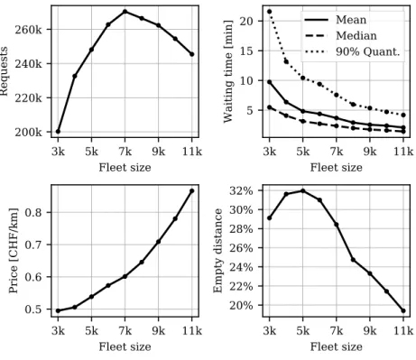
The focus of the thesis is the development of the methodology and the necessary tools. Their application to the use case of Zurich, Switzerland, leads to new insights on AMoD systems when customer perception is considered. In particular, a demand curve can be obtained, which shows that very small or very large fleet sizes are not attractive to the customers.
In the first case, waiting times explode, while in the latter one, the service becomes too expensive. The simulation study yields7,000vehicles as the fleet size that can attract the largest demand. With the fleet control policy chosen, a substantial increase in VKT can be observed, and a consistently higher level of moving vehicles throughout the day. The simulations indicate that care must be taken when setting up policies for future automated vehicle services.
In the last part of the thesis, similar simulations are presented for Paris to demonstrate the transferability of the approach.
iii
Z U S A M M E N FA S S U N G
Automated Mobility on Demand (AMoD) beschreibt ein Konzept, bei dem automatisierte (selbstfahrende) Fahrzeuge zur Personenbeförderung wie die heutigen Taxis eingesetzt werden. Da die Fahrzeuge nicht von Men- schen gesteuert werden, ist zu erwarten, dass die Servicekosten radikal sinken. Gleichzeitig sind solche Dienste sehr attraktiv, da der Zwang ein Fahrzeug zu besitzen entfällt. Negative Auswirkungen wie eine Zunahme der Strassennutzung aufgrund von Leerfahrten der Fahrzeuge oder eine allgemeine Zunahme der Fahrten (induzierte Nachfrage) werden jedoch in der Literatur aktiv diskutiert. Während sich bisherige Analysen und Sim- ulationen auf die Steuerung und Koordination von automatisierten Taxis konzentrieren, gibt es nur wenige Untersuchungen, die die Attraktivität des Dienstes für den Kunden berücksichtigen.
Die vorliegende Arbeit hat das Ziel, diese Forschungslücke zu schliessen, indem drei Komponenten genutzt werden: eine repräsentative Umfrage, die die wichtigen Tradeoffs bei der Verkehrsmittelwahl zwischen konven- tionellen und automatisierten Verkehrsmitteln aufzeigt; ein detaillierter Rechner für die Kosten von Mobilitätsdienstleistungen; und eine agenten- basierte Verkehrssimulation. In dieser Simulation wählen die Reisenden ihre Verkehrsmittel beispielsweise auf der Grundlage der Reisezeit, der Wartezeit und der Kosten aus. Gleichsam hängen aber die Wartezeiten und Kosten rekursiv von der angezogenen Nachfrage ab.
Der Schwerpunkt der Arbeit liegt in der Entwicklung der Methodik und der notwendigen Tools. Die Simulationen für den Anwendungsfall Zürich führen zu neuen Erkenntnissen über AMoD-Systeme, bei welchen die Kundenwahrnehmung berücksichtigt wird. Insbesondere kann eine Nach- fragekurve erstellt werden, die zeigt, dass sehr kleine oder sehr grosse Flot- tengrössen für die Kunden nicht attraktiv sind. Im ersten Fall explodieren die Wartezeiten, während im zweiten Fall der Service zu teuer wird. Die Simulationsstudie ergibt 7.000 Fahrzeuge als die Flottengrösse, die die grösste Nachfrage anziehen kann. Mit dem gewählten Ansatz der Flottens- teuerung ist eine erhebliche Zunahme der Fahrtdistanz und ein konstant höheres Niveau an aktiven Fahrzeugen über den Tag hinweg zu beobacht- en. Die Simulationen zeigen dass bei der Entwickling von Richtlinien für künftige automatisierte Fahrzeugdienste Vorsicht geboten ist.
v
A C K N O W L E D G E M E N T S
Little did I know what an amazing time the following years were to become when I first climbed Hönggerberg. They have passed in the blink of an eye - because of all the extraordinary and wonderful people I have met. This is the place to acknowledge them.
To begin, I want to thank Prof. Axhausen, who gave me the freedom and support to test good (and bad) ideas and to set up my own research agenda.
Thanks for letting me take part in the IVT adventure and allowing me to connect with researchers from all over the world.
Of course, the past years would not have been such a fantastic memory without my fellow PhD students, many of who have transformed from strangers to colleagues to good friends. Thank you all for the productive discussions, coffee breaks and “enlightening” evenings. In particular, I want to mention Felix, who introduced me to the black magic of choice modelling, and Chris, who one day will write a research plan. Without you I would never have spent every dinner in the campus canteen - but also would never have had so much fun!
A big thanks goes to Milos, who never got tired discussing ideas with me; some of the better ones are documented below. Together, we not only went through the ups and downs of MATSim research but also travelled the world. Without you (and your bonus points) those trips to Washington, Porto, Athens, Sydney, Auckland, ... would not have been the same. I hope that many mighty years of working together are yet to come!
About a year after the start of my PhD, I met an ambitious researcher who was brave enough to build on my early work with MATSim. Since then, a large variety of joint research has emerged, much of which is referred to in this thesis. Thank you, Claudio, for the most brilliant remarks and discussions. Good luck on your next adventure!
To finish, I want to thank my parents Yvonne and Mario, my sister Lena and the rest of my family who do not see me as often as they surely deserve.
Thank you for always supporting me on my never-ending journey far from home. Ihr seid die besten! Finally, thank you Maéva, for supporting me every day, for tolerating my hours of “just one more line of code”, and for lovingly reminding me from time to time that a coffe and a walk outside can be equally enjoyable. Je t’aime!
vii
C O N T E N T S
1 i n t r o d u c t i o n 1
1.1 Automated Mobility on Demand . . . 1
1.2 Operational challenges . . . 3
1.3 Automated mobility in Switzerland . . . 4
1.4 Challenges and research goals . . . 6
2 d y na m i c d e m a n d s i m u l at i o n 9 2.1 The MATSim Framework . . . 9
2.1.1 Basic concepts . . . 10
2.1.2 Decision-making in MATSim . . . 13
2.2 Discrete Choice Modeling . . . 22
2.2.1 Basic theory . . . 22
2.2.2 Econometric value . . . 25
2.2.3 Choice sampling . . . 26
2.3 Discrete Mode Choice for MATSim . . . 28
2.3.1 Model structure . . . 30
2.3.2 Model compatibility . . . 36
2.3.3 Further use cases . . . 38
2.4 Discussion and lessons learned . . . 38
2.4.1 Approaches in comparison . . . 38
2.4.2 Fixed error terms . . . 40
3 au t o m at e d m o b i l i t y s i m u l at i o n 43 3.1 Automated vehicles in MATSim . . . 46
3.1.1 Compatibility with discrete choice . . . 49
3.1.2 Further components . . . 51
3.2 The AMoDeus framework . . . 52
3.2.1 Aspects of fleet control . . . 53
3.2.2 Use cases . . . 55
4 z u r i c h m o d e l 57 4.1 Scenario synthesis . . . 58
4.1.1 Available data . . . 59
4.1.2 Algorithms . . . 61
4.2 Cutting process . . . 67
4.2.1 Population . . . 69
4.2.2 Public transport and road network . . . 71
4.2.3 Households and Facilities . . . 73 ix
4.3 Baseline model . . . 75
4.3.1 Custom components . . . 75
4.3.2 Travel behaviour . . . 76
4.3.3 Validation . . . 81
4.4 AMoD Model . . . 84
5 r e s u lt s 89 5.1 Fleet sizing . . . 91
5.2 Scenario analysis . . . 92
5.3 Futher context . . . 98
5.3.1 Dispatching algorithms . . . 99
5.3.2 Pooling potential . . . .102
5.4 Discussion . . . .103
6 t r a n s f e r a b i l i t y 107 6.1 A MATSim scenario for Île-de-France . . . .110
6.2 Case study: Automated taxis in Paris . . . .113
7 g e n e r a l d i s c u s s i o n 119 7.1 Applicability of methods and tools . . . .119
7.2 Open data and software . . . .123
8 c o n c l u s i o n 127
b i b l i o g r a p h y 129
L I S T O F F I G U R E S
Figure2.1 MATSim Zurich . . . 10
Figure2.2 MATSim simulation loop . . . 11
Figure2.3 Queue and buffer . . . 13
Figure2.4 Discrete mode choice structure . . . 31
Figure2.5 Trip-based vs. tour-based mode choice . . . 33
Figure3.1 Automated taxi schedule . . . 48
Figure4.1 Secondary location assignment . . . 66
Figure4.2 Scenario cutter: Trips . . . 69
Figure4.3 Scenario cutter: Network routes . . . 70
Figure4.4 Map of Zurich scenario . . . 74
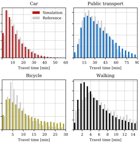
Figure4.5 Calibration: Travel times . . . 82
Figure4.6 Calibration: Travel distances . . . 83
Figure4.7 Calibration: Travel speeds . . . 84
Figure4.8 Calibration: Mode share by distance . . . 85
Figure4.9 Calibration: Mode share by time of day . . . 85
Figure4.10 Classification of road types . . . 86
Figure4.11 AMoD simulation structure . . . 88
Figure5.1 AMoD fleet sizing . . . 91
Figure5.2 AMoD scenarios: Moving vehicles by time of day . . 96
Figure5.3 AMoD scenarios: Accessibility . . . 97
Figure5.4 Control policies: Waiting times . . . .100
Figure5.5 Control policies: Empty distance . . . .101
Figure6.1 General structure of the scenario pipeline. . . .109
Figure6.2 MATSim Île-de-France . . . .111
Figure6.3 Paris AMoD: Operating area . . . .113
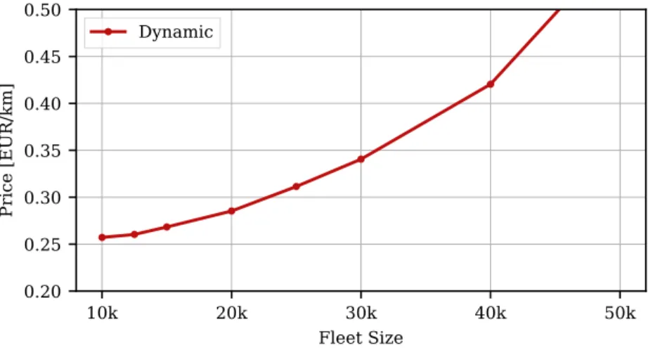
Figure6.4 Paris AMoD: Demand by fleet size . . . .116
Figure6.5 Paris AMoD: Price by fleet size . . . .117
Figure6.6 Paris AMoD: Waiting time by fleet size . . . .118
Figure6.7 Paris AMoD: Fleet activity by time of day . . . .118
xi
Table4.1 MATSim runtimes and memory . . . 68
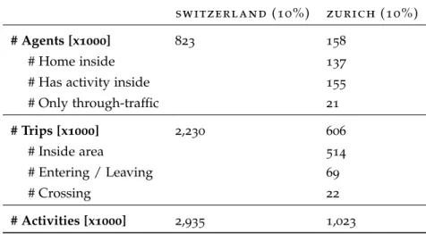
Table4.2 Scenario cutter: Popualtion characteristics . . . 71
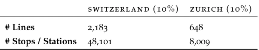
Table4.3 Scenario cutter: Schedule characteristics . . . 72
Table4.4 Scenario cutter: Network characteristics . . . 72
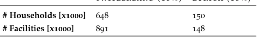
Table4.5 Scenario cutter: Households and facilities . . . 73
Table4.6 Zurich mode choice parameters . . . 78
Table4.7 Basic cost model for Switzerland . . . 80
Table4.8 Subscription cost model for Zurich . . . 80
Table4.9 AMoD mode choice parameters . . . 87
Table5.1 AMoD scenarios: Mode shares . . . 93
Table5.2 AMoD scenarios: Vehicle distance . . . 94
Table5.3 AMoD scenarios: Unique vehicle counts . . . 95
Table5.4 AMoD scenarios: Daily cost and travel time . . . 96
Table6.1 Île-de-France mode choice parameters . . . .114
xii
A B B R E V I AT I O N S
a m o d Automated Mobility on Demand
a r e Federal Office for Spatial Development (Switzerland) au Adaptative Uniform Rebalancing Policy (Section5.3.1) av Automated vehicle
b av Federal Office of Traffic (Switzerland) b f s Federal Statistical Office (Switzerland) b p e Service and facility census for France c h f Swiss Francs
d m c Discrete mode choice (Section2.2, Section2.3)
d r i e a Regional representation of the Ministry of Ecology and Energy in Île-de-France
d r t Demand-Reponsive Transit
d v r p Dynamic Vehicle Routing Problem
e g t Regional household travel survey for Île-de-France e n t d National household travel survey for France e u r Euro
g b m Fluidic Feed-Forward policy (Section5.3.1)
g a General subscription (for public transport in Switzerland) g b m Global Bipartite Matching Policy (Section5.3.1)
g i s Graphical Information System g t f s General Transit Feed Specification
h a f a s Digital public transport schedule for Switzerland
xiii
h t s Household Travel Survey (see MTMC, EGT, ENTD) i n s e e Statistical Office of France
l b h Load-Balancing Heuristic policy (Section5.3.1) m at s i m Multi-Agent Transport Simulation
m t m c Mobility and Transport Micro Census in Switzerland o d Origin-Destination
o s m OpenStreetMap
p r n g Pseudo-Random Number Generator s p Stated Preference (survey)
s tat e n t Enterprise census of Switzerland s tat p o p Population census of Switzerland s v i Association of Swiss transport engineers v k t Vehicle kilometres travelled
v t t s Value of Travel Time Savings (Section2.2.2)
1
I N T R O D U C T I O N
In recent years the world has seen a substantial increase in new mobility solutions. The variety spans from car-sharing services to ride-sharing plat- forms and micro-mobility services which flood cities with electric bikes and scooters. All of these developments have in common that they are fostered by modern information technology, which establishes a quick and convenient communication gateway between customers and service providers.
Along with this, travel decisions are in the process of becoming more and more fast-paced and individual. Traditionally, the options for mid- and long-range trips consisted of car use (which was mainly governed by ownership) or use of more or less well-developed public transit systems.
Today, additional on-demand options exist, which do not require ownership of a mobility tool, but merely membership with various private mobility providers, i.e. ride-sharing services such as Uber, Lyft or any of the numer- ous regional options. They make it easy to call a ride at any time and any location in the service area. Today, a chauffeur-driven vehicle would arrive soon after the request and bring the customer to their desired destination.
Such services offer previously unknown flexibility in terms of space and time, especially for non-car owners.
1.1 au t o m at e d m o b i l i t y o n d e m a n d
At the same time, technology for automated driving is developing at a quick pace. Therefore, studies predict that existing on-demand ride-sharing services will transform into a concept described asAutomated Mobility on Demand(AMoD). Such a service would send robotic taxis to pick up and drop off customers.
One can divide the short-term effects of automated mobility and AMoD into three categories: access to mobility, infrastructure usage and demand effects.
Automated vehicles would allow previously impeded or excluded user groups to gain access to mobility (Litman,2020). This is true for the elderly or young children (Truong et al.,2017) who depend on public transport 1
or other people to drive them, especially in areas that are currently un- derserved by public transport. On the other hand, giving people access to such services could lead to increased individualisation of traffic, which, in turn, might further contribute to the decline of aggregated public transport services.
In terms of infrastructure, some studies predict a more efficient use of the built environment (Alessandrini et al., 2015; Soteropoulos et al., 2019). As many expect automated vehicles to be connected, higher reaction rates could lead to smoother traffic (e.g. Stern et al., 2018) and highly efficient intersections (Pereira et al.,2017;Rios-Torres and Malikopoulos, 2017). Effectively, road capacities would increase, although this may not be true in the early phase of technology adoption as automated vehicles may be required to drive very carefully (see a review inLivingston et al., Upcoming). The flip side, when looking at infrastructure usage, would be that automated vehicles could drive empty. An AMoD system would even depend on empty rides (just like taxi drivers need to go to their customers today) to offer the service. Consequently, the vehicle kilometres travelled (VKT) may increase (Litman,2020) and if an AMoD trip replaces each of today’s private car trips an increase of the number of cars being on the road at any time of day seems likely. In case AMoD could not be operated as efficiently as commonly expected, transport planners may start to observe occupancy rates of less than one person per vehicle at times.
Economically, the crucial point for the feasibility of an AMoD service is its costs. While services such as Uber today are believed to be only kept alive by venture capital, the removal of driver’s wages from the operator’s cost structure may make on-demand ride-sharing services profitable (Bliss, 2018). The prices could then drop drastically, making an AMoD service competitive compared to private vehicle ownership or even public transport.
In such a case, it seems likely that low costs will lead to an increase in individual road-based travel, which is commonly known as the problem of induced demand (Litman,2017;Meyer et al.,2017).
As one crucial competitive advantage of AMoD over private car own- ership, usually comfort is named (seeBecker and Axhausen(2017) for a review of surveys). Automated vehicles may be designed very differently than today’s cars which aim at providing comfort while driving, not for relaxation. Since people can perform many activities other than driving in an automated vehicle, they may value the time spent in the vehicle much higher than today (Becker and Axhausen,2017). While this argument seems to be inherent to automated mobility and AMoD, service quality (such as
1.2 o p e r at i o na l c h a l l e n g e s 3
waiting times and response times) and service costs are strongly dependent on the service provider.
The ecological aspects, welfare considerations and cost-benefit compo- nents of AMoD services are therefore governed by the interplay of efficiency gains and losses in infrastructure use, their relative attractivity compared to traditional modes of transport, and their potential to increase mobility in absolute terms.
1.2 o p e r at i o na l c h a l l e n g e s
From the perspective of the service provider, an AMoD system poses new challenges in fleet control. While traditional transport service planning considers the time scale of years, months or weeks, a fleet of automated ve- hicles can theoretically be controlled dynamically from minute to minute or second to second. It is essential to control vehicle movements, customer pick- ups and dropoffs, maintenance, and charging periods as optimally as possi- ble to gain competitive advantages over other services. For that, the best possible knowledge about the current and future demand is paramount.
Contrary to existing on-demand services that still rely on human interac- tion (König and Grippenkoven,2017), an efficient AMoD system can not be controlled on a per-second time horizon by human dispatchers. Therefore, powerful algorithmic fleet operating policies are vital for the success of an AMoD service. They can make the difference between waiting times of one or two minutes between two different fleet operators.
For the operator, two key questions are essential to assess the profitability and economic sustainability of the service: How much revenue does the service generate by attracting demand? Moreover, how much cost is due to capital and operational expenditures? While longer-term decisions deter- mine capital expenditures (e.g. how many vehicles to include in the fleet), operational expenditures can be almost directly derived from the distance driven by the fleet vehicles. Likewise, the distance driven with a paying customer determines revenues. Therefore, to increase profit or offer lower prices, the empty distance must be minimised.
On the other hand, demand is not only attracted by low prices, but also by low waiting times. While waiting times can be decreased by longer- term decisions (as a higher number of vehicles increases the chances of having one available in due time for every request), this is also possible through short-term fleet management. If the operator can predict demand reliably, he can move idle vehicles towards areas where requests will be
likely to arrive in the future. While he can provide short waiting times for those customers, these vehicles need to be moved empty. Hence, low waiting times come to the cost of extra empty distance, which translates to additional cost for the operator. Fleet operating policies, therefore, need to consider the tradeoff between minimisation of empty distance and not pushing waiting times beyond a guaranteed or desired level.
1.3 au t o m at e d m o b i l i t y i n s w i t z e r l a n d
In2016, the projectSVI2016/001: Induced demand by automated vehicles(Hörl et al.,2019) was commissioned by the Association of Swiss Transport Engi- neers (SVI) and financed by the Federal Road Administration of Switzerland (ASTRA). The project was conducted at the Institute for Transport Planning and Systems at ETH Zurich and had the goal to shed light on several open questions around automated vehicles. The overaching question was how they would affect future mobility in Switzerland. This thesis draws from the results and methods of this project. While the project, in general, looked at both the effects of privately owned automated vehicles and Autonomous Mobility on Demand, the thesis focuses on the results of the latter. The results are complemented by additional research and studies that were inspired by the work inSVI2016/001.
The project consisted of three parts: A detailed cost assessment of au- tomated mobility services in Switzerland, a stated preference survey to estimate user behaviour for automated mobility, and a transport simulation to assess system impacts holistically. The following paragraphs shall give a short overview of the two former components of the project, while the latter part will be the focus of the thesis.
The cost assessment part of the project has lead to a well-received cost calculator of automated and electrified mobility services (Bösch et al.,2018).
The approach of the study was to establish a bottom-up cost assessment of existing mobility options such as private car ownership, public transport or taxi services in Switzerland. The assessed cost components range from investment costs, depreciation and maintenance to cleaning and fuel costs.
The resulting cost values have been validated against known numbers, for instance, from public transport operators. Afterwards, the impacts of automation and electrification on all cost components have been estimated based on the literature. As a result, new cost structures arise which, for instance, take driver wages out of the equation if taxi services replace human-driven cars by automated vehicles.
1.3 au t o m at e d m o b i l i t y i n s w i t z e r l a n d 5
For Switzerland, the study finds that the full cost of owning and using a private car is0.48CHF/pkm. An automated private car, according to this study, is expected to be even more expensive with 0.50 CHF/pkm.
Furthermore, a cost reduction of around 50% can be expected for bus services, while rail services would only be affected marginally. The most substantial cost reduction, however, is expected for taxi services. Today, they are costly in Switzerland with2.73CHF/pkm per passenger kilometre, while an automated taxi service could operate at 0.41 CHF/pkm. This number gets very close to the cost of driving a private car.
The second part ofSVI2016/001started with a survey in the canton of Zurich with about350respondents. In the first phase of the survey, the study asked respondents to provide sociodemographic information about themselves such as age, gender and income and to define two trips they do regularly, one for a distance of less and one for a distance over50km.
In the second phase of the study, all respondents obtained information on automated mobility services, and they had to perform various choice tasks. Those contained their regular trip as indicated before and alternative automated modes of transport such as a private automated car and an automated taxi service. Attributes like waiting times and costs (based on the calculator) were varied to explore how the respondents would opt for or against different automated mobility services in the constructed tradeoff situations. The survey results were subsequently used to estimate statistical models of the respondents’ choice behaviour. From such models, it is possible to calculate a Value of Travel Time Savings, which quantifies how much money a person would theoretically be willing to pay to reduce travel time by, for instance, one hour.
For private cars, the study yielded a VTTS of around19CHF/h while the public transport value is9 CHF/h1. In comparison, travellers value reducing time in an automated taxi at about13CHF/h. Hence, the results indicate that people perceive automated taxis as more comfortable than private cars. Their VTTS are even closer to those of public transport than to the private car. However, in-vehicle time is not the only important factor. In terms of waiting time, the respondents perceive public transport waiting time at 22CHF/h. In contrast, waiting for an automated taxi translates to around35CHF/h. Therefore, people seem to be much more sensitive to long waiting times in an AMoD service than in conventional public transport.
1 For distances of around5km
These results are valuable as they support various assumptions about AMoD. The survey part of the study supports the claim that travellers per- ceive the time spent in an automated taxi as more desirable than spending time in a private car. Adding the removal of the vehicle ownership burden, this renders an AMoD service very attractive compared to private vehicle ownership. Likewise, the cost part of the study confirms that the prices of an AMoD service would be close to car ownership. Hence, it becomes evident that there is a market for AMoD services once the technology is mature enough. Therefore, AMoD operators will likely emerge.
While these results show that AMoD may become an attractive business, it is not clear which impact these services will have on the transport system once they become widely adopted. They may improve or worsen traffic problems in cities, they may or may not be an ecological addition to the transport ecosystem (Taiebat et al.,2018;Wadud et al.,2016), and they may or may not make access to transport more equitable and affordable for everybody. The critical task for transport planning is to assess the potential impact of AMoD services and to study potential outcomes and policy measures (Milakis et al.,2017). Hence, the goal of research should be to inform policymaking on the topic of automated mobility. The third part of SVI2016/001describes simulations to advance such discussions.
1.4 c h a l l e n g e s a n d r e s e a r c h g oa l s
As outlined above, AMoD services require highly dynamic decision making.
On the side of the customer, requests are issued on demand, while the AMoD operator needs to react to those requests in due time. Accordingly, spatially and temporally detailed interactions need to be considered when assessing the value and threats of such a system.
Traditionally, transport researchers use four-step models with which they simulate traffic on a macroscopic level by distributing vehicle flows over a network of roads. The underlying demand is usually defined over spatial zones from fine-grained grids to municipalities or even higher levels of aggregation. In any case, it is not easily possible to consider waiting times in the system, which depend on the specific locations and temporal order of customer requests. However, to allow for a fair assessment, waiting times should affect the choice between AMoD and other modes, just like travel times on congested roads affect the mode choice between public transport and the private car.
1.4 c h a l l e n g e s a n d r e s e a r c h g oa l s 7
Therefore, agent-based transport models have been a common choice for simulations of automated taxis (seeNarayanan et al. (2020) for a recent review). In such models, each traveller and each vehicle is a single entity in the transport network. Therefore, agent-based models appear to be the right choice for simulating emerging mobility modes. They are suited for the simulation of concepts such as automated vehicles, urban air mobility, car-sharing or micro-mobility where availability and attractivity of the service has a highly dynamic spatial and temporal dependency on demand itself. One such agent-based transport simulation frameworks is MATSim (Horni et al.,2016), which is developed by researchers at ETH Zurich and TU Berlin. MATSim was used as the simulation tool inSVI2016/001.
The goal of the remaining project was then to extend and prepare MAT- Sim for the simulation of automated taxi fleets. For that, the simulations made use of the cost analyses and surveys from the previous stages of the study.
The main research questions of the project were:
• How muchdemandwould an automated taxi fleet attract in Zurich?
• How would such a fleetaffectthe transport system in Zurich?
While many simulation attempts for automated taxis existed already at the beginning of the project, none of them took cost structures and user preference into account in a consistent way. Therefore, besides the transport planning-related questions, the development of a methodology to make use of the cost analyses and choice models in MATSim was the technical focus of the project.
The first chapters of this thesis follow the development of the simulation platform. In Chapter2MATSim will be introduced. A comparison between the traditional approach of decision making in MATSim and a novel ex- tension that considers discrete choice models is made. Chapter3covers new simulation components for MATSim that make it possible to simulate automated vehicles. It furthermore gives details on the AMoDeus simula- tion framework that emerged from this work and serves as a comparison platform of fleet control algorithms.
While the development of new simulation components was necessary to reach the project goals, it was equally important to generate a realistic population of artificial agents that represent the travel demand in the study area of Zurich, Switzerland. The synthesis of this population is described in detail in Chapter4. Chapter5then presents results based onSVI2016/001 by analysing how a fleet of automated taxis would affect the transport
system of Zurich. The chapter presents further studies that have partly been done in parallel or after this work to put the obtained results into perspective.
The development of the simulation components and the population synthesis raised many questions and points for discussion. One major point is how far a methodology for agent-based simulation is specific to one use case and whether it can be generalised. Chapter 6covers this topic by showcasing the development of a synthetic agent population for Île- de-France, followed by a simulation of automated taxis in Paris. Finally, Chapter7discusses the applicability of the generated results and tools. The thesis finishes with a conclusion in Chapter8.
2
D Y N A M I C D E M A N D S I M U L AT I O N
The goal of the simulations in this thesis was to explore the interplay be- tween the characteristics of conventional and new mobility services with traveller preferences. This process is inherently circular. Given a specific de- mand, the AMoD operator can provide a certain level of service. If demand increases and the operator does not increase fleet size or uses the vehicles more efficiently, the level of service will worsen. Hence, there is an upper limit of how large the demand can become before waiting times become bad enough that no new customers can be attracted. On the way to this upper demand bound self-selection effects can lead to the phenomenon that different user groups are attracted to the service, depending on the specific configuration of waiting times and prices. Therefore, an important part of the transport simulation should be to simulate such customer behaviour reliably.
The following two sections will give an overview of the MATSim simula- tion framework in general, with a focus on how the simulation considers decision-making. Afterwards, a new decision-making component for MAT- Sim is introduced that makes use of discrete choice models, followed by a discussion of advantages and disadvantages of both approaches. Potential pathways of combining the approaches will be provided.
2.1 t h e m at s i m f r a m e w o r k
MATSim (Horni et al.,2016) is an agent-based transport simulation frame- work. While it can be used as a stand-alone tool with a simple GUI and well-documented configuration file, its real value lies in the fact that it is provided as an open-source programming framework. It provides a rich toolkit to set up very customised and individualised agent-based transport simulations. Occasionally, institutes around the world add new develop- ments to the core code of MATSim ascontributions.
9
Figure 2.1: Example of a MATSim simulation of Zurich with the aim to approx- imate traffic patterns that can be observed in reality. Visualization created in Simunto Via.
2.1.1 Basic concepts
MATSim simulates traffic by treating each traveller and vehicle in the transport system as a unique entity. The simulation is usually performed on a time scale of seconds, which makes it possible to follow locations and states of those entities (agents) in detail throughout one simulation day (see Figure2.1for an example). The goal is then to set up the simulation in a way such that the emerging traffic patterns from interactions of these agents resemble what users observe in reality.
MATSim runs are usually full-day simulations. Each of the simulated agents holds sociodemographic attributes and a daily plan that contains activities and trips. Activities have a specific type, end times and desired durations while trips carry their transportation mode and additional in- formation on the planned route through the transportation network. The basic idea of MATSim is then to simultaneously simulate all of these daily plans in one capacitated transportation network. Traffic jams emerge if too many agents use a particular road in the network. Also, trains can become crowded if too many agents want to use them. From these mobility
2.1 t h e m at s i m f r a m e w o r k 11
Initial Scenario
Mobility Simulation
Decision Making
Analysis
Figure 2.2: The general simulation loop of MATSim with an initial population state, mobility simulation, decision-making and analysis.
simulations, information like the observed travel times, delays and costs for each agent can be recorded. Based on this data, agents can alter their daily plans at the end of the day, for instance in terms of the departure times from activities, their chosen transport modes, the routes through the road network or connections in public transport. Even locations of activities (Horni et al.,2009) or the existence of certain activities themselves may be subject to change (Feil,2010). Afterwards, MATSim simulates the new daily plans with new outcomes.
The two main components of MATSim (as shown in Figure2.2) are a detailed agent-based mobility simulation and a decision-making process.
While the latter will be covered in detail further below, a short overview of the mobility simulation shall be given in the next paragraphs.
The transport simulation part of MATSim comprises two components:
the activity queue and the mobility simulation. Together both components are known as theQSim. At the beginning of one simulation day, all agents rest in activity state. Usually, the first activity in an agent’s plan is a “home”
activity. As each of the agents may have different departure times from the first activity, all agents are put in an ordered queue dependent on their planned activity end time. The QSim then runs iteratively through one full day and checks second by second (or at another configurable interval) which agents should end their current activity. The simulator sends those
agents to update their state. In case they had another activity planned at the same location, theQSimwould add their new activity back to the activity queue, and would wake up the agent again at the activity end time.
However, usually agents would connect activities by trips. Dependent on the desired mode of transport, agents are sent to specific simulators for public transport, slow modes, car travel, and other modes. An important simulator is theNetsim, which simulates car traffic in a queue-based fashion.
TheNetsimis often characterised as a mesoscopic traffic simulator. It does not consider second-by-second movements of vehicles using a car-following model, which would be called microscopic in this context. However, it considers agent interactions on a detailed temporal and spatial level, which goes beyond more aggregated (macroscopic) modelling approaches that rely on volume-delay functions and similar approaches. Internally, the Netsimmodels eachlink(road) in the network as a “queue with buffer” (see Figure2.3). The first part (queue) receives vehicles from upstream, while the second part (buffer) sends vehicles to downstream links. During the simulation, theNetsimconsiders each link individually in two phases for each simulation step.
• In the first phase, vehicles are moved from the queueto the buffer.
Whenever a vehicle enters a link, the Netsim calculates its earliest exit time, based on the traversal speed and the length of the link. It then adds agents to a queue in the order of arrival. Agents at the top of the queue whose exit time is reached are moved further to the buffer. However, certain restrictions exist. In general, all links are characterised by aflow capacity value which defines how many vehicles are allowed to traverse the link per time step. Hence, the link simulator meters how many vehicles it moves to the buffer. Note that this metering is independent of the earliest exit time.
• In the second phase of theNetsim, it moves vehicles from upstream buffers into downstream queues. This movement is only possible if there is space available on the downstream links. This condition is characterised by thestorage capacity, which depends on the length of the link. It describes how many vehicles are allowed to reside on it at the same time. Note that this includes vehicles inside the queue and buffer alike. Hence, traffic is not only limited by theflow capacity, but also by congestion on downstream links.
Agarwal et al. (2018) describe these traffic dynamics in more detail and extend them with additional elements. For instance, the concept of
2.1 t h e m at s i m f r a m e w o r k 13
Link 1 Link 2
Queue Buffer Queue Buffer
Flow Capacity
Storange capacity
Downstream Upstream
Figure 2.3: Schematic visualization of thequeueand thebuffercomponents of road links in MATSim. Theflow capacitydetermines how many vehicles can traverse a link in a defined period. Thestorage capacitylimits the amount of vehicles on the entire link.
holes propagating back from the end of each link allows for more realistic modelling of shock waves inside of the traffic dynamics.
Researchers have applied MATSim to many uses cases around the world in terms of study areas and application domains. There exist well-documented simulation scenarios for Berlin (Ziemke et al.,2019) and Santiago de Chile (Kickhöfer et al.,2016) and studies range from minibus systems (Neumann et al.,2015) to public transit network design (Manser et al.,Under Review), rail interruptions (Leng and Corman,2020), freight simulation (Bean and Joubert,2018), and parking (Bischoff and Nagel,2017) to car-sharing (Ciari et al.,2015;Balac et al.,2019a) and Urban Air Mobility (Balac et al.,2019b).
2.1.2 Decision-making in MATSim
The decision-making process in MATSim is iterative in that always new information is gained from sequential traffic simulations that inform the available choices for the agents. Futhermore, it is based on the theory of utility maximisation. Throughout one day, every activity and trip is valued with a certainscorein MATSim. This score increases if activities are
performed for the right duration and at the right time of day. It decreases if agents are too late or too early or while they spend time in traffic.
A typical score for a trip in an agent’s plan follows the function:
Si=βASC,m
+βtravelTime,m·xtravelTime
+βdistance,m·xdistance +βcost·xcost
(2.1)
Here the β are scoring parameters for the chosen mode m, e.g. m ∈ {car, public transport, bicycle, walk}, andxare attributes estimated or de- rived from the transport simulation. While the parameters in Equation 2.1are standard in MATSim and users can easily set them up through a configuration file, in theory arbitrarily complex scoring functions can be defined in the code.
Note that theβparameters are usually smaller or equal to zero to penalise time spent in transit. Further standard parameters for specific modes, such as aβnumberOfTransfers for public transport are available.
The typical way of scoring activities in MATSim is S+ =βperforming·θtypicalDuration·log xduration
θzeroUtilityDuration
!
(2.2) if the activity is performed for longer than a durationθzeroUtilityDuration. This value may be defined per activity type via configuration but even more fine-grained via code. For shorter durations, the function is linearly extended with the slope at this time, i.e.
S−=−(θzeroUtilityDuration−xduration)· ∂S
∂xduration(0) (2.3) Further scoring components can be applied out-of-the-box. For instance, there is a linear penalty on the time that an agent is arriving too late or leav- ing too early from an activity. Some of these components are furthermore dependent on attributes of the selected location, for instance, opening times of a shop and others. The total score of a realised plan in the transport simulation is then the sum of all trip and activity scores.
After the simulation, it is possible to modify the plan. For instance, an agent may choose a new mode of transport. Withi describing a certain realisation of the daily plan, one can then check how the scores Si of
2.1 t h e m at s i m f r a m e w o r k 15
different realisations relate to each other. In general, utility maximization suggests that a person would prefer planiover planjifSi >Sj.
Assuming that an agent only has access to using the car or public trans- port and the simulation only considers mode choice, we arrive at a countable set of possible plans. Assuming that the plan hasNtrips, there are 2N al- ternative plans. Assuming further that everything else except the agent’s mode choices in the system stays constant, we could simply iterate through all optionsi∈ {1, ..., 2N}and find the best plan as
i∗ =arg max
i
Si (2.4)
In MATSim, many agents are simulated in the transport system. Hence the choice of one agent in the fight for slots in space and time influences the observed score of every other agent. Letl∈N≥1define the index of an agent andL∈N≥0the number of agents. Let furthermoreIlbe the set of all possible plans for agentlsuch thatil ∈ Il. We can then define
I∗= (i∗1, ...,i∗l, ...,i∗L) (2.5) with
Si∗l ≥Sil ∀il ∈ Il ∀l∈ {1, ...,L} (2.6) as a selection of plans in which the system is inuser optimumstate. In this state, none of the agents can improve their score by unilaterally changing their plan.
There are cases in which finding a user optimum is quite easy. Consider the example from above, only that the road network has a limited capacity.
One would start by letting all agents use uncapacitated public transport.
Subsequently, one agent after another would switch to the car alternative as it is valued slightly better. At some point, the road would reach the capacity limit. For all remaining agents, the public transport alternative would then provide a better score. This assignment process is independent of the order of agents if they all have the same perception (i.e. same scoring function).
Hence, there is a large number of possible user optimaIu∗ withu∈ N≥0
describing the different permutations.
Defining S∗l,u as the score of agent l in user optimum u this example would yield that there is a constant valueS∗l,u=C+for all statesuin which agentslare able to use the car, and a constant valueS∗l,u =C−in case they choose the second-best option.
A metric on the scores of all agents can be defined, for instance the total score SSu = ∑lS∗l,u or the mean Su = 1L∑lS∗l,u. Again, in the presented example one would arrive at
SSu=ξC1+ (1−ξ)C2=C3 and Su=C3/L (2.7) where the capacity of the road influencesξ. Nevertheless, both metrics are independent of the specific equilibrium stateu.
Now consider that some of the agents value public transport less than others (maybe because it is not easily accessible for the elderly). In this case, it matters which agent is assigned a specific plan alternative. If all penalised agents need to take public transport, there is the lowest possible SSu. If all of them can take the car, the best possible state is achieved. There are many mixed states in which only a share of those agents can use the car. Note that in any case, all of these states are user equilibria in which agents can not unilaterally improve their score. To gain a better score, two of the “mismatched” agents would need to switch, which is not a unilateral decision. The last considerations add another component to the choice process. From all user equilibrium statesu, is it possible to find theu∗ with
u∗=arg max
u
SSu ? (2.8)
Such a user equilibrium maximises the cumulative or average score of the population. Note that this is still different from asystem optimum in general terms. In a system optimum some agents wouldhavethe possibility to switch to another plan to unilaterally improve their score but they would not do it or they would be prevented from doing so to have an overall better system state. A system optimum is therefore inherently linked to some overall objective (such as minimisation of emissions or low congestion levels) that is policy-defined.
The decision-making process in MATSim has the goal to find a state close tou∗. The aim is to find plan configurations for all agents such that the cumulative population score are as high as possible. Assuming again the toy example from above, where each agent has 2N plan alternatives, the full set of possible configurations of the population would consist of 2N·Lalternatives as one can combine any plan with any other set of plans.
Suppose the plans have three trips, and there are only one hundred agents, there would already be 2300alternatives to evaluate.
The goal of decision making is to give agents freedom in at least two dimensions: departure time choice and mode choice. As outlined above,
2.1 t h e m at s i m f r a m e w o r k 17
givenMdifferent modes of transport andNtrips, an agent may haveMN alternatives to assign modes to trips in their plans. For departure time choice, consider that the agent may choose any hour of the day, so there would be 24N alternatives. Each of them could be combined with each mode choice alternative, leading to(24·M)Noptions. More fine-grained temporal choice options would further increase this number1. Assuming the usual number of four modes in a MATSim simulation and plans of a length of around three trips, this leads to 884, 736 alternatives, which is closer to what would be the case in a realistic simulation. Now consider that MATSim intends to simulate thousands or even millions of agents, which would mean one needs to evaluate(884, 736)1,000,000 alternatives to find the optimal user equilibrium. A further explosion of alternatives can be observed when there are thousands of locations that serve as alternative destinations for the activities in the plans.
Evaluating all possible configurations is not an option for all practical applications of MATSim. Therefore, an approach is used that has been coined as the “co-evolutionary algorithm” of MATSim. The algorithm consists of four major parts: (1) scoring agents’ plans as described above, (2) the plan memory, (3) plan selection, and (4) innovation strategies.
At the beginning of a MATSim simulation, each agent usually starts with one initial plan that is scored in the subsequent mobility simulation.
Afterwards, this plan may be modified, but modifications are not applied directly to the existing plan. Instead, the algorithm copies the plan and applies changes to this copy. Both the original plan and the newly generated one are then part of theagent memory. The memory has a limited size in the magnitude of around three to five plans and tracks the observed score for each plan. If a new plan exceeds the memory limit, the algorithm chooses one of the plans to be removed.
Copying and modifying an existing plan is only one option that can happen after the mobility simulation. MATSim defines a set ofreplanning strategieswhich define the decision-making of the agent. Each of the strate- gies kis assigned a certain weight wk, which defines the probability of calling this strategy in the replanning step of MATSim. For that purpose the weights are normalized such that∑kwk =1.
There areselection strategiesandinnovation strategies. The former consider the memory of an agent and apply a specific selection procedure to choose one of the plans to be executed in the next iteration. Note that the “re- membered” score of a plan might not be up to date anymore because the
1 In fact, in MATSim any second of the day could be chosen.
conditions in the transport system may have changed. This way, the score of the selected plan is updated after the next mobility simulation run.
Theinnovation strategieshave the task to apply modifications to a copied plan. The typical modules areTimeMutator, which changes the activity end times in the plan with a random offsetδsampled from a uniform distri- bution ∆∼ U(−T,T),Reroute, which updates a trip’s route through the network, andSubtourModeChoice. The latter searches for all trip sequences in a plan that start and end at the same location. Then, the strategy changes the transport modes of these trips to randomly chosen alternatives. For modes that are not constrained by mobility tools (like making sure that the private car arrives back home), further fine-grained randomisation of modes along the sequence is possible in recent versions of MATSim.
Structurally, thereplanningstep of MATSim looks as follows:
ifmemory exceeds limitthen Choose plan for removal
ifremoved plan was selected plan of agentthen Uniformly select new plan
Choose replanning strategy based on weights ifa selection strategy is chosenthen
Apply strategy to select a plan for execution ifa innovation strategy is chosenthen
Uniformly select one plan from memory Add a copy of the plan to memory
Apply changes to it acc. to innovation strategy Select new plan for execution
Two design decisions strongly influence the behaviour of the algorithm:
the selection strategy for plan removal and the plan selection strategy. The standard configuration of MATSim always removes the plan with the worst score. The set of plans in memory is therefore implicitly biased towards plans with higher scores.
One common choice for plan selection is to use the logit formula. Denot- ing the plans in an agent’s memory byP1, ...,PNthe probability of selecting planPiis
2.1 t h e m at s i m f r a m e w o r k 19
P(Pi) = exp(σSi)
∑Ni0=1exp(σSi0) ( 2.9) According to the formula, plans with higher scores are selected with higher probability. Note that usuallyσis set to 1. Together with the magni- tude ofSit has considerable influence how “random” the selection is. In caseσ=0 the selection would be uniform over the available plans, while σ→∞would make the selection deterministic for the plan with the highest score2.
The usual plan selector in MATSim mimics the behaviour of the logit formula, but only considers a choice between the currently selected planP∗ with scoreS∗and one uniform randomly selected plan from memory. The probability of switching from the currently selected plan to the proposed plan P0 with scoreS0is then:
P(P∗→P0) =ηexp(β(S0−S∗)) (2.10) One can interpret the formula as follows: If S∗ = S0 the probability of performing the transition is η. If S∗ > S0 the probability is smaller thanηand if the proposed plan has a better score, the probability of the switch is larger thanη. Currently,η is fixed toη =0.01 in MATSim, but should probably be made available through configuration in the future.
Theoretically, this selection process converges to the same results as the logit formula (Nagel and Flötteröd,2016). The choice ofηdoes not affect this statement; rather, the speed of convergence is dependent on it.
Other plan selectors are available, such as a uniform random selector and a “maximum score selector”, which always selects the best plan that is available in memory. It will become of interest further below.
The search dynamics from iteration to iteration have two major influences:
The repeated removal of the worst plan, and preference of selecting plans with high scores. As the innovation part proposes changes at random, the selection and removal parts are responsible for filtering out those proposals that are not beneficial to increase the agent’s daily score. The reason for not always selecting the plan with the maximum score and keeping a memory of past plans is to be able to escape local maxima. While a particular plan may have been updated multiple times with increasing score, it may reach a limit eventually. In that case, it makes sense to jump back to a plan from
2 This is only true in theory. In practice large numbers ofσwould lead to loss of numerical precision and overflow.
before and “try” a different path of modifications that may lead to better results.
This search for the user equilibrium comes with artefacts: Imagine a search process as described above that runs for infinite time, but there are no capacity restrictions in the system (i.e. anybody can choose between car or public transport). In such a case plans with the slightly better scored car choice would accumulate in all agents’ memories over time. Now and then, the innovation step would produce a plan where the agent has to use public transport. As MATSim would call the innovation strategy with replanning weightw(for instance in10% of the cases,w=0.1) there would be a50/50chance to create a “car” or a “public transport” plan. Hence, in expectation, one would see at least5% of agents in the simulation taking public transport.
The recommended remedy for such a search artefact is to turn off in- novation strategies after a sufficient number of iterations. After that, only selection is active on all agents’ memories. For some of them, a sub-optimal plan may still exist, but dependent on the scores of the optimal plans the rate of occurrence after selection might be low.3However, for practical pur- poses, simulations cannot be run for such large numbers of iterations that optimal plans sufficiently populate agents’ memories. Accordingly, innova- tion turn-off will “freeze” the current memory of an agent and afterwards selection is performed on this set of plans.
The situation becomes more complicated if there are capacities in the simulation. Then each agent’s optimal score is dependent on the plans of all other agents. Having10% of agents innovating their plans heavily biases the perceived situation in the transport system. Therefore, turning off innovation has another objective in this, more practice-relevant, case: By re- moving10% of strongly random (and potentially irrational and unintuitive) travel decisions, traffic conditions are stabilised substantially. Accordingly, it becomes easier to bring the agents into an equilibrium state,giventhe plans that are available to them after turning off innovation. However, even then, one can observe variability in the choices from iteration to iteration as the selection process remains stochastic.
To summarise, MATSim applies a search algorithm which uses random plan changes to generate plan proposals in a user equilibrium. The selection and removal part chooses those proposals that are promising to lead to a high score equilibrium. As the search space is vast and computational
3 It will likely not be zero, except maximum score selection is used.
2.1 t h e m at s i m f r a m e w o r k 21
resources are limited, the process stops once the population reaches a sufficiently stable score.
At the end of this analysis, the focus should be put again on the initial question: How does decision-making in MATSim work? MATSim strongly revolves around the concept of a user equilibrium in which every agent finds a daily plan with the best possible score. One can criticise this approach from different perspectives. First, one can argue that reality is inherently not in equilibrium. Constantly, decisions and conditions are changing. However, we observe phenomena such as traffic jams that occur every morning at the same spots in a city. It is therefore also possible to argue that some constrained situations, in reality, are close to a user equilibrium. Indeed, the selfish behaviour of travellers plays an active role in causing congestion.
Second, assuming that one can sufficiently approximate reality by a user equilibrium, which one is the correct one? Is it the one with the highest possible “cumulative score”, the one with the lowest, or somewhere in between? While these are interesting questions, they are of lesser practical relevance in setting up MATSim simulations.
The reason is that it is inherent to the process that one needs to calibrate MATSim. Usually, one does this by setting scoring parameters in such a way that specific metrics obtain a good fit with reference data measured from reality. The most common of such metrics is the overall mode share of the system. In the toy example, we would measure that in reality,70% of travellers take the car and30% of them take public transport. Interestingly, if the system does not have any capacities, turning off innovation at the right point becomes crucial even to be able to achieve such a modal split. Other calibration objectives are vehicle counts on specific links for an average weekday or by the hour, boarding and alighting counts at public transit stations or travel time distributions, to give some examples.
At the time of writing this thesis, multiple approaches for automatic calibration of MATSim simulations have been proposed (Flötteröd et al., 2012) or are under development (Makarova et al., Under Review). The recently published Opdyts algorithm (Flötteröd,2017) makes use of the iterative structure of MATSim as system metrics and scores can be approx- imated by a linear increase between two or few iterations. Interestingly, innovation turn-off poses a problem in such cases as it introduces a strong non-linearity into the model dynamics. It is therefore important to discuss potential alternatives.
In the future, it will be essential to study some of the phenomena men- tioned above and to describe the search process of MATSim more thor-
oughly: How does the variance within one simulation depend on the chosen parameters? How does the variance across simulations with different ran- dom seeds behave? How does turning off innovation at different iterations affect the final score and variance? Some of such analyses have recently performed on specific use cases (Guggisberg Bicudo,2020;Paulsen et al., 2018), but not formalized in a general way.
2.2 d i s c r e t e c h o i c e m o d e l i n g
Discrete mode choice models (Train,2009) are an essential part of transport research. It is their goal to statistically describe the decisions that people make, for instance, when they are faced with the task to decide whether to take a car to go to work or to take the bus. The nature of most of the decisions of interest is discrete, i.e. there are two or more options available that comprise specific attributes. The following section will give a brief introduction to set the field for understanding how a discrete mode choice model has been integrated into MATSim.
2.2.1 Basic theory
Most discrete choice models are based on the concept of utility maximiza- tion. While MATSim is focused around the notion of maximizing a score, discrete choice models assume that decision-makers want to maximize theutilityof their decision. Similar to scoring functions in MATSim, those systematic utilities are expressed analytically:
vi,car=βASC,car+βtravelTime,car·xtravelTime,car,i+βcost·xcost,car,i+...
vi,pt=βASC,pt+βinVehicleTime,pt·xinVehicleTime,pt,i
+βwaitingTime,pt·xwaitingTime,pt,i+βlineSwitch,pt·xlineSwitches,pt,i
+βcost·xcost,pt,i...
(2.11)
Here,videscribes the utility of an alternative for decisioni,xdescribe the choice attributes andβare the model parameters that define the tradeoffs between the attributes and alternatives. Each alternative has a specialβASC, which is the alternative specific constant. Note that parameters can appear multiple times, likeβcost, which describes how monetary costs are perceived.
2.2 d i s c r e t e c h o i c e m o d e l i n g 23
Allβcan be thought of as being given in the unit of utilities[utls/·]and are combined in the vectorβ.
Assume that there are N persons and each of them has been tracked for one day. The trip of interest is their morning commute. Each morning commute then represents a choice situationi, here between two different modes “car” and “public transport”. Furthermore, the attributes x are known for all chosen and alternative options. Given tripiand alternativek, we can define a deterministic utilityvi,k(β).
Definingk∗i as the selected alternative of all respondents, we can try to find a set ofβthat fulfil the following constraint:
k∗i =arg max
k
{vi,k(β)|k∈ {car,pt}} ∀i∈ {1, ...,N} (2.12) Generally, this will not easily be possible as some choices by different respondents may be contradictory in the sense of Equation2.12. Such dif- ferences exist because people have variable tastes in their decision making, and the utility functions defined by the modeller may only approximate the choice process in all its subtlety. Therefore, slack is added to the utilities by explicitly modelling uncertainty about the choice into the equations. We define a random utility for each choice situationiand alternativekas:
ui,k =vi,k+σei,k (2.13) Here,ei,kis a i.i.d. random variable andσ∈R≥0. We now require that:
k∗i =arg max
k
{vi,k(β) +σei,k|k∈ {car,pt}} ∀i∈ {1, ...,N} (2.14) The selected choicek∗i can now be expressed as a random variableK∗i that follows a specific distribution, dependent on the error distribution. Some alternatives are more likely to be chosen than others. Note that ifσ=0 the random term vanishes and deterministic choices are made, but ifσ→∞ the random term becomes dominant. Hence, choices would be completely random. It is possible to formally write down the probability that a certain alternativekiis the actual choicek∗i in choice situationi:
P(Ki∗=ki| β) =P(ui,ki ≥ui,1∧...∧ui,ki ≥ui,K| β) (2.15) The probability ofki being the selected option is the probability of its associated utility being larger or equal to the utility of any other choice.