Research Collection
Doctoral Thesis
Coupling Finite Elements and Auxiliary Sources
Author(s):
Casati, Daniele Publication Date:
2020-03
Permanent Link:
https://doi.org/10.3929/ethz-b-000386816
Rights / License:
In Copyright - Non-Commercial Use Permitted
This page was generated automatically upon download from the ETH Zurich Research Collection. For more information please consult the Terms of use.
Diss. ETH No. 26522
Coupling Finite Elements and Auxiliary Sources
A thesis submitted to attain the degree of DOCTOR OF SCIENCES of ETH ZURICH
(Dr. sc. ETH Zurich) presented by DANIELE CASATI MSc ETH CSE, ETH Zurich
born on 04.06.1990 citizen of Italy
accepted on the recommendation of Prof. Dr. Ralf Hiptmair, ETH Zurich, examiner
Prof. Dr. Jasmin Smajic, Hochschule f¨ur Technik Rapperswil, co-examiner Prof. Dr. Igor Tsukerman, University of Akron, co-examiner
2020
Coupling Finite Elements and Auxiliary Sources
ISBN: 978-3-906916-80-4 DOI: 10.3929/ethz-b-000386816 ETH Dissertation Number: 26522
Funding: Swiss National Science Foundation (Grant No. 2000021 165674/1) c 2020 Daniele Casati
Abstract
We propose a hybrid method to solve time-harmonic Maxwell’s equations inR3 through the Finite Element Method (FEM) in a bounded region encompass- ing parameter inhomogeneities, coupled with the Multiple Multipole Program (MMP) in the unbounded complement.
FEM and MMP enjoy complementary capabilities. FEM requires a mesh of the computational domain of interest. This is expensive, but can treat inho- mogeneous materials, shapes with corners, or other singularities. Moreover, FEM allows a purely local construction of the discrete system of equations.
On the other hand, MMP belongs to the class ofmethods of auxiliary sources and of Trefftz methods, as it employs point sources that are exact solutions of the homogeneous equations as (global) basis functions: one only needs to evaluate them on hypersurfaces to obtain the discrete problem, and the resulting linear combination is valid in the whole domain where the equations hold, which can be unbounded. MMP performs well where the electromagnetic field is smooth, i.e. in the free space far from physical sources and material interfaces.
Thus, a natural way to combine the strengths of these methods arises when one needs to simulate the electromagnetic field of components with inhomogeneous parameters or nonsmooth shapes surrounded by free space: use FEM on a mesh defined on the components and MMP in the unbounded domain outside.
The boundary between the FEM and MMP domains can be nonphysical if one surrounds the components by a conforming mesh of an “airbox” also modeled by FEM.
The interface conditions on the surface of the FEM domain are key to accurate coupled FEM–MMP solutions. Integrating by parts the variational form solved by FEM, surface integrals appear, through which one can impose interface conditions by substituting the ansatz of MMP.
trace for Maxwell’s equations) cannot be imposed in this way.
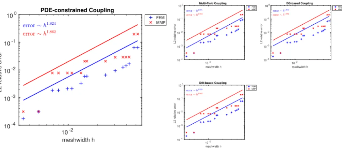
To include this additional condition, we derive four methods from Lagrangian functionals that enforce both the variational form in the FEM domain and all the interface conditions between different discretizations:
1. Least-squares-based coupling using techniques fromPDE-constrained op- timization. This approach optimizes a functional for the additional con- dition, subject to a constraint expressed by the variational form of FEM.
2. Discontinuous Galerkin (DG) between the meshed FEM domain and the single-entity “MMP mesh”, interpreting MMP as FEM with special basis functions.
3. Multi-field variational formulation in the spirit of mortar finite element methods, relying on the same interpretation of MMP as the DG-based coupling.
4. Coupling through the Dirichlet-to-Neumann operator: here we intro- duce a weak formulation of the additional condition where MMP basis functions are used as test functions. This approach is generalized to couple MMP with any numerical method based on volume meshes that fitsco-chain calculus.
Furthermore, to minimize the meshed region and for the sake of generalization, we assume that equation parameters are piecewise constant in the MMP do- main (instead of constant everywhere). This induces a partition: we consider the case of one unbounded subdomain with other bounded, but possibly very large, subdomains, each requiring its own MMP discretization space (but with- out the need of meshes). Hence, on top of the interface conditions between the FEM and MMP domains, one should also impose interface conditions between the MMP subdomains themselves.
We compare the FEM–MMP coupling approaches in a series of numerical experiments with different geometries and equation parameters, including ex- amples that exhibit triple-point singularities. Convergence tests are performed for examples that cover the whole spectrum of computational electromagnet- ics, obtaining the expected results.
Riassunto
Proponiamo un metodo ibrido per risolvere inR3 equazioni di Maxwell armo- niche nel tempo tramite ilmetodo degli elementi finiti (FEM) in una regione limitata caratterizzata da parametri disomogenei, accoppiato col programma dei “multipoli multipli”(Multiple Multipole Program, MMP) nel complemento illimitato.
FEM ed MMP offrono caratteristiche complementari. FEM richiede una mesh del dominio di interesse. Ci`o `e dispendioso, ma permette di trattare materiali disomogenei, figure con spigoli o altre singolarit`a. Inoltre, con FEM si pu`o costruire localmente il sistema di equazioni discreto.
D’altra parte, MMP appartiene alla classe dei metodi delle sorgenti ausilia- rie e dei metodi di Trefftz, dato che utilizza come funzioni di base (globali) delle sorgenti puntiformi che sono soluzioni esatte delle equazioni omogenee:
per ottenere il problema discreto si deve valutarle solo su ipersuperfici, e la combinazione lineare risultante `e valida nell’intero dominio di validit`a delle equazioni, che pu`o essere illimitato. MMP funziona bene quando il cam- po elettromagnetico `e regolare, ovvero in spazio libero da sorgenti fisiche e interfacce di materiali.
Si ha quindi un modo naturale di combinare i punti di forza di questi metodi quando si vuole simulare il campo elettromagnetico di componenti con para- metri disomogenei o forme non lisce circondate da spazio libero: si usi FEM su una mesh definita sulle componenti ed MMP nel dominio illimitato esterno. Il bordo tra i domini FEM ed MMP pu`o non essere fisico se si circondano le com- ponenti con una mesh conforme di una “scatola d’aria”, anch’essa modellata da FEM.
Le condizioni di interfaccia sulla superficie del dominio di FEM sono cruciali per ottenere soluzioni accoppiate tra FEM ed MMP. Integrando per parti la forma variazionale risolta da FEM, appaiono integrali di superficie con cui si possono imporre condizioni di interfaccia sostituendovi l’ansatz di MMP.
traccia tangenziale per equazioni di Maxwell) non pu`o essere imposta in questo modo.
Per includere questa condizione aggiuntiva, deriviamo quattro metodi da fun- zionali di Lagrange che impongono sia la forma variazionale delle equazioni nel dominio di FEM, sia tutte le condizioni di interfaccia tra discretizzazioni differenti:
1. Accoppiamento basato sui minimi quadrati tramite tecniche di ottimiz- zazione con vincoli dati da equazioni alle derivate parziali. Questo ap- proccio ottimizza un funzionale per la condizione aggiuntiva soggetto ad un vincolo espresso dalla forma variazionale di FEM.
2. Galerkin discontinuo (DG) tra la mesh di FEM e la “mesh di MMP”
formata da una sola cella, se si considera MMP come un metodo agli elementi finiti con funzioni di base speciali.
3. Formulazione variazionale multicamponello spirito dei metodi degli ele- menti finiti mortar, che si affida alla stessa interpretazione di MMP su cui si fonda l’accoppiamento basato su DG.
4. Accoppiamento tramite l’operatore Dirichlet a Neumann: introducia- mo una formulazione debole della condizione aggiuntiva dove funzioni di base MMP sono usate come funzioni test. Questo approccio si pu`o ge- neralizzare per accoppiare MMP con qualsiasi metodo numerico basato su mesh di volume che rientri nelcalcolo delle cocatene.
Inoltre, per minimizzare la regione con mesh e per generalizzare, assumiamo che i parametri delle equazioni sianocostanti a tratti nel dominio MMP (invece di costanti ovunque). Ci`o induce una partizione: consideriamo il caso di un so- lo sottodominio illimitato assieme ad altri sottodomini limitati, che comunque possono essere molto grandi, ciascuno col proprio spazio di discretizzazione MMP (ma senza bisogno di mesh). Dunque, in aggiunta alle condizioni di interfaccia tra i domini FEM ed MMP, si devono anche imporre condizioni di interfaccia tra gli stessi sottodomini di MMP.
Paragoniamo i modi di accoppiare FEM ed MMP in una serie di esperimenti numerici con diverse geometrie e parametri delle equazioni, inclusi esempi che esibiscono singolarit`a di punto triplo.
Eseguiamo test di convergenza per esempi che coprono l’intero spettro dell’e- lettromagnetismo computazionale, ottenendo i risultati sperati.
Acknowledgments
This thesis would not have been possible without the support and guidance of my supervisor, Prof. Ralf Hiptmair, to whom I am very grateful. I would also like to thank my co-supervisor Prof. Jasmin Smajic for his encouragement, especially his help in building collaborations, my co-supervisor Prof. Christian Hafner for sharing valuable expertise from his long academic career, as well as the external co-examiner Prof. Igor Tsukerman.
This work was supported by a grant from the Swiss National Science Founda- tion under project 2000021 165674/1.
Contents
Acronyms xiii
1 Preliminaries 1
1.1 Boundary Value Problems . . . 1
1.1.1 Poisson’s Equation . . . 1
1.1.2 Helmholtz Equation . . . 2
1.1.3 Maxwell’s Equations . . . 3
1.1.4 Eddy-Current Model . . . 4
1.2 Domain Decomposition . . . 5
1.3 Function Spaces . . . 7
1.4 Finite Elements . . . 10
2 Trefftz Methods 13 2.1 Trefftz Spaces . . . 13
2.2 Multiple Multipole Program . . . 15
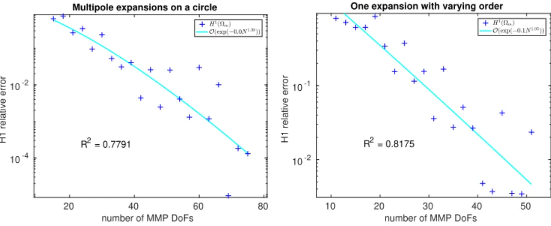
2.3 Trefftz Approximation Error in 2D . . . 19
2.3.1 Numerical Results for the Poisson’s Equation . . . 21
2.3.2 Numerical Results for the Helmholtz Equation . . . 24
2.4 Trefftz Approximation Error for Maxwell’s Equations . . . 27
3 Coupling Strategies 31 3.1 PDE-constrained Least-Squares Coupling . . . 32
3.1.1 Poisson’s Equation . . . 32
3.1.2 Maxwell’s Equations . . . 35
3.2 Discontinuous Galerkin . . . 38
3.2.1 Poisson’s Equation . . . 38
3.2.2 Maxwell’s Equations . . . 40
3.3 Multi-Field Coupling . . . 45
3.3.1 Poisson’s Equation . . . 45
3.3.2 Maxwell’s Equations . . . 48
3.4 DtN-based Coupling . . . 50
3.4.1 Poisson’s Equation . . . 50
3.4.2 Maxwell’s Equations . . . 53
4 Trefftz Co-chain Calculus 55 4.1 Co-chain Calculus . . . 55
4.2 Formalism . . . 57
4.3 Coupling through an (l−1)-Form . . . 58
4.4 Coupling through an (m−1)-Form . . . 62
5 Implementation 65 5.1 Libraries . . . 67
5.2 Executables . . . 69
6 Numerical Experiments 71 6.1 2D Diffusion . . . 72
6.1.1 2D Diffusion with Exact Solution . . . 72
6.1.2 2D Diffusion with Jumping Coefficients . . . 75
6.2 Electrostatics . . . 78
6.3 2D Scattering . . . 80
6.3.1 2D Scattering with Exact Solution . . . 80
6.3.2 2D Scattering with Triple-Point Singularities . . . 87
6.4 Magnetostatics . . . 91
6.4.1 Magnetostatics with Exact Solution . . . 91
6.4.2 Magnetostatic Inductor . . . 95
6.5 Eddy Current withH-Φ Formulation . . . 97
6.6 Maxwell’s Equations . . . 102
6.6.1 Maxwell’s Equations with Exact Solution . . . 102
6.6.2 Maxwell’s Equations with Triple-Point Singularities . . 107
7 Conclusions 115
References 117
Curriculum Vitae 127
Acronyms
BEM Boundary Element Method. xx, xxi, 55, 115 DEC Discrete Exterior Calculus. 56
DG Discontinuous Galerkin. iv, vi, 32, 38–40, 43, 45, 48, 50, 68, 70, 89, 95, 107, 109, 111, 113–115
DoF Degree of Freedom. xv, xvi, 76–78, 89, 91, 107, 109–111, 113, 114 DtN Dirichlet-to-Neumann. xii, xv, xxii, xxiii, 50–53, 55, 61, 67, 70, 84, 95,
97, 100, 102, 103, 115
FEEC Finite Element Exterior Calculus. 56
FEM Finite Element Method. iii–vi, xiii, xvi, xvii, xx–xxiv, 1, 4–7, 11, 14, 29–32, 38–40, 43, 50, 53, 55, 56, 65–69, 71, 72, 74, 76, 78, 81, 83, 84, 86, 87, 89, 92, 95, 97–99, 103–105, 107, 109, 111, 112, 114, 115
MAS Method of Auxiliary Sources. 14, 15
MMP Multiple Multipole Program. iii–vi, xiii, xv, xvi, 13, 15, 17, 19, 20, 22–30, 38, 40, 42, 45, 48, 50, 55, 65–72, 74–76, 78, 80–84, 86–89, 91, 92, 94, 95, 97, 98, 103–107, 109–111, 113, 114
PDE Partial Differential Equation. iv, xi, 11, 14, 15, 32, 33, 35–37, 42, 53, 70, 89, 104, 107, 111, 113–115
TPS Triple-Point Singularity. xv–xvii, xxiii, 25–28, 87–89, 91, 107–114
0Notation.
Subscript f in formulas: FEM.
Subscript m in formulas: Trefftz method (MMP).
Superscriptnin formulas: discrete.
List of Figures
1.1 Physical domains vs. computational domains . . . 6
2.1 Sample multipoles for 2D Poisson . . . 16
2.2 Current loop and closed curve to test Amp`ere’s law . . . 18
2.3 Error plots for 2D Poisson without singularities solved by MMP 22 2.4 Error plots for 2D Poisson with a singularity solved by MMP . 23 2.5 MMP subdomains . . . 23
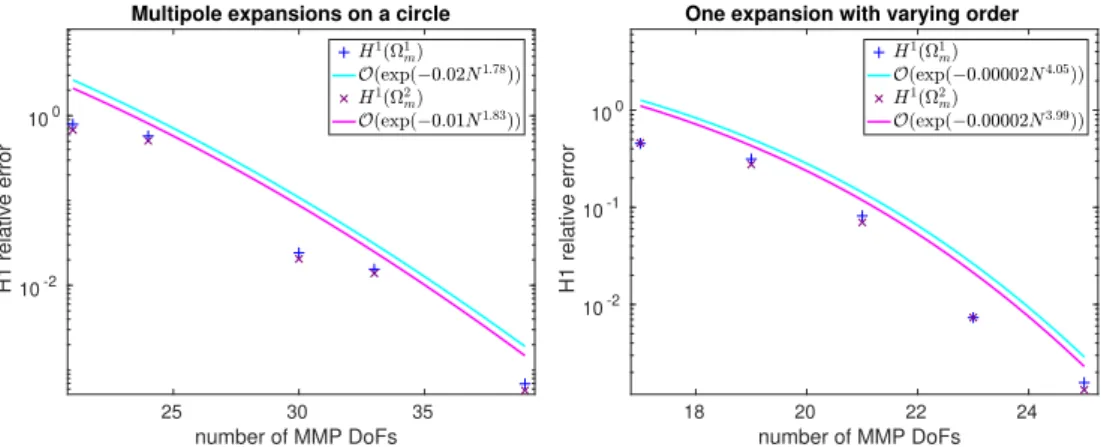
2.6 Error plots for 2D Helmholtz without TPS (k1 =k2 = 1.59k0) solved by MMP . . . 25
2.7 Error plots for 2D Helmholtz with TPS (k1 = 4k0, k2 = 2k0) solved by MMP . . . 26
2.8 Error plots for 2D Helmholtz with TPS (k1 = 100k0,k2= 10k0) solved by MMP . . . 26
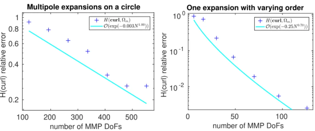
2.9 Error plots for Maxwell’s equations without TPS solved by MMP 28 2.10 Magnitude ofu for photonic nanojet . . . 29
5.1 Sample matrix of DtN-based coupling for 2D scattering . . . . 67
6.1 Geometry of Ωf for 2D diffusion with exact solution . . . 73
6.2 Error plots for 2D diffusion with exact solution . . . 74
6.3 Meshwidth vs. MMP DoFs for 2D diffusion with exact solution 75 6.4 Geometries of Ωf ⊇Ω? for 2D diffusion with jumping coefficients 76 6.5 Error plots for 2D diffusion with jumping coefficients: Ωf = Ω? 77 6.6 Error plots for 2D diffusion with jumping coefficients: Ωf ⊃Ω? (Γ is polygonal) . . . 77
6.7 Error plots for 2D diffusion with jumping coefficients: Ωf ⊃Ω? (Γ is C1) . . . 78
6.8 Geometry of Ωf for electrostatics . . . 79
6.9 Error plots for electrostatics . . . 79
6.10 Meshwidth vs. MMP DoFs for electrostatics . . . 80
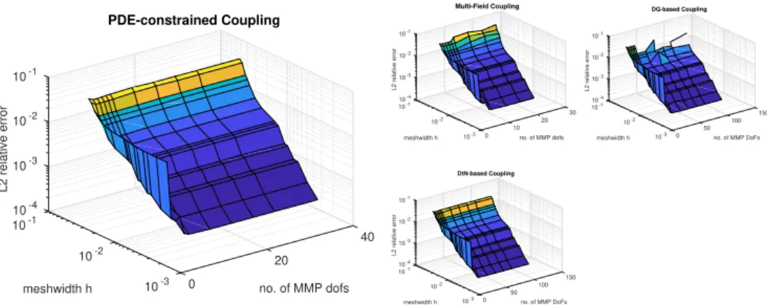
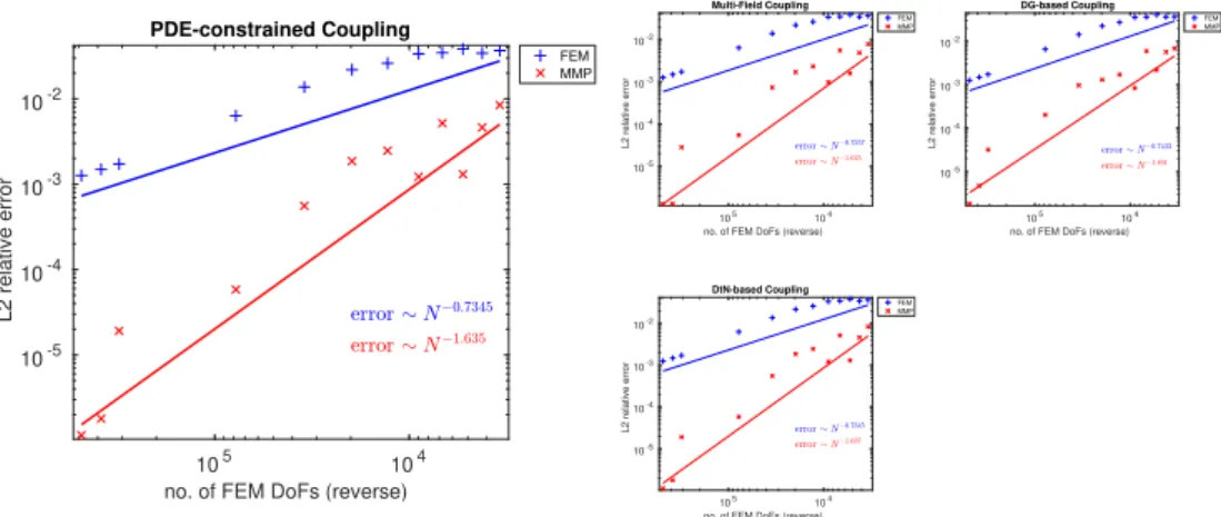
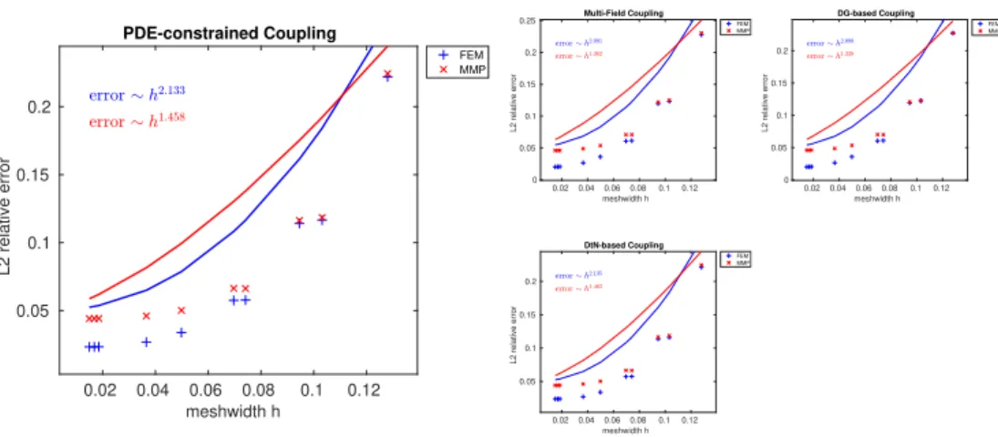
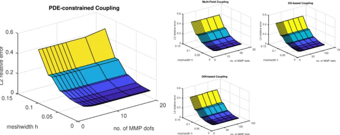
6.11 Error plots for 2D scattering with exact solution (ω= 23.56·107) 82 6.12 Meshwidth vs. MMP DoFs for 2D scattering with exact solution
(ω= 23.56·107) . . . 82
6.13 Error plots for 2D scattering with exact solution (ω= 23.56·108) 83 6.14 Magnitude of Poynting vector for photonic nanojet . . . 84
6.15 Geometry and mesh of Ωf,Ω0m,Ω1mfor 2D scattering with exact solution . . . 85
6.16 Error plots for 2D scattering with exact solution: two MMP domains with one multipole expansion each . . . 86
6.17 Error plots for 2D scattering with exact solution: two MMP domains with many multipole expansions . . . 87
6.18 Geometry and mesh of Ωf,Ω1m for 2D scattering with TPS . . . 88
6.19 Error plots for 2D scattering with TPS (geometry in Figure 6.18a) 89 6.20 Geometry and mesh of Ωf,Ω1m,Ω2mfor 2D scattering with TPS 90 6.21 Error plots for 2D scattering with TPS (geometry in Figure 6.20a) 91 6.22 Mesh of Ωf for magnetostatics with exact solution . . . 92
6.23 Error plots for magnetostatics with exact solution: radius 4 . . 93
6.24 Error plots for magnetostatics with exact solution: radius 2 . . 93
6.25 Meshwidth vs. MMP DoFs for magnetostatics with radius 4 . . 94
6.26 Meshwidth vs. MMP DoFs for magnetostatics with radius 2 . . 94
6.27 Geometry and mesh of Ωf for magnetostatic inductor . . . 96
6.28 Magnitude ofu for magnetostatic inductor . . . 97
6.29 Geometry of Ωf for eddy-current equations . . . 98
6.30 Eddy currents for different mesh refinements . . . 100
6.31 Power loss for different mesh refinements . . . 101
6.32 Error plots for eddy-current equations . . . 101
6.33 Magnitude ofHfor eddy-current equations . . . 102
6.34 Magnitude ofu for Maxwell with exact solution . . . 103
6.35 Error plots for Maxwell with exact solution . . . 104
6.36 Meshwidth vs. MMP DoFs for Maxwell with exact solution . . 105
6.37 Mesh of Ωf,Ω1mfor Maxwell with exact solution . . . 106
6.38 Error plots for Maxwell with exact solution: two MMP domains 106 6.39 Mesh of Ωf,Ω1mfor Maxwell with TPS . . . 108
6.40 Error plots for Maxwell with TPS (µ+ = 4µ0,µ−= 2.5281µ0) . 109 6.41 Error plots for Maxwell with TPS (µ+ = 10µ0,µ−= 4µ0) . . . 110
6.42 Mesh of Ωf,Ω1m,Ω2m for Maxwell with TPS: minimal FEM mesh 110 6.43 Error plots for Maxwell with TPS: minimal FEM mesh . . . 111
List of Figures 6.44 Mesh of Ωf,Ω1m for Maxwell with TPS: minimal FEM mesh &
layered medium . . . 112 6.45 Error plots for Maxwell with TPS (µ+= 4µ0,µ−= 2.5281µ0):
minimal FEM mesh & layered medium . . . 113 6.46 Error plots for Maxwell with TPS (µ+ = 10µ0, µ− = 4µ0):
minimal FEM mesh & layered medium . . . 114
Introduction
Computational electromagnetics is devoted to the numerical simulation of the interactions of the electromagnetic field with the physical world. Compared to the subject of electromagnetism, the focus is on practical applications, rather than the theory.
The well-known Maxwell’s equations in differential form [43, p. 337, (7.40)]
constitute the basis of this analysis. These linear equations look simple and almost symmetric with respect to their unknowns, and present smooth exact solutions where equation parameters are constant (for example, [43, p. 395, (9.43)]). Difficulties arise from complex geometries or local equation param- eters, which can even be nonlinear or subject to a hysteresis loop (see [43, p. 290]); for example, these parameters can have jump discontinuities on the interface between different materials. Hence, the geometry of the components forming the spatial domain is of paramount importance.
Different numerical methods perform best in different circumstances. Methods relying on volume meshes can handle singularities of shapes with corners by locally refining the mesh there, but only work in bounded domains. Other methods only require evaluations on hypersurfaces to obtain a solution that also holds inside volumes, as long as the problem is simple enough, but require to explicitly know the solution of some other related problem in advance (for example, for the homogeneous equation).
A common strategy to simulate real-world applications is to use methods of the first class, which can handle inhomogeneities, with a boundary condition that well approximates the field despite artificially truncating the mesh.
Some boundary conditions are trivial to implement, such as the surface of a perfect electric conductor, where the tangential component of the electric field and the normal component of the magnetic field are set to zero [43, p. 425, (9.175)]. Things become more difficult if the solution is a wave propagating to infinity. In this case, absorbing boundary conditions or perfectly matched
layers can be used [72]. Both, however, are local approximations to nonlocal operators, and therefore have limitations [59, p. 14, Section 7].
Hence, a good strategy is to use both kinds of methods discussed above, based on volume meshes and hypersurfaces, for the same problem, i.e. to devise ahy- brid domain-decomposition method. Domain decomposition refers to splitting the equations into coupled problems on smaller subdomains forming a par- tition of the original domain. To form a hybrid method, this decomposition becomes relevant at the discrete level, where different approximation methods are employed in each subdomain.
The most popular hybrid method is probably the Finite Element Method (FEM) coupled with the Boundary Element Method (BEM): as a famous pa- per states in the title, the marriage of convenience (`a la mode) between these methods can achieve the “best of both worlds” [15]. FEM is not only apt to model inhomogeneous materials, but can also be used without knowing fun- damental solutions of the governing differential equations. These solutions, which BEM requires, can be nonexistent or extremely complex.
On the other hand, BEM is clearly better-suited for domains involving a small ratio of boundary surface to volume: extreme cases are unbounded domains.
Moreover, the coupling of FEM and BEM is not very difficult, as both have their roots in integrations by parts by means of Green’s identities [64, p. 4, (1.8) and (1.9)] (variational form for FEM, boundary integral equation for BEM) and are set in related function space frameworks [8].
However, BEM presents two disadvantages:
1. Singular integrals in its formulation. While one can usually get rid of these singularities (for example, with Duffy transformations or analytic integrals for some geometries of the boundary), an ad-hoc solution per problem has to be identified. This complicates the implementation, which cannot be a “black box”, i.e. valid for any problem involving Maxwell’s equations, as with FEM.
2. More importantly, given that kernels of boundary integral equations are nonlocal, BEM leads to large, dense matrices. A whole set of techniques is devoted to their study (panel-clustering methods orhierarchical matri- ces [75, pp. 464–465, Section 7.6]), but those same matrices still appear
Introduction as blocks of the linear system of equations originating from coupling FEM and BEM.
Thus, we propose to couple FEM with a Trefftz method (Chapter 2) instead of BEM. In fact, Trefftz methods present the following desirable features:
1. No singular integrals, because if Trefftz basis functions have central sin- gularities, they are placed at points outside the Trefftz domain of ap- proximation. When coupled with FEM, these singularities are therefore positioned in the FEM domain.
2. When applied to analytic solutions, the approximation error of Trefftz methodsconverges exponentially. We can formally prove this when Tre- fftz methods are used to model the Poisson’s equation [64, p. 246, Chap- ter 8] inR2 (Section 2.3) and show it empirically for Maxwell’s equations (Section 2.4).
Quoting again the author arguing in favor of the marriage between BEM and FEM [87, p. 314, Section 5],
it seems without doubt that in the future Trefftz type elements will frequently be encountered in general finite element codes. [...]
It is the author’s belief that the simple Trefftz approach will in the future displace much of the boundary type analysis with singular kernels.
Of course, Trefftz methods also have a major flaw, namely their dependence on heuristics, especially impacting the choice of Trefftz basis functions in 3D settings. As a matter of fact, when modeling close to field singularities or sources, the quality of their numerical solutions is heavily impacted by the choice of Trefftz basis functions; e.g., the position of their central singularities inside the FEM domain. An ideal strategy is therefore to apply FEM where the field is difficult to model and Trefftz methods elsewhere, such that heuristics becomes irrelevant. This suggests to use an artificial interface between the FEM and Trefftz domains, not coinciding with any discontinuity of material properties.
Throughout this thesis we show how well the coupling between FEM and Trefftz methods matches the aforementioned expectations through numerical
results covering the whole spectrum offrequency-domain computational elec- tromagnetics.
Scope
Several approaches to couple FEM and a Trefftz method for the Poisson’s equation in both 2D and 3D have been discussed by the author from the per- spective of numerical analysis in [28]. Existence, uniqueness, and stability of all coupling approaches is formally proven in that work, which only deals with scalar unknown functions. We offer numerical evidence for Maxwell’s equations (vector unknown functions) in [29, 30], which illustrate numerical convergence results for the magnetostatic and eddy-current equations, respec- tively.
[26] generalizes one of the coupling approaches, the Dirichlet-to-Neumann- based coupling (DtN-based coupling, Section 3.4), to any numerical method based on volume meshes. The particular case of the coupling with the cell method, a technique based on both a primal and a dual volume mesh [83], is illustrated theoretically and through numerical experiments performed with iterative solvers applied to the Schur complement [18, p. 221] of the coupling systems (Trefftz degrees of freedom are eliminated).
Finally, [27] assumes that equation parameters are piecewise constant in the Trefftz domain, which induces a partition: one unbounded subdomain and other bounded, but possibly very large, subdomains, each requiring its own Trefftz discretization space. Hence, coupling strategies are extended to handle more than one Trefftz domain for the case of 2D Helmholtz equation [64, p. 276, Chapter 9].
The coupling between FEM and a Trefftz method has also been addressed be- fore from an engineering perspective [79]. However, a different methodology for the coupling is used in that work: FEM and Trefftz field values, the Dirich- let data, are matched in selected points on the interface between their domains (collocation method), while the Neumann data enter through a boundary term of the variational form. The resulting overdetermined system of equations is solved in the least-squares sense.
Introduction To the best of our knowledge, apart from these papers, little research has been devoted to the investigation of strategies combining Trefftz methods with con- ventional finite element methods. We cite [45, 71]: in particular, the coupling proposed in [45, p. 672, Section III] is the same as the DtN-based coupling of Section 3.4.
Remark. It is also worth mentioning the infinite element method [39], pri- marily used for exterior Helmholtz problems, which employs standard FEM in a bounded domain and infinite elements in the unbounded exterior. In fact, given a spherical coordinate system [43, p. 38, Section 1.4.1], the radial com- ponent of infinite elements is expressed by a multipole expansion [43, p. 151, Section 3.4], which can be used as Trefftz basis functions (see Section 2.2).
Conversely, the spherical component is approximated by standard polynomial finite element shape functions [67, p. 143, Section 5.6].
Infinite elements are then coupled with standard FEM by solving the varia- tional form of the equations everywhere (see Section 1.4): unbounded radial integrals can be computed by choosing a radial dependence that leads to expo- nential integrals [2, p. 227, Chapter 5]. The final coupling system may not be symmetric.
This thesis describes the coupling techniques introduced in [28, 29, 30, 27] for Poisson’s (one Trefftz domain) and time-harmonic Maxwell’s equations and illustrate all the numerical results reported in these works. Novel results for FEM coupled with more than one Trefftz domain are also included ([27] is confined to 2D Helmholtz).
Having multiple Trefftz domains allows to treat piecewise-constant material parameters on potentially very large regions, while using a minimal volume mesh for the FEM domain. This mesh can be so small that it only surrounds points where the field is singular, likeTriple-Point Singularities (TPS), which emerge at the junction of three different materials [42]. At the same time, one also needs to impose interface conditions between neighboring Trefftz domains, which requires a mesh on the interfaces separating them.
Furthermore, while mesh-based methods like FEM suffer from the well-known pollution effect [9] with time-harmonic Maxwell’s equations, oscillating basis
functions are used in the Trefftz domains (see Section 2.2): these basis func- tions may achieve better approximation properties than the classical piecewise- polynomial spaces of FEM [54].
Outline
Chapter 1 illustrates the boundary value problems discussed in this work. It also provides references to the relevant formalism of functional analysis and, specifically, FEM, one leg of the hybrid strategy we propose. The other leg, Trefftz methods, is more thoroughly described in Chapter 2, where we also present results on the related exponential convergence behavior.
Given these approaches, Chapter 3 describes four algorithms to couple them:
one of these strategies is further generalized in Chapter 4, so that it can couple Trefftz methods with any numerical technique based on volume meshes.
Chapter 5 gives some insight into the code that is used for the numerical ex- periments of this work. The corresponding results are described in Chapter 6, showing the convergence of all coupling approaches with one or more Trefftz domains (that also need to be coupled with each other) and with or with- out an analytic solution: an example of the latter is when singularities are introduced.
Some remarks in Chapter 7 conclude the work.
1 Preliminaries
This chapter illustrates the boundary value problems and notation behind our description of the coupling approaches between FEM and Trefftz methods.
Firstly, the continuous setting: the boundary value problems considered in this work (Section 1.1), including time-harmonic Maxwell’s equations (Sec- tion 1.1.3), the partition of their domain Rd, d= 2,3 (Section 1.2), and the function spaces involved in each subdomain and on the interfaces between them (Section 1.3). Secondly, given all these ingredients, in Section 1.4 we derive the variational (weak) forms of the boundary value problems, which constitute the basis of their discretizations relying on volume meshes, and present thediscrete finite element spaces used in this work.
1.1 Boundary Value Problems
1.1.1 Poisson’s Equation
To derive some theoretical (Section 2.3 and Chapter 3) and numerical results (Sections 2.3.1, 6.1, and 6.2), we refer to the following Poisson’s problem:
− ∇ ·
M−1µ (x)∇u
=j in Rd, d= 2,3, (1.1a)
u(x) =
clogkxk+O(kxk−1) inR2, c∈R
O(kxk−1) inR3 forkxk → ∞ uniformly, (1.1b) which, inR3, models anelectrostatic phenomenon [43, p. 60] throughGauss’s law [43, p. 182, (4.22)] for theelectric displacement field [43, p. 182, (4.21)].
• u: Rd→C,d= 2,3, represents the electric displacement field.
• Mµ: Rd → Cd,d is a symmetric, bounded, uniformly positive-definite matrix that corresponds to an inhomogeneous, anisotropic permeability [43, p. 285, (6.32)]. We assume that Mµ(x) =µI ∀x∈Rd\Ω?, given a bounded domain Ω?⊂Rd, andµ∈Cconstant everywhere inRd\Ω?.
• j: Rd→Crepresents the stationary current that generates the electro- magnetic field. j has compact support in Ω?.
• The decay condition (1.1b) follows from [64, p. 259, Theorem 8.9].
1.1.2 Helmholtz Equation
The numerical results in Sections 2.3.2 and 6.3 are obtained for the reference 2D Helmholtz problem
−∇ ·
M−1µ (x)∇u
−ω2(x)u=j inR2, (1.2a)
∇u·x−ıkkxku= 0 forkxk → ∞ uniformly, (1.2b) which models the scattering of transverse-electric polarized z-invariant time- harmonic electromagnetic waves at penetrable objects [43, p. 427, (9.181)].
• u: R2 → C represents the longitudinal (z-)component of a magnetic vector potential [43, p. 243, (5.61)]
• Mµ: R2→C2,2 is the same permeability of Section 1.1.1, while: R2→ C represents an inhomogeneous permittivity [43, p. 186, (4.33)]. We again assume thatMµ(x) =µI ∀x∈R2\Ω?, given a bounded domain Ω?⊂R2, but this timeµ, ∈Carepiecewise constant inR2\Ω?.
• ω∈Ris the angular frequency [43, p. 386, (9.11)], whilek:=ω√ µthe piecewise-constantwavenumber [43, p. 385, Section 9.1.2] inR2\Ω?.
• j: R2 →Cis the same stationary current of Section 1.1.1.
• (1.2b) is the Sommerfeld radiation condition; please refer to [32, p. 19, Definition 2.4].
1.1 Boundary Value Problems 1.1.3 Maxwell’s Equations
We now consider the following second-order vector boundary value problem for numerical results in Sections 2.4 and 6.6:
∇ ×
M−1µ (x)∇ ×u
−ω2M(x)u+∇φ=j
∇ ·u= 0
inR3, (1.3a)
∇ ×u×x−ıkkxku=0 forkxk → ∞uniformly, (1.3b) which models time-harmonic Maxwell’s equations [43, p. 233, (5.56)] expressed in terms of a magnetic vector potential subject to the Coulomb gauge [43, p. 440, (10.8)].
• u: R3→C3 represents the magnetic vector potential.
• φ: R3 → C represents the electric scalar potential [43, p. 79, (2.23)], which also acts as a Lagrange multiplier to impose the Coulomb gauge.
φmust be subject to a further constrain such that it is uniquely defined by (1.3a). In the scope of this work, we setR
R3φdx= 0.
• Mµ,M:R3→C3,3are symmetric, bounded, uniformly positive-definite matrices that correspond to an inhomogeneous, anisotropic permeability and permittivity, respectively. We assume that both Mµ(x) = µI and M(x) = I ∀x ∈ R3 \Ω?, given a bounded domain Ω? ⊂ R3, and µ, ∈Care piecewise constant inR3\Ω?.
• ω ∈ R and k := ω√
µ are the same constant angular frequency and piecewise-constant wavenumber (in R3\Ω?) of Section 1.1.2.
• j: R3 → C3, with ∇ · j = 0, represents the stationary current that generates the electromagnetic field. jhas compact support in Ω?.
• (1.3b) is theSilver-M¨uller radiation condition; please refer to [32, p. 195, Definition 6.6].
It is implicitly assumed thatk6= 0; otherwise, if, e.g.,ω= 0, we would be in a magnetostatic regime [43, p. 241, Section 5.3.4] – see Section 6.4. In this case,
the Silver-M¨uller radiation condition would be replaced by the decay condition [57, p. 180, (5.28)]
u(x) =O(kxk−1) forkxk → ∞uniformly. (1.4) 1.1.4 Eddy-Current Model
Here we consider a special case of Section 1.1.3, i.e. amagnetoquasistatic [55]
reduced eddy-current [43, p. 310] model obtained from Maxwell’s equations.
We use the H-Φ formulation [63], which employs the H-field [43, p. 279, Sec- tion 6.3] in electrically-conductive [43, p. 296] domains Ωc (≡ Ω? from Sec- tion 1.1.3) and a magnetic scalar potential Φ (see Remark 1.2.1 in the next section) in nonconductive domains Ωn. This form typically requires to know the source magnetic field Hs before simulating and has difficulties with a multiply-connected Ωc (see Remark 1.2.1).
J. Smajic in [78] proposes a newH-Φ field formulation on a multiply-connected domain not requiring to precompute theHs-field before the actual simulation.
Here we present another formulation with the same property and later solve it by coupling FEM and Trefftz methods.
Indeed, let us consider the same eddy-current boundary value problem as in [78], but on an unbounded domain Ωn := Ω+\Ωc, where Ω+ designates the first octant ofR3 (all axes with positive directions). The reason for the octant is that we treat XY,XZ, and Y Z as symmetry planes of our model, where we impose boundary conditions.
∇ × σ−1∇ ×H
+ıωµcH=0 in Ωc n× ∇ ×H=0 on∂NΩc
n×H=0 on∂DΩc H=∇Φ, ∇ ·(µn∇Φ) = 0 in Ωn
n·µn∇Φ = 0 on∂NΩn Φ = I/2 on∂D1Ωn Φ = 0 on∂D2Ωn Φ is const on∂D3Ωn
(1.5)
1.2 Domain Decomposition Φ on∂D3Ωnis a constant potential that has to be determined. For Φ at infinity we aim at the same behavior as (1.4).
We assume that the bounded conductive domain Ωc lies inside Ωf, Ωc ⊆ Ωf, similarly to Ω? in Section 1.2. Hence, given Lemma 1.3.1, interface conditions between Ωc and Ωn (inside Ωf) are required for the field to be well-posed:
n×H=n× ∇Φ
µcn·H=µnn· ∇Φ on∂cnΩc. (1.6a) (1.6a) should be imposed together with the other interface conditions between the FEM and Trefftz domains, also derived from Lemma 1.3.1:
Φf = Φm
n· ∇Φf =n· ∇Φm on Γ, (1.6b)
with Γ lying inside Ωn.
We will solve this problem in Section 6.5, where a geometric model of Ωc, Ωn, and their boundary conditions is provided.
1.2 Domain Decomposition
For Sections 1.1.2 and 1.1.3, piecewise-constantµ, inRd\Ω?,d= 2,3, induce a natural partition ofRd\Ω? intom+1 subdomains Ωi,i= 0, . . . , m, such that the pair (µ, )∈C2 (and therefore the wavenumberk) is constant in each Ωi. We denote the constant wavenumber in each subdomain withki,i= 0, . . . , m, and assume that there is only one unbounded domain in this partition, which we refer to as Ω0.
To simplify the exposition and without loss of generality, from now on we assume that m = 1 for Sections 1.1.2 and 1.1.3, i.e. that Ω0∪Ω1 =Rd\Ω?, with constant k0 ∈ C in the unbounded domain Ω0 and constant k1 ∈ C in the bounded Ω1. Generalization to m > 1 is immediate. For Section 1.1.1, the simpler casem= 0 (one unbounded domain) holds.
Ω٭=supp(μ(x) )
∪ supp(ε(x) )
∪ supp(j)
Ω1 Ω0
non const nonconst
μ1,ε1
μ0,ε0
(a) Sample domains Ω?, Ω0, and Ω1.
Ωf
Γf0
Ω٭=supp(μ(x) )
∪ supp(ε(x) )
∪ supp(j)
Ωm1 Ωm0
Γf1 Γ01
non const nonconst
μ1,ε1
μ0,ε0
(b) Sample domains Ωf, Ω0m, and Ω1m.
Figure 1.1: Physical domains (Figure 1.1a) do not necessarily correspond to computational domains (Figure 1.1b): Γf0,Γf1 can be artificial in- terfaces. Different colors in the (left) figure represent regions with different parametersµ, .
However, for our computations we introduce a different domain decomposition.
As a matter of fact, we do not necessarily have to couple FEM and Trefftz methods across physical interfaces that coincide with discontinuities of param- eters µ, . Hence, instead of considering the physical domains Ω?,Ω0,Ω1 (see Figure 1.1a), we take a different partition for computations (see Figure 1.1b):
Rd= Ωf∪Ω0m∪Ω1m∪Γf0∪Γf1∪Γ01, (1.7) with Γf0:=∂Ωf ∩∂Ω0m, Γf1 :=∂Ωf∩∂Ω1m, Γ01:=∂Ω0m∩∂Ω1m and Ωf∩Ω0m=
∅, Ωf ∩Ω1m = ∅, Ω0m ∩Ω1m = ∅. We also define Ωm := Ω0m ∪Ω1m and Γ := Γf0∪Γf1∪Γ01; for Section 1.1.1, Ωm= Ω0m and Γ = Γf0=∂Ωf =∂Ωm. We demand Ω? ⊆Ωf, but not necessarily Ω? = Ωf. If Ω? 6= Ωf, Γf0∪Γf1 =∂Ωf
is an artificial interface. Note that Ωf can be composed of disjoint regions.
We also demand that Ω0m,Ω1m include different values of the equation pa- rameters of (1.3a): Ωim ⊆ Ωi, i = 0,1, i.e. constant wavenumbers k0, k1 for Ω0m,Ω1m.
We call Ωf, a bounded Lipschitz domain [41, p. 4, Definition 1.1], the FEM domain, whereas Ω0m is the unbounded and Ω1m the bounded Trefftz domain.
The terminology indicates the type of approximation of the unknown to be
1.3 Function Spaces employed in each domain. Coupling between the FEM and Trefftz domains is done across the (artificial) interfaces Γfi,i= 0,1, while coupling between the two Trefftz domains occurs across the physical interface Γ01 (not required for Poisson’s problem of Section 1.1.1).
Remark 1.2.1. A special setting occurs when ki = 0 and Ωim is also simply connected [37, p. 252, Section 8]. As a matter of fact, as Ωim does not con- tain any free current by definition (Ω? ⊆Ωf), then we can replace Maxwell’s equations (1.3a) for k = 0 in Ωim with the Poisson’s problem (1.1) using a magnetic scalar potential[43, p. 245, (5.67)] (see Section 1.1.4) as unknown, which is easier to handle (see Sections 4.4 and 6.5).
1.3 Function Spaces
We look for unknowns u (Sections 1.1.1 and 1.1.2) andφ,u (Section 1.1.3) in Sobolev spaces [67, p. 36, Chapter 3] on a generic open set Ω⊆Rd,d= 2,3:
• H1(Ω) [67, p. 38] for u and H∗1(Ω) :=
v∈H1(Ω) : R
Ωvdx= 0 for φ, and
• H(curl,Ω) [67, p. 55, (3.40)] and the broader Hloc(curl,Ω) for u: the subscript “loc” indicates that functions belong to the reported space, hereH(curl,Ω), after multiplication with a compactly-supported smooth function [67, p. 230].
In the following we will also make use of Sobolev spaces L2(Ω) [67, p. 36, Section 3.2], L2t(∂Ω) [67, p. 48, (3.13)], andH(div,Ω) [67, p. 52, (3.29)].
Given these spaces and the computational domains introduced in Section 1.2, for Sections 1.1.2 and 1.1.3 we can decomposeu, φ,u as
uf:= u|Ω
f ∈H1(Ωf), u0m:= u|Ω0
m ∈Hloc1 (Ω0m), u1m:= u|Ω1
m ∈H1(Ω1m), (1.8a) φf:= φ|Ω
f ∈H∗1(Ωf), φ0m:= φ|Ω0
m ∈H∗,loc1 (Ω0m), φ1m:= φ|Ω1
m ∈H∗1(Ω1m), (1.8b) uf:= u|Ω
f ∈H(curl,Ωf),u0m:= u|Ω0
m ∈Hloc(curl,Ω0m),u1m:= u|Ω1
m ∈H(curl,Ω1m).
(1.8c)
For Section 1.1.1, the decomposition (1.8a) is only on domains Ωf and Ωm= Ω0m.
It is now important to introduce a formalism to evaluate u, φ,u on the in- terfaces Γf0,Γf1,Γ01 between Ωf,Ω0m,Ω1m. The relevant traces [67, p. 42, Sec- tion 3.2.1] are
• theDirichlet trace [67, p. 43, (3.8)],
• theNeumann trace γN [75, p. 68, (2.103)]:
γN:
Hloc1 (∇2,Ω)→He−12(Γ),
v7→n·M−1µ ∇v for v∈Hloc2 (Ω),
(1.9a)
• thetangential trace [67, p. 57, (3.45)],
• thetangential components trace [67, p. 57, (3.46)], and
• themagnetic trace γm [67, p. 59, (3.51)]:
γm:
Hloc(curl curl,Ω)→He−12(divΓ,Γ), v7→n× M−1µ ∇ ×v
. (1.9b)
We define the terms appearing in (1.9a) and (1.9b):
• Ω∈
Ωf,Ω0m,Ω1m and Γ∈ {Γf0,Γf1,Γ01}.
• n is the normal vector on Γ.
• Hloc1 (∇2,Ω) is the space of functions v ∈ Hloc1 (Ω) for which ∇2v ∈ L2loc(Ω).
• He−12(Γ) [67, p. 44] is the dual space [67, p. 19, Definition 2.14] of H12(Γ) [67, p. 44], given by the range of Dirichlet traces. The tilde of He−12(Γ) takes into account that Γ is generally an open interface [75, p. 59, (2.90)].
• Hloc(curl curl,Ω) is the space of functions v ∈ Hloc(curl,Ω) for which ∇ ×(∇ ×v)∈L2loc(Ω) :=
L2loc(Ω)3
.
1.3 Function Spaces
• He−12(divΓ,Γ) [67, p. 59] is the dual space of H−12(curlΓ,Γ) [67, p. 59, (3.53)].
Relying on this formalism, we can then write theinterface conditions that the restrictions of the solution of a generic boundary value problem on two different domains Ω1,Ω2 have to satisfy across the common interface Γ := Ω1∩Ω2 for the joint solution to be well-posed. They are given by [67, p. 107, Lemma 5.3], which we report here, given the importance of these conditions for our work:
Lemma 1.3.1. Let Ω1,Ω2 be nonoverlapping Lipschitz domains [67, p. 38, Definition 3.1] with a common surface Γ := Ω1∩Ω2 with nonzero measure.
• Given u1 := u|Ω
1 ∈ H1(Ω1), u2 := u|Ω
2 ∈ H1(Ω2), and u ∈ L2(Ω1 ∪ Ω2∪Γ), then:
u1
Γ=u2
Γ=⇒u∈H1(Ω1∪Ω2∪Γ).
• Given u1 := u|Ω
1 ∈ H(curl,Ω1), u2 := u|Ω
2 ∈ H(curl,Ω2), and u ∈ L2(Ω1∪Ω2∪Γ), then:
n×u1
Γ=n×u2
Γ=⇒u∈H(curl,Ω1∪Ω2∪Γ).
• Given u1 := u|Ω
1 ∈ H(div,Ω1), u2 := u|Ω
2 ∈ H(div,Ω2), and u ∈ L2(Ω1∪Ω2∪Γ), then:
n·u1
Γ=n·u2
Γ=⇒u∈H(div,Ω1∪Ω2∪Γ).
Hence, for Poisson’s problem (1.1), interface conditions betweenuf := u|Ω
f ∈ H1(Ωf) andum:= u|Ω
m ∈Hloc1 (Ωm), given a single Trefftz domain Ωm (m= 0), with Γ =∂Ωf =∂Ωm, are
uf|Γ = um|Γ, (1.10a)
γNuf|Γ = γNum|Γ. (1.10b) For Helmholtz problem (1.2), interface conditions are the same as (1.10) but for the three interfaces Γf0,Γf1,Γ01 between Ωf,Ω0m,Ω1m:
uf|Γ
fi = uim
Γfi, (1.11a)
γNuf|Γ
fi = γNuim
Γfi, (1.11b)
withi= 0,1. Analogous conditions also have to hold across Γ01.
Finally, the interface conditions that the solution u of (1.3) has to satisfy across Γfi,i= 0,1, are
n×uf
Γfi = n×uim
Γfi, (1.12a)
γmuf
Γfi = γmuim
Γfi, (1.12b)
n·uf
Γfi = n·uim
Γfi. (1.12c)
(1.12a) and (1.12b) stem from the first line of (1.3a), (1.12c) from the second line (Coulomb gauge).1 Analogous conditions also have to hold across Γ01.
1.4 Finite Elements
Integrating Maxwell’s equations over any volumes and surfaces inRd,d= 2,3, and exploiting the divergence [43, p. 31, (1.56)] or Stokes’ theorems [43, p. 34, (1.57)], one obtains theintegral (weak) formof Maxwell’s equations [43, p. 342, Section 7.3.6]. This form, involving fluxes and line integrals, is considered by some [83] to be more “physical” than the corresponding differential form [43, p. 341, (7.56)], as it involves directly measurable quantities, like currents, allows more relaxed smoothness requirements for the unknowns (which can be smooth almost everywhere), and also encodes conservation of energy. For these reasons, Maxwell’s equations in integral form constitute the basis of the cell method [84].
On a similar note, a finite element analysis always starts from thevariational form of the differential equations involved. By testing the integral form of (1.1a) on Ωf with suitable functions and integrating by parts, we obtain
Seek uf ∈H1(Ωf) : Z
Ωf
M−1µ ∇uf
· ∇vf dx− Z
Γ
γNuf vf dS= Z
Ωf
j vf dx ∀vf ∈H1(Ωf). (1.13a)
1At first sight, one could think of combining (1.12a) and (1.12c) and impose the continuity uf
Γfi =uim
Γfi,i= 0,1. However, this would only hold if each restriction ofulay in H1(Ω) :=
H1(Ω)3
.
1.4 Finite Elements
Let us also introduce the variational form for Maxwell’s PDEs (1.3a):
Seek uf ∈H(curl,Ωf), φf ∈H∗1(Ωf) :
R
Ωf
M−1µ ∇ ×uf
·(∇ ×vf)−ω2(Muf)·vf dx+ P
i=0,1
R
Γfiγmuif ·vf dS+R
Ωf∇φf·vf dx=R
Ωfj·vf dx ∀vf ∈H(curl,Ωf), R
Ωfuf · ∇ψf dx− P
i=0,1
R
Γfi n·uif
ψf dS = 0 ∀ψf ∈H∗1(Ωf).
(1.13b) We use standard finite element spaces to discretize (1.13a) and (1.13b) in Ωf ⊇ Ω?, where Mµ,M may vary in space. These discrete spaces are built on triangular [18, p. 65, Section 5.6] (in R2) or tetrahedral meshes Mf [67, p. 112, Section 5.3] on Ωf. More specifically, we discretize uf ∈ H1(Ωf) and φf ∈H∗1(Ωf) with piecewise-linear Lagrangian finite elements [67, p. 143, Sec- tion 5.6], i.e.
Vn(Mf) := S10(Mf) :=
n
vn∈C0(Ωf) : vn|K(x) =aK+bK·x, aK∈R, bK ∈Rd, x∈K ∀K∈ Mfo
, (1.14a) withd= 2,3 depending on the problem, anduf ∈H(curl,Ωf) with the lowest- orderH(curl,Ωf)-conforming edge elements of the first family due to N´ed´elec [67, p. 126, Section 5.5], i.e.
Vn(Mf) :=R1(Mf) :=
n
vn∈H0(curl,Ωf) : vn|K(x) =aK+bK×x, aK,bK ∈R3, x∈K ∀K∈ Mfo
. (1.14b)
On each discrete function φnf ∈H∗1(Ωf) discretized by Vn(Mf) ⊂H1(Ωf) we impose the condition R
Ωfφnf dx= 0 by means of a scalar Lagrange multiplier [18, p. 129].
(1.13a) and (1.13b) are used in Chapter 3 to describe the strategies to couple FEM with Trefftz methods.
2 Trefftz Methods
Given the model problems (1.1) and (1.3) and their finite element discretiza- tions (1.13a) and (1.13b) in Ωf, we introduce here the other leg of our hybrid approach, which is made of Trefftz methods. Section 2.1 describes the con- tinuous Trefftz spaces for the boundary value problems of Section 1.1, while Section 2.2 the discrete basis functions that are used by a particular Trefftz method, the Multiple Multipole Program (MMP). A theorem for exponential convergence of MMP for Poisson’s problem (1.1) inR2is proven in Section 2.3:
numerical results in Sections 2.3.1 and 2.3.2 agree with this theorem and also show what happens when the hypotheses are no longer true. Section 2.4 only provides empirical evidence forR3, with considerations about the limitations of Trefftz methods.
2.1 Trefftz Spaces
In the partition of Rd\Ω?, d= 2,3, induced by piecewise-constant equation parametersµ, and giving rise to the unbounded domain Ω0 and the (possibly very large) domain Ω1 (Figure 1.1a), we do not intend to employ mesh-based basis functions, as required in Ω?. Indeed, given the computational domains Ω0m,Ω1m introduced in Section 1.2, the weak solution u0m ∈Hloc(curl,Ω0m) of (1.3) is sought in theTrefftz space
T(Ω0m) :=
n
v∈Hloc(curl,Ω0m) : ∇ ×(∇ ×v)−k20u=0, k0∈C, ∇ ·v= 0, v satisfies the radiation condition (1.3b)o
, (2.1a)
which is composed of exact solutions of (1.3) in Ω0m. Correspondingly, u1m ∈ H(curl,Ω1m) is sought in
T(Ω1m) :=
n
v∈H(curl,Ω1m) : ∇ ×(∇ ×v)−k21u=0, k1∈C, ∇ ·v= 0 o
. (2.1b)