Extended lattice Boltzmann model for gas dynamics

Journal Article

Extended lattice Boltzmann model for gas dynamics

Author(s):

Saadat, Mohammad H.; Hosseini, Seyed A.; Dorschner, Benedikt; Karlin, Ilya Publication Date:

2021-04-14 Permanent Link:

https://doi.org/10.3929/ethz-b-000479917

Originally published in:

Physics of Fluids 33(4), http://doi.org/10.1063/5.0048029

Rights / License:

Creative Commons Attribution 4.0 International

This page was generated automatically upon download from the ETH Zurich Research Collection. For more information please consult the Terms of use.

Extended lattice Boltzmann model for gas dynamics

Cite as: Phys. Fluids33, 046104 (2021);doi: 10.1063/5.0048029 Submitted: 18 February 2021

.

.

Published Online: 14 April 2021

M. H.Saadat, S. A.Hosseini, B.Dorschner, and I. V.Karlin^a) AFFILIATIONS

Department of Mechanical and Process Engineering, ETH Zurich, 8092 Zurich, Switzerland

a)Author to whom correspondence should be addressed:ikarlin@ethz.ch

ABSTRACT

We propose a two-population lattice Boltzmann model on standard lattices for the simulation of compressible flows. The model is fully on-lattice and uses the single relaxation time Bhatnagar–Gross–Krook kinetic equations along with appropriate correction terms to recover the Navier–Stokes–Fourier equations. The accuracy and performance of the model are analyzed through simulations of compressible benchmark cases including Sod shock tube, sound generation in shock–vortex interaction, and compressible decaying turbulence in a box with eddy shocklets. It is demonstrated that the present model provides an accurate representation of compressible flows, even in the presence of turbulence and shock waves.

V^C 2021 Author(s). All article content, except where otherwise noted, is licensed under a Creative Commons Attribution (CC BY) license (http://

creativecommons.org/licenses/by/4.0/).https://doi.org/10.1063/5.0048029

I. INTRODUCTION

The development of accurate and efficient numerical methods for the simulation of compressible fluid flows remains a highly active research field in computational fluid dynamics (CFD), and is of great importance to many natural phenomena and engineering applications.

Compressibility is usually measured by the Mach number, Ma¼u=cs, defined as the ratio of the flow velocity to the speed of sound and is mainly characterized by the importance of density and temperature variations and a dilatational velocity component. The presence of shock waves in compressible flows also poses severe chal- lenges for an accurate numerical simulation. Shock waves are sharp discontinuities of the flow properties across a thin region with the thickness of the order of mean free path. Since in practical simulations, it is impossible to use a grid size fine enough to resolve the physical shock structure defined by the molecular viscosity, most numerical schemes rely on some numerical dissipation to stabilize the simulation and capture the shock over a few grid points.^1,2The additional numer- ical dissipation of shock-capturing schemes, however, is problematic in smooth turbulent regions of the flow, where a nondissipative scheme is required to capture the complex physics accurately.

Therefore, in recent years, much effort has been devoted to developing numerical schemes capable of treating shocks and turbulence, simulta- neously. This has resulted in various improvements of the weighted essentially non-oscillatory (WENO) scheme,^3–6 artificial diffusivity approaches,⁷and hybrid schemes,⁸to name a few.

In the past decades, the lattice Boltzmann method (LBM) has received considerable attention for CFD as a kinetic theory approach based on the discrete Boltzmann equation. LBM has been proved to be a viable and efficient tool for the simulation of com- plex fluid flows and has been applied to a wide range of fluid dynamics problems including, but not limited to, turbulence,⁹ multi-phase flows,¹⁰and relativistic hydrodynamics.¹¹The attrac- tiveness of the LBM over conventional CFD methods lies in the simplicity and locality of its underlying numerical algorithm which can be summarized as “stream populations along the discrete veloc- itiesciand equilibrate at the nodesx.” It is, however, well known that LBM faces stiff challenges in dealing with high-speed flows and its success has been mainly limited to low-speed incompressible flow applications.

While LBM on standard lattices recovers the Navier–Stokes (NS) equations in the hydrodynamic limit, there exist Galilean noninvariant error terms in the stress tensor which are negligible only in the limit of vanishing velocities and at a singular temperature, known as the lattice temperature. This prevents LBM from going to higher velocities as well as incorporating temperature dynamics. A natural approach to overcome this limitation is to include more discrete velocities and use the hierarchy of admissible high-order (or multi-speed) lattices^12,13to ensure the Galilean invariance and temperature independence of the stress tensor. Although models based on high-order lattices^14,15have been shown to be successful in simulating compressible flows to some

extent, they increase significantly the computational cost and suffer from a limited temperature range,¹⁶as well.

Another approach, which has received considerable attention in recent years, maintains the simplicity and efficiency of the standard lattices and employs correction terms in order to remove the afore- mentioned spurious terms in the stress tensor.^17,18Due to intrinsic nonuniqueness of the correction term, different implementations exist in the literature, all recover the same equations in the hydrodynamic limit.^19–21See Hosseiniet al.²²for a detailed review of different imple- mentations. Besides correction term, to fully recover the Navier–

Stokes–Fourier (NSF) equations, one also needs to incorporate the energy equation. For doing that different models have been proposed in the literature which, in general, can be categorized into two main groups: hybrid and two-population methods. Hybrid methods^23–26rely on solving the total energy/entropy equation using conventional numerical schemes like finite-difference or finite-volume. Furthermore, multi-relaxation time collision operators, such as the hybrid regularized recursive model, are required to achieve high subsonic and supersonic regimes.²⁶The majority of hybrid LB schemes also suffer from lack of energy conservation, as the energy equation is solved in a nonconserva- tive form,²⁷and resolving this issue is still an ongoing research.^27–29In the two-population approach,19,21,30,31however, another population is used for the conservation of total energy. The latter provides a fully conservative and unified kinetic framework for the compressible flows.

Earlier models^19,30,31within the two-population framework on stan- dard lattices were limited to low-Mach thermal applications. Recent models^21,32have successfully tackled high-speed compressible flows.

However, in those models the simulation of supersonic flows was based on the concept of shifted lattices³³or adaptive lattices³⁴ and needed some form of interpolation during the streaming step. Therefore, a fully on-lattice conservative scheme capable of capturing the complex physics of compressible flows involving shock waves is still needed.

In this paper, we revisit and propose a two-population realization of the compressible LB model on standard lattices through two key modifications compared to previous models:^21,32 (1) use of the product-form formulation of equilibrium for the total energy popula- tion which recovers all Maxwell–Boltzmann (MB) moments sup- ported by the stencil, and(2) new correction terms to consistently restore the stress tensor and viscous heat dissipation. Furthermore, upwind-discretization is used for correction terms to enhance the sta- bility of high Mach flows. The resulting model is a fully on-lattice model which uses the single relaxation time (SRT) Bhatnagar–

Gross–Krook³⁵collision term and is capable of capturing moderately supersonic regimes including shock waves. Through the Chapman–

Enskog analysis, the model is shown to recover the compressible NSF equations with adjustable Prandtl number and adiabatic exponent in the hydrodynamic limit. We then investigate the accuracy and perfor- mance of the model for a range of compressible cases from subsonic to the moderately supersonic regime with shock waves and turbulence. It is shown that computing the correction terms with the upwind scheme provides enough numerical dissipation to avoid the Gibbs oscillations, and to effectively capture the shock waves without degrading the accu- racy of the scheme and overwhelming the physical dissipation in smooth regions. This is demonstrated through the simulation of acoustic waves in the shock–vortex interaction problem. We then investigate a more challenging case of compressible decaying isotropic turbulence at large turbulent Mach and Reynolds numbers, where the

interaction of compressibility effects, turbulence, and shocks are pre- sent in the flow field.

The remainder of the paper is organized as follows: the kinetic equations of the two-population compressible LB model along with the pertinent equilibrium and quasi-equilibrium populations are pre- sented in Sec. II. In Sec. III, the model is validated and analyzed through simulation of benchmark test-cases, including Sod shock- tube, shock–vortex interaction, and decaying of a compressible isotro- pic turbulence. Conclusions are drawn in Sec.IV.

II. MODEL DESCRIPTION A. Kinetic equations

In the two-population approach, conservation laws are split between the two sets. A set of f-populations firepresents mass and momentum while another set ofg-populationsg_iis earmarked for the energy conservation. Following Karlin et al.,³¹we consider a single relaxation time lattice Bhatnagar–Gross–Krook (LBGK) equations for thef-populations and a quasi-equilibrium LBM equation for theg- populations, corresponding to discrete velocities ci, where i¼0;…;Q1,

fiðxþcidt;tþdtÞ fiðx;tÞ ¼xðf_i^exfiÞ; (1) giðxþcidt;tþdtÞ giðx;tÞ ¼x₁ðg_i^eqgiÞ þ ðxx₁Þðg_i^eqg_iÞ:

(2) The extended equilibrium f_i^ex, the equilibrium g_i^eq and the quasi- equilibrium g_i satisfy the local conservation laws for the densityq, momentumquand energyqE,

q¼X^Q1

i¼0

f_i^ex¼X^Q1

i¼0

fi; (3)

qu¼X^Q1

i¼0

cif_i^ex¼X^Q1

i¼0

cifi; (4) qE¼X^Q1

i¼0

g_i^eq¼X^Q1

i¼0

g_i¼X^Q1

i¼0

gi: (5)

We consider a general caloric equation of state of ideal gas. Without loss of generality, the reference temperature is set at T¼0 and the internal energy at unit densityUis written as

U¼ ðT

0

CvðTÞdT; (6) whereTis the temperature andCvðTÞis the mass-based specific heat at constant volume. The energy at unit densityEis

E¼Uþu²

2: (7)

The relaxation parametersxandx₁are related to viscosity and ther- mal conductivity, as it will be shown below. We now proceed with specifying the equilibria and quasi-equilibria for the standard lattice.

B. Discrete velocities and factorization

We consider theD3Q27 set of three-dimensional discrete veloci- tiesci, whereD¼3 is the space dimension andQ¼27 is the number of discrete speeds,

ci¼ ðcix;ciy;cizÞ; cia2 f1;0;1g; i¼0;…;26: (8) Below, we make use of a product-form to represent all pertinent popu- lations, the extendedf-equilibrium, and theg-equilibrium andg-quasi- equilibrium, featured in the relaxation terms of(1)and(2). We follow Karlin and Asinari³⁶and consider a triplet of functions in two varia- blesnandP,

W₀ðn;PÞ ¼1 P; (9) W₁ðn;PÞ ¼1

2ðnþ PÞ; (10)

W₁ðn;PÞ ¼1

2ðnþ PÞ: (11)

For vector-parametersðn_x;n_y;n_zÞandðPxx;Pyy;PzzÞ, we consider a product associated with the speedsci(8),

W_i¼W_cixðn_x;PxxÞWc_iyðn_y;PyyÞWc_izðn_z;PzzÞ: (12) The moments of the product-form(12),

Mlmn¼X²⁶

i¼0

c^l_ixc^m_iycⁿ_izW_i; (13) are readily computed thanks to the factorization,

M_lmn¼ M_l00M_0m0M_00n; (14) whereM₀₀₀¼1, and

Ml00¼ n_x; lodd Pxx; leven;

(

(15)

M0m0¼ n_y modd P_yy meven;

(

(16)

M00n¼ n_z; nodd Pzz; neven:

(

(17) With the product-form(12), we proceed to specifying the extended equilibriumf-populationsf_i^exin(1), and the equilibriumg-populations g_i^eqand the quasi-equilibriumg-populationsg_iin(2).

C. Extendedf-equilibrium

The extended equilibrium featured in the LBGK equation(1)has been already introduced by Saadatet al.³⁷for the fixed temperature case. We shall summarize the construction for the purpose of the pre- sent compressible flow situation. At first, we define the equilibriumf_i^eq by specifying,

n_a¼ua; (18)

P^eq_aa¼RTþu²_a: (19) Substituting(18)and(19)into(12), we obtain,

f_i^eq¼qWc_ixðux;P^eq_xxÞWc_iyðuy;P^eq_yyÞWc_izðuz;P^eq_zzÞ: (20) The factorization(14)implies that equilibrium(20)verifies the maxi- mal number Q¼27 of the moment relations established by the Maxwell–Boltzmann (MB) distribution,

X²⁶

i¼0

c^l_ixc^m_iycⁿ_izf_i^eq¼F_lmn^MB; l;m;n2 f0;1;2g; (21) where

F_lmn^MB¼qð2pRTÞ³² ð

c^l_xc^m_ycⁿ_ze^ðcuÞ

2

2RT dc: (22)

Furthermore, with(14), we find the pressure tensor and the third- order moment tensor at the equilibrium(20),

P^eq¼X²⁶

i¼0

cicif_i^eq¼P^MB; (23)

Q^eq¼X²⁶

i¼0

cicicif_i^eq¼Q^MBþQ:~ (24) Here, the isotropic parts,P^MBandQ^MB, are the Maxwell–Boltzmann pressure tensor and the third-order moment tensor, respectively,

P^MB¼PIþquu; (25) Q^MB¼symðPIuÞ þquuu; (26) where P¼qRT is the pressure, symð Þ denotes symmetrization andIis the unit tensor.

The anisotropy of the equilibrium(20)manifests with the devia- tionQ~ ¼Q^eqQ^MBin(24), where only the diagonal elements are nonvanishing,

Q~_abc¼ quað13RTÞ qu³_a ifa¼b¼c

0 otherwise:

(

(27) The origin of the diagonal anomaly(27)is the geometric constraint featured by the discrete speeds(8),c³_ia¼cia, for anyi¼0;…;26. Put differently, the equilibrium pressure tensor(23)and the off diagonal elements of the equilibrium third-order moments(24)are included in the set of independent moments(21), hence they verify the Maxwell–

Boltzmann moment relations by the product-form. Contrary to that, the diagonal componentsQ^eqaaaare not among the set of moments(8), hence the anomaly. A remedy, commonly employed in the conven- tional LBM for incompressible flow simulations, is to minimize the spurious effects of the said anisotropy by fixing the lattice reference temperature,RTL¼1=3 in order to eliminate the linear termOðuaÞ in(27). Thus, the use of the equilibrium(20)in the LBGK equation (1)imposes a twofold restriction: the temperature cannot be chosen differently fromTLwhile at the same time the flow velocity has to be maintained asymptotically vanishing. While the equilibrium(20)can still be used for the thermal LBM in the Bussinesq approximation,³¹ they make(20)insufficient for a compressible flow setting.

Instead, as was proposed by Saadatet al.,³⁷the equilibrium(20) needs to be extended in such a way that the third-order moment anomaly(27)is compensated in the hydrodynamic limit. Because the anomaly only concerns the diagonal elements of the third-order moments, the cancelation is achieved by redefining the diagonal elements of the second-order momentsP_aa. As was demonstrated in Ref.37, in order the achieve cancelation of the errors, the diagonal ele- mentsP^ex_aamust be extended as

P^ex_aa¼ P^eq_aaþdt 2x 2qx

@aQ~aaa; (28)

where@a¼@=@xaandQ~_aaa is the diagonal element of the anomaly (27),

Q~aaa¼quað13RTÞ qu³_a: (29) With(28)instead of(19), the extended equilibriumf_i^exis defined using the product form as before,

f_i^ex¼qW_cixðux;P^ex_xxÞWciyðuy;P^ex_yyÞWcizðuz;P^ex_zzÞ: (30) The pressure tensor of the extended equilibrium is thus

P^ex¼P^eqþdt 2x 2x

$Q:~ (31) As it has been shown in Ref.37, when the extended equilibrium(30)is used in the LBGK equation (1) at a fixed temperature T, the Navier–Stokes equation for the flow momentum is recovered in a range of flow velocities and temperatures. However, in the problem under consideration, the temperature is input from theg-population dynamics, specifically, by solving the integral equation(7). We thus turn our attention to specifying the equilibrium and the quasi- equilibrium in theg-kinetic equation(2).

D.g-Equilibrium andg-quasi-equilibrium

We first consider the moments of the Maxwell–Boltzmann energy distribution function,

G^MB_lmn¼qð2pRTÞ³² ð

c^l_xc^m_ycⁿ_z c² 2e^ðcuÞ

2 2RT

dc: (32)

Let us introduce operatorsOaacting on any smooth functionAðu;TÞ as follows:³¹

OaA¼RT@A

@ua

þuaA: (33) The Maxwell–Boltzmann energy moments(32)can be written as the result of repeated application of operators(33) on the generating function,

G^MB_lmn¼qO^l_xO^m_yOⁿ_zE^MB; (34) where the generating functionE^MB is the energy of the ideal mon- atomic gas at unit density (three translational degrees of freedom, Cv¼ ð3=2ÞR),

E^MB¼3 2RTþu²

2 : (35)

Next, we extend the Maxwell–Boltzmann energy moments(34)to a general caloric ideal gas equation of state(7). This amounts to replac- ing the generating function(35)with the energy(7),

G^eq_lmn¼qO^l_xO^m_yOⁿ_zE: (36) Among the higher-order moments(36), we recognize those pertinent to the hydrodynamic limit of the energy equation to be analyzed below. These are the equilibrium energy fluxq^eq and the flux of the energy flux tensorR^eq,

q^eq_a ¼qOaE¼ Hþu² 2

qua; (37) R^eq_ab¼qOaObE¼ Hþu²

2

P^eq_abþPuaub: (38) HereHis the specific enthalpy,

H¼ ðT

0

CpðTÞdT; (39) whileC_pis the specific heat at constant pressure, satisfying Mayer’s relation,CpCv¼R.

The equilibrium populationsg_i^eq are specified with the operator version of the product-form(12). To that end, we consider parameters n_aandP_aaas operator symbols,

n_a¼ Oa; (40)

P_aa¼ O²_a: (41) With the operators(40)and(41)substituted into the product form (12), the equilibrium populationsg^eq_i are written using the generating function(7),

g_i^eq¼qW_cixðO_x;O²_xÞW_ciyðO_y;O²_yÞW_cizðO_z;O²_zÞE: (42) With(14), it is straightforward to see that the equilibrium(42)verifies a subset of the equilibrium energy moments(36),

X²⁶

i¼0

c^l_ixc^m_iycⁿ_izg^eq_i ¼G^eq_lmn; l;m;n2 f0;1;2g: (43) Thus, by construction, the g-equilibrium(42)recovers the maximal numberQ¼27 of the energy moments(36), including the energy flux (37)and the flux of the energy flux(38).

Finally, similarly to,³¹the quasi-equilibrium populationsg_iare needed for adjusting the Prandtl number of the model. To that end, the quasi-equilibrium g_i differs from g_i^eq by the nonequilibrium energy flux only,

g_i¼ g_i^eqþ1

2ciðqq^eqÞ ifc²_i ¼1

g_i^eq otherwise:

8>

<

>: (44)

Hereqis a specified quasi-equilibrium energy flux. Indeed,(44)and (43)imply forl;m;n2 f0;1;2g,

X²⁶

i¼0

c^l_ixc^m_iycⁿ_izg_i ¼

q_x ifl¼1;m¼0;n¼0 q_y ifl¼0;m¼1;n¼0 q_z ifl¼0;m¼0;n¼1 G^eq_lmn otherwise:

8>

>>

><

>>

>>

:

(45)

While the above construction holds for any specified q, the quasi- equilibrium flux required for the consistent realization of the adjust- able Prandtl number by the LBM system(1)and(2)reads,

q¼q^eqþu PP^eqþdt 2$Q~

; (46)

wherePis the pressure tensor,

P¼X²⁶

i¼0

cicifi: (47) Note that unlike in the original incompressible thermal model,³¹ the quasi-equilibrium flux(46) now includes an extension due to the diagonal anomaly. With all the elements of the LBM system(1) and(2)specified, we now proceed with working out its hydrody- namic limit.

E. Hydrodynamic limit

Taylor expansion of the shift operator in(1)and(2)to second- order gives

dtDiþdt² 2 DiDi

fi¼xðf_i^exfiÞ; (48) dtDiþdt²

2 DiDi

gi¼x₁ðg_i^eqgiÞ þ ðxx₁Þðg_i^eqg_iÞ; (49) whereDiis the derivative along the characteristics,

Di¼@_tþci$: (50) Introducing a multi-scale expansion,

fi¼f_i^ð0Þþdtf_i^ð1Þþdt²f_i^ð2ÞþOðdt³Þ; (51) f_i^ex¼f_i^exð0Þþdtf_i^exð1Þþdt²f_i^exð2ÞþOðdt³Þ; (52) gi¼f_i^ð0Þþdtf_i^ð1Þþdt²f_i^ð2ÞþOðdt³Þ; (53) g_i¼g_i^ð0Þþdtg_i^ð1Þþdt²g_i^ð2ÞþOðdt³Þ; (54)

@_t¼@^ð1Þ_t þdt@^ð2Þ_t þOðdt²Þ; (55) substituting into(48)and(49), and using the notation,

D^ð1Þ_i ¼@^ð1Þ_t þci$; (56) we obtain, from zeroth through second order in the time stepdt, for thef-populations,

f_i^ð0Þ¼f_i^exð0Þ¼f_i^eq; (57) D^ð1Þ_i f_i^ð0Þ¼ x f_i^ð1Þf_i^exð1Þ

; (58)

@_t^ð2Þf_i^ð0Þþci$f_i^ð1Þx

2D^ð1Þ_i f_i^ð1Þf_i^exð1Þ

¼ xf_i^ð2Þþxf_i^exð2Þ; (59) and similarly for theg-populations,

g_i^ð0Þ¼g_i^ð0Þ¼g^eq_i ; (60) D^ð1Þ_i g_i^ð0Þ¼ x1g_i^ð1Þ ðxx₁Þg_i^ð1Þ; (61)

@_t^ð2Þg_i^ð0Þþci$g_i^ð1Þx₁

2 D^ð1Þ_i g_i^ð1Þxx₁ 2 D^ð1Þ_i g_i^ð1Þ

¼ x1g^ð2Þ_i ðxx1Þg^ð2Þ_i : (62) With(57)and(60), the mass, momentum, and energy conservation (3),(4), and(5)imply the solvability conditions,

X²⁶

i¼0

f_i^{exð Þk} ¼X²⁶

i¼0

f_i^{ð Þk} ¼0; k¼1;2;…; (63)

X²⁶

i¼0

cif_i^{exð Þk} ¼X²⁶

i¼0

cif_i^{ð Þk} ¼0; k¼1;2;…; (64) X²⁶

i¼0

g_i^ðkÞ¼X²⁶

i¼0

g_i^ðkÞ¼0; k¼1;2;…: (65) With thef-equilibrium(20)and theg-equilibrium(42), while taking into account the solvability conditions(63),(64), and (65), and also making use of the equilibrium pressure tensor(23)and(25), and the equilibrium energy flux(37), the first-order kinetic equations(58)and (61)imply the following first-order balance equations for the density, momentum, and energy,

@_t^ð1Þq¼ $ ðquÞ; (66)

@_t^ð1ÞðquÞ ¼ $ ðPIþquuÞ; (67)

@_t^ð1ÞðqEÞ ¼ $q^eq: (68) The first-order energy equation(68)can be recast into the temperature equation by virtue of(66)and(67),

qCv@_t^ð1ÞT¼ qC_vu$TPð$uÞ: (69) Thus, to first order, the LBM recovers the compressible Euler equa- tions for a generic ideal gas.

Moreover, the first-order constitutive relation for the nonequilib- rium pressure tensorP^ð1Þ is found from(58)as follows, using(25), (24),(26), and(27),

xP^ð1ÞþxP^exð1Þ¼@^ð1Þ_t P^MBþ$Q^MBþ$Q;~ (70) where

P^ð1Þ¼X^Q1

i¼0

cicif_i^ð1Þ; (71)

P^exð1Þ¼X^Q1

i¼0

cicif_i^exð1Þ: (72) Using(66),(67), and(69), we find in(70),

@_t^ð1ÞP^MBþ$Q^MB¼Z; (73)

where we have introduced a short-hand notation for the total stress, including both the shear and the bulk contributions,

Z¼P $uþ$u^†2 3ð$uÞI

þP 2 3 R

Cv

ð$uÞI; (74) and whereðÞ^†denotes transposition. With(73)and(74), the non- equilibrium pressure tensor(70)becomes,

P^ð1Þ¼ 1 xZ1

x$Q~þP^exð1Þ: (75) A comment is in order. In(75), the first term is the conventional con- tribution from both the shear and the bulk stress. The second term is anomalous due to the diagonal anisotropy(27)while the third is the counterterm required to annihilate the spurious contribution in the next, second-order approximation. According to(31),

P^exð1Þ¼ 2x 2x

$Q:~ (76) Similarly, the first-order constitutive relation for the nonequilib- rium energy fluxq^ð1Þis found from(61),

x₁q^ð1Þ ðxx₁Þq^ð1Þ¼@_t^ð1Þq^eqþ$R^eq: (77) Evaluating the right-hand side of(77)with the help of the first-order relations(66),(67), and(69), we obtain

@_t^ð1Þq^eqþ$R^eq¼PCp$TþðuZÞ: (78) With(78), the nonequilibrium energy flux(77)becomes

q^ð1Þ¼ 1

x₁PCp$T 1

x₁ðuZÞ xx₁

x₁ q^ð1Þ: (79) The quasi-equilibrium energy fluxq^ð1Þis evaluated according to(46) and by taking into account the first-order constitutive relation for the pressure tensor(75),

q^ð1Þ¼u P^ð1Þþ1 2$Q~

¼ 1

xðuZÞ: (80) We comment that the first term in the nonequilibrium energy flux (79)is a precursor of the Fourier law of thermal conductivity while the second and the third terms combine to the viscous heating contribu- tion, as we shall see it below. The quasi-equilibrium flux (80) is required for consistency of the viscous heating with the prescribed Prandtl number.³¹

With the first-order constitutive relations for the nonequilibrium fluxes(75)and(79)in place, we proceed to the second-order approxi- mation. Applying the solvability condition (63) and (64) to the second-orderf-equation(59), we obtain

@^ð2Þ_t q¼0; (81)

@_t^ð2ÞðquÞ ¼ $ 1x 2

P^ð1Þþx 2P^exð1Þ

: (82)

The second-order momentum equation(82)is transformed by virtue of(75)and(76)to give

@_t^ð2ÞðquÞ ¼ $ 1 x1

2

Z

: (83)

Note that, the anomalous terms cancel out and the result(83)is mani- festly isotropic.

Finally, applying solvability condition (65)to the second-order g-equation(62), we find

@_t^ð2ÞðqEÞ ¼ $ 1x1

2

q^ð1Þxx1

2 q^ð1Þ

: (84)

Taking into account the first-order energy flux(79)and the quasi- equilibrium energy flux(80), we obtain in(84),

@^ð2Þ_t ðqEÞ ¼ $ 1 x1

1 2

CpP$T

$ 1

x1 2

uZ ð Þ

: (85) While the first term leads to the Fourier law, it is important to note that the second term represents viscous heating consistent with the

momentum equation (83). The latter consistency is implied by the construction of the quasi-equilibrium energy flux(46)and(80). This concludes the second-order accurate analysis of the hydrodynamic limit of the LBM system(1)and(2), and we proceed with a summary of the gas dynamics equations thereby recovered.

F. Equations of gas dynamics

Combining the first- and second-order contributions to the den- sity, the momentum,, and the energy equation,(66)and(81),(67)and (83), and(68)and(85), respectively, and using a notation,@_t¼@_t^ð1Þ þdt@^ð2Þ_t , we arrive at the continuity, the flow and the energy equations of gas dynamics as follows:

@tqþ$ ðquÞ ¼0; (86)

@_tðquÞ þ$ ðquuÞ þ$p¼0; (87)

@_tðqEÞ þ$ ðqEuÞ þ$qþ$ ðpuÞ ¼0: (88) Here,pis the pressure tensor

p¼PIl S2 3ð$uÞI

1ð$uÞI; (89) withPthe pressure of ideal gas,

P¼qRT; (90)

with the strain rate tensor

S¼$uþ$u^†; (91)

and the dynamic viscosityland the bulk viscosity1, l¼ 1

x1 2

Pdt; (92)

1¼ 2 3 R

Cv

l: (93)

The heat fluxqin the energy equation(88)reads

q¼ j$T; (94)

with the thermal conductivity coefficientj, j¼ 1

x₁1 2

CpPdt: (95)

The Prandtl number due to(92)and(95)is Pr¼Cpl

j ¼x₁ð2xÞ

xð2x₁Þ; (96) while the adiabatic exponent,

c¼Cp

Cv

; (97)

is defined by the choice of the caloric equations of state (6) and Mayer’s relation, CpCv¼R. The mass, momentum, and energy equations,(86),(87), and(88)are the standard equations of the mac- roscopic gas dynamics. We shall conclude the model development with a summary of the key elements of the LBM system(1)and(2).

G. Summary of the lattice Boltzmann model

The two-population lattice Boltzmann model(1)and(2)on the standardD3Q27 discrete velocity set introduced by Karlinet al.³¹is extended to the compressible flow simulation following the three key modifications:

• The product-form extended equilibrium for the momentum lat- tice, Eqs.(12),(30), and(28):

f_i^ex¼qW_cixðux;P^ex_xxÞWciyðuy;P^ex_yyÞWcizðuz;P^ex_zzÞ;

• the operator product-form equilibrium for the energy lattice, Eqs.(7),(33),(12), and(42):

g_i^eq¼qW_cixðOx;O²_xÞWc_iyðOy;O²_yÞWc_izðOz;O²_zÞE;

• the quasi-equilibrium for the energy lattice is made consistent with both of the above, Eqs.(44)and(46):

g_i¼ g_i^eqþ1

2ciðqq^eqÞ ifc²_i ¼1

g_i^eq otherwise:

8>

<

>:

We shall proceed with the implementation of the compressible lattice Boltzmann model and numerical validation.

III. NUMERICAL RESULTS

A. General implementation issues

The spatial discretization of the deviationQ~in Eqs.(31)and(46) has an important effect on the stability of the model, especially in the case of supersonic flows where discontinuities emerge in the flow field.

It has been shown through linear stability analysis²²that, while the second-order central difference scheme provides good stability domain in the subsonic regime, the first-order upwind scheme is necessary for maintaining the stability in the supersonic regime and capturing shock wave. We, therefore, employ the first-order upwind scheme in order to have a wider stability domain.

For example, thex-derivative of the deviationQ~_xxxat grid point xi;j;kcan be written as

@_xQ~xxx;ði;j;kÞ¼

Q~xxx;ðiþ1=2;j;kÞQ~xxx;ði1=2;j;kÞ

Dx ; (98)

where (omittingxxxandj,kindices)Q~iþ1=2andQ~i1=2are upwind reconstruction ofQ~at the interfacexi61=2;j;k,

Q~iþ1=2¼ Q~i if ux>0 Q~iþ1 otherwise:

(

(99) The performance and accuracy of the proposed LBM for com- pressible flow is tested numerically through the simulation of bench- mark cases. First, the Sod shock tube problem is considered. Second, we show the ability of the model in capturing moderately supersonic shock waves, through simulation of shock–vortex interaction. Finally, the model is tested with a compressible turbulence problem, i.e., decaying of compressible homogeneous isotropic turbulence at differ- ent turbulent Mach numbers. All simulations are performed assuming constant specific heats with gas constantR¼1, adiabatic exponent c¼1:4 and theD3Q27 lattice.

B. Sod’s shock tube

Sod’s shock tube benchmark³⁸is a classical Riemann problem, which is often used to test capability of a compressible flow solver in capturing shock waves, contact discontinuities and expansion fans.

The initial flow field is given by q;ux;P

ð Þ ¼ ð1:0;0;0:15Þ; x=Lx0:5 0:125;0;0:015

ð Þ; x=Lx>0:5;

(

whereL_x¼600 is the number of grid points. Simulation results with the viscosity l¼0:015 for the density and reduced velocity u¼u= ffiffiffiffiffi

Tl

p , whereTlis the temperature on the left half of tube, at the nondimensional timet¼t ffiffiffiffiffi

Tl

p =Lx¼0:2, are shown inFigs. 1 and2. It can be seen that, apart from a small oscillation, the results match the nonviscous exact solution well.

C. Shock–vortex interaction

Sound generation by a vortex passing through a shock wave³⁹is studied to assess the performance and accuracy of the developed model for supersonic flows involving shock. This problem consists of an isentropic vortex, with vortex Mach number Mav, initially in the upstream shock region, which is passed through a stationary shock wave at advection Mach number Maa¼1:2 with the left state ðq;T;ux;uyÞ_l¼ 1;0:05;Maa ffiffiffiffiffiffiffi

cTl

p ;0

and Rankine-Hugoniot right state. The initial field with standing shockðq₁;P1;ux;1;uy;1Þis per- turbed with an isentropic vortex with radiusrvcentered at (xv,yv),³⁹

q¼q₁ 1c1

2 Ma²_ve^ð1r2Þ

1=ðc1Þ

; P¼P1 1c1

2 Ma²_ve^ð1r2Þ

c=ðc1Þ

; ux¼ux;1þ ffiffiffiffiffiffiffi

cTl

p Mav

yyv

ð Þ rv

e^ð1r2Þ=2; uy¼uy;1 ffiffiffiffiffiffiffi

cTl

p Mav

xxv

ð Þ rv

e^ð1r2Þ=2;

FIG. 1.Density profile for Sod’s shock tube simulation at nondimensional time t¼0:2. Line: present model; symbols: exact solution.

wherer¼

ffiffiffiffiffiffiffiffiffiffiffiffiffiffiffiffiffiffiffiffiffiffiffiffiffiffiffiffiffiffiffiffiffiffiffiffiffiffiffiffiffiffi ðxxvÞ²þ ðyyvÞ² q

=rv is the reduced radius and the shock is initially located atxs¼8rv.

We perform a simulation with Maa¼1:2;Mav¼0:25, where the Reynolds number is set to Re¼^qlc_l^s;lrv¼800;cs;l is the speed of sound upstream of the shock, and the Prandtl number is Pr¼0:75.

The computational domain size isLxLy¼16801440, the vortex radius isrv¼Lx=28 and the vortex center is atðxv;yvÞ ¼ ð6rv;Ly=2Þ.

Figure 3 shows the sound pressure contours at time t¼6, where the sound pressure is defined as,DP¼ ðPPsÞ=P_s, andPsis the pressure behind the shock wave. The shock wave deformation caused by the interaction with the vortex is observed. To quantify the accuracy of the computations, the radial sound pressure distribution is plotted inFig. 4in comparison with the direct numerical simulation (DNS) results.³⁹The sound pressure is measured in the radial direc- tion with the origin at the vortex center, at an angleh¼ 45and at three different nondimensional times t¼6;8;10, where

t¼tcs;l=rv. Excellent agreement is observed between the present model and the DNS.³⁹Note that the sound pressure is typically a small perturbation (around 1%) on top of the hydrodynamic pressure. This shows that the present model with the LBGK collision term can accu- rately capture moderately supersonic shock waves.

D. Decaying of compressible isotropic turbulence To demonstrate that the present compressible model is a reliable method for the simulation of complex flows involving both turbulence and shocks, decaying compressible homogeneous isotropic turbulence in a periodic box is considered as the final test-case. This problem has been studied extensively^40–47and is a challenging test-case, as it con- tains both compressibility effects and shocks, as well as turbulent structures in the flow field.⁴³

The initial condition in a cubic domain with the sideLis set to be unit density and constant temperature along with a divergence-free velocity field which follows the specified energy spectrum,

Eð Þ ¼j Aj⁴exp 2 j=j₀Þ²

; (100)

wherejis the wave number,j₀is the wave number at which the spec- trum peaks and the amplitudeAcontrols the initial kinetic energy.⁴²The method of kinematic simulation⁴⁸is used to generate the velocity field.

Control parameters for this problem are the turbulent Mach number,

Mat¼

ffiffiffiffiffiffiffiffiffiffiffiffiffi huui p

hc_si ; (101)

and the Reynolds number based on the Taylor microscale, Rek¼hqiu_rmsk

l₀ ; (102)

whereurms¼ ffiffiffiffiffiffiffiffiffiffiffiffiffiffiffiffiffiffi huui=3

p is the root mean square (rms) of the veloc- ity and notationh istands for the volume averaging over the entire computational domain whilekis the Taylor microscale,

FIG. 2.Reduced velocity profile for Sod’s shock tube simulation at nondimensional timet¼0:2. Line: present model; symbols: exact solution.

FIG. 3.The sound pressure field DP for the shock–vortex interaction with Ma_a¼1:2;Ma_v¼0:25, and Re¼800 att¼6. The contour levels are from DPmin¼ 0:48 toDPmax¼0:16 with an increment of 0.003 216.

FIG. 4.Comparison of radial sound pressure distributionDPfor Maa¼1:2;Mav

¼0:25, and Re¼800 with the DNS results at three different timest¼6;8;10.

Lines: present model; symbol: DNS.³⁹

k²¼ hu²_xi

hð@_xuxÞ²i: (103)

The dynamic viscosity is following a power-law dependence on temperature,

l¼l₀ T T0

0:76

; (104)

withT₀being the initial temperature. The Prandtl number for all the simulations is Pr¼0:7 in accordance with the DNS.⁴²

1. Low turbulent Mach number

The simulation is first performed at a relatively low turbulent Mach number Mat¼0:3 with Rek¼72;j₀¼8ð2p=LÞand initial temperature T0¼0:15. Figure 5 illustrates the instantaneous iso- surface of the velocity divergence $u colored with the local Mach number at the nondimensional time t¼t=s¼0:4, where s¼LI=urms;0is the large eddy turnover time defined based on the ini- tial rms of the velocity and the integral length scale,

LI¼ 3p

ð1 0

EðjÞ=j

½ dj 4

ð1 0

EðjÞdj

¼ ffiffiffiffiffi 2p p

j₀ : (105)

It is observed that in this case, the flow is in a moderately compressible to a high-subsonic regime, with the maximum local Mach number Mamax0:8.

In order to quantify the validity of the model, a grid convergence study is performed by using three domain sizes, 64³, 128³, and 256³. The decay of the turbulent Mach number and of the turbulent kinetic

energyK¼1=2hqu²iare shown inFigs. 6and7, where the conver- gence to the DNS results⁴²can be observed.

To assess the effect of compressibility, time evolution of the rms of dilatation,

hrms¼

ffiffiffiffiffiffiffiffiffiffiffiffiffiffiffiffiffiffiffi hð$uÞ²i q

; (106)

is compared inFig. 8with the DNS, where dilatation is normalized with the initial rms of vorticity,x_rms;0¼

ffiffiffiffiffiffiffiffiffiffiffiffiffi hj~x₀j²i q

, andx~¼ r u.

Strong compressibility effects can be seen at the initial stage, where dilatation rapidly increases from its initial valueh_rms;0¼0, followed by a monotonic decay. Furthermore, the rms of the density q_rms

¼

ffiffiffiffiffiffiffiffiffiffiffiffiffiffiffiffiffiffiffiffiffiffiffi hq²i hqi² q

normalized by Ma²_t;0is shown inFig. 9. Also here the agreement with the DNS is quite satisfactory with 256³grid points.

FIG. 5.Iso-surface of velocity divergence$u¼0:005, colored by local Mach number for compressible decaying turbulence at Ma_t¼0:3, Re_k¼72, and t¼0:4.

FIG. 6.Decay of the turbulent Mach number for compressible decaying turbulence at Ma_t¼0:3 and Re_k¼72. Lines: present model; symbol: DNS.⁴²

FIG. 7.Decay of the turbulent kinetic energy for compressible decaying turbulence at Mat¼0:3 and Rek¼72. Lines: present model; symbol: DNS.⁴²

The enstrophy defined as X¼1

2hx~²i (107)

is a sensitive variable to analyze the performance of a numerical scheme for turbulent flows, as it is closely related to small-scale turbu- lence motions.^49,50The temporal evolution of the enstrophy normal- ized with its initial value is compared inFig. 10with the DNS results of the spectral method reported in Fanget al.⁴⁹It can be seen that in all cases the enstrophy increases in the beginning due to vortex stretch- ing, which generates small-scale turbulence structures. This makes the viscous dissipation stronger, which leads to a decrease in enstrophy.⁵⁰ Furthermore, coarse simulations result in under-prediction of peak value and also fast decay rate, due to strong suppression of small-scale

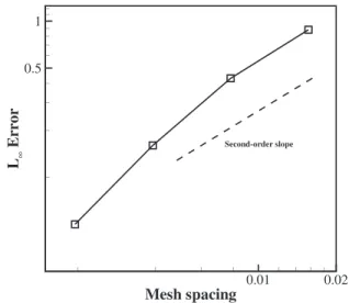
fluctuations. Here, contrary to the previous cases, 256³grid size is not enough to accurately capture the statistics. By increasing the resolution to 512³, the peak value and decay rate of enstrophy can be captured with good accuracy. This further confirms the accuracy of the present model in capturing the physics of compressible turbulence. Moreover, the convergence order of the model is evaluated based on theL1error of enstrophy with respect to the DNS results. As shown inFig. 11, the overall accuracy in space is slightly below second-order.

2. Effect of deviation discretization on the accuracy As pointed out earlier, first-order upwind discretization of the deviation term is necessary for preventing the Gibbs phenomenon and maintaining the stability of the model in supersonic regime.

FIG. 8.Time history of root mean square of dilitation for compressible decaying tur- bulence at Ma_t¼0:3 and Re_k¼72. Lines: present model; symbol: DNS.⁴²

FIG. 9.Time history of root mean square of density for compressible decaying tur- bulence at Ma_t¼0:3 and Re_k¼72. Lines: present model; symbol: DNS.⁴²

FIG. 10.Time history of enstrophy for compressible decaying turbulence at Ma_t¼0:3 and Re_k¼72. Lines: present model; symbol: DNS.⁴⁹

FIG. 11.Convergence rate of enstrophy for grid resolutions 64³to 512³. Symbols:

L1error of enstrophy with respect to the DNS results; dashed line: second-order slope.

Here, we investigate the effect of the discretization scheme on the accuracy in subsonic turbulent regime, by comparing the results to the case with the second-order central evaluation of derivatives of deviation term. It can be seen fromFig. 12that, the time history of enstrophy is insensitive to the evaluation of devia- tion term. All other turbulence statistics showed similar behavior, but are not presented here for the sake of brevity. This indicates that the use of a first-order scheme does not degrade the formal accuracy of the solver (shown inFig. 11), although it provides sufficient dissipation for stabilizing the solver and capturing the shock.

3. High turbulent Mach number

We now move on to a higher turbulent Mach number. It is well known that at sufficient high turbulent Mach numbers, random shock waves commonly known as eddy-shocklets appear in the flow,^40,42,43 due to compressibility and turbulent motions. This scenario can, therefore, be considered as a rigorous test case for the validity of the present model.

We increase the turbulent Mach number to Mat¼0:5 and per- form the simulation with 256³and 512³ grid points and the same Reynolds number Rek¼72. The iso-surface of the velocity divergence colored by local Mach number is shown inFig. 13, which confirms the presence of local supersonic regions during the decay. Moreover, to show that the model can accurately predict turbulent statistics in the presence of shocks, time evolution of the turbulent kinetic energy, rms FIG. 12.Effect of deviation discretization on the enstrophy evolution for compress-

ible decaying turbulence at Ma_t¼0:3 and Re_k¼72. Lines: present model with first-order upwind discretization of deviation term; symbols: present model with second-order central difference discretization of deviation term.

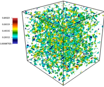
FIG. 13.Iso-surface of velocity divergence$u¼0:015, colored by local Mach number for compressible decaying turbulence at Ma_t¼0:5;Re_k¼72, and t¼0:4.

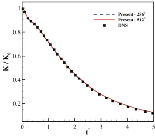
FIG. 14.Decay of the turbulent kinetic energy for compressible decaying turbulence at Ma_t¼0:5 and Re_k¼72. Lines: present model; symbol: DNS.⁴²

FIG. 15.Time history of root mean square of density for compressible decaying tur- bulence at Mat¼0:5 and Rek¼72. Lines: present model; symbol: DNS.⁴²

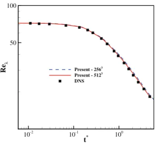
of density and Taylor microscale Reynolds number are plotted in Figs. 14–16, respectively. Here also the results agree well with the refer- ence DNS results.

As a final validation case, we investigate the performance of the model at a relatively high Reynolds number of Rek¼175, while keeping the turbulent Mach number high enough Mat¼0:488. The initial spectrum peaks atj₀¼4ð2p=LÞin this case.

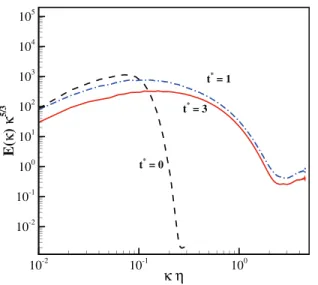
History of turbulent kinetic energy, solenoidal dissipation rate ¼ hlx²iand Taylor miroscale Reynolds number(102)are plotted inFigs. 17–19, using 768³grid points. The results agree well with the reference DNS solution.⁴²The energy spectrum at various times is shown inFig. 20. It is observed that initially, large scales contain most

of the energy and as time evolves the energy is transferred to small scales. Moreover, since the Reynolds number is high enough, the spec- trum shows the inertial range with slope ofj⁵⁼³which further con- firms the accuracy of the results and shows the ability of the model in capturing broadband turbulent motions in the presence of shocks.

IV. CONCLUSION

In this work, we proposed a lattice Boltzmann framework for the simulation of compressible flows on standard lattices. The product- form factorization was used to represent all pertinent equilibrium and quasi-equilibrium populations. The well-known anomaly of the stan- dard lattices was eliminated by redefining the diagonal components of FIG. 16.Time history of Taylor microscale Reynolds number for compressible

decaying turbulence at Mat¼0:5 and Rek¼72. Lines: present model; symbol:

DNS.⁴²

FIG. 17.Decay of the turbulent kinetic energy for compressible decaying turbulence at Mat¼0:488 and Rek¼175. Line: present model; symbol: DNS.⁴²

FIG. 18.Time history of the dissipation rate for compressible decaying turbulence at Ma_t¼0:488 and Re_k¼175. Line: present model; symbol: DNS.⁴²

FIG. 19.Time history of Taylor microscale Reynolds number for compressible decaying turbulence at Ma_t¼0:488 and Re_k¼175. Line: present model; symbol:

DNS.⁴²