Comparing methods for analysing time scale dependent
1
correlations in irregularly sampled time series data
2
Maria Reschke
a,b, Torben Kunz
a, Thomas Laepple
a 13
a Alfred Wegener Institute Helmholtz Centre for Polar and Marine Research, Telegrafenberg A45, 14473 Potsdam, 4
Germany 5
b Institute of Earth and Environmental Sciences, University of Potsdam, Karl-Liebknecht-Str. 24/25, 14476 6
Potsdam, Germany 7
Correspondence to: M. Reschke (mreschke@awi.de) 8
Abstract 9
Time series derived from paleoclimate archives are often irregularly sampled in time and thus not analysable using 10
standard statistical methods such as correlation analyses. Although measures for the similarity between time series 11
have been proposed for irregular time series, they do not account for the time scale dependency of the relationship.
12
Stochastically distributed temporal sampling irregularities act qualitatively as a low-pass filter reducing the 13
influence of fast variations from frequencies higher than about 0.5 (∆𝑡$%&)(), where ∆𝑡$%& is the maximum time 14
interval between observations. This may lead to overestimated correlations if the true correlation increases with 15
time scale. Typically, correlations are underestimated due to a non-simultaneous sampling of time series.
16
Here, we investigated different techniques to estimate time scale dependent correlations of weakly irregularly 17
sampled time series, with a particular focus on different resampling methods and filters of varying complexity.
18
The methods were tested on ensembles of synthetic time series that mimic the characteristics of Holocene marine 19
sediment temperature proxy records. We found that a linear interpolation of the irregular time series onto a regular 20
grid, followed by a simple Gaussian filter was the best approach to deal with the irregularity and account for the 21
time scale dependence. This approach had both, minimal filter artefacts, particularly on short time scales, and a 22
minimal loss of information due to filter length.
23
1 Author contributions: M.R. and T.L. designed the research, M.R. and T.K. and T.L. developed the
methodology. M.R. wrote the computer code, performed the analysis and wrote the first draft of the manuscript.
All authors contributed to the interpretation and to the preparation of the final manuscript.
Keywords: irregular sampling, time scale dependence, correlation, resampling methods 1
1 Introduction 2
Variations in past climate and environmental conditions have been recorded in many forms, including sediment 3
and ice cores, from which they can be extracted as paleoclimate time series data. Analysing these data sets provides 4
valuable insights into the drivers affecting both climate and the ecosystem on regional and global scales. One 5
obstacle that complicates the analysis of paleoclimate proxy records using standard statistical methods is the 6
temporal irregularity of the available data.
7
This patchiness and resulting temporal irregularity may have different reasons. For instance, the physical sampling 8
of the archive might be irregular due to a lack of analysable material. In the case of sedimentary archives, 9
sedimentation or accumulation rates generally vary over time, thus a regular spatial sampling of the core may lead 10
to an irregular temporal sampling of past conditions.
11
Time series data often contain several processes acting on different time scales (e.g. monthly, decadal, centennial) 12
and one approach to identify these processes is to compare different data sets and analyse their relationship at 13
different time scales. This can be achieved by estimating the coherency, although robustly determining the phase 14
and the relationship as a function of frequency requires long time series.
15
A simpler statistic that describes the similarity between two time series is the linear correlation. By definition, the 16
correlation estimate includes information about the shared variability from the Nyquist frequency (half the 17
sampling rate ∆𝑡()) to the reciprocal length of the record.
18
For many applications, a time scale dependent estimate of the correlation would be useful. For example, two time 19
series containing the same low frequency signal, but different uncorrelated (white) noise, would exhibit a higher 20
correlation if the correlation estimate was restricted to long time scales (i.e., low frequencies), because at short 21
time scales (i.e., high frequencies) the signal is largely masked by the noise (Fig. 1). Thus, it is necessary to specify 22
for which frequency range the correlation is estimated.
23
Standard routines for estimating the correlation of time series do not usually provide a possibility to make these 24
estimates frequency dependent. Furthermore, it is impossible to apply these routines directly to irregular time 25
series data. Instead, irregular data is typically resampled at a constant rate before applying the standard statistical 26
routines. However, depending on the resampling method this may bias the analysis as spectral estimates may be 27
affected by the resampling or interpolation method whose impact strongly increases with frequency (Broersen, 28
2000). Depending on the resampling frequency, this approach may add power on short time scales due to aliasing, 29
which can only be diminished by using a higher resampling frequency (Broersen, 2009). Nearest neighbour 30
interpolation results in a bias due to shifting the observation times to regular sampling (Broersen, 2009). Linear 1
interpolation causes a variance reduction toward high frequencies of the spectrum (Schulz and Stattegger, 1997).
2
Thus, interpolation acts as a low-pass filter which causes a reddening of the original signal (Schulz and Stattegger, 3
1997; Schulz and Mudelsee, 2002). This bias not only affects spectral analyses, but also time-domain methods 4
(Schulz and Statteger, 1997).
5
There are a few types of techniques (mainly developed for spectral analyses) that can be directly applied to 6
irregularly sampled data. Three approaches are shortly summarized by Broersen et al. (2000): (1) direct transform 7
methods like the Lomb-Scargle method (Lomb, 1976; Scargle, 1989), (2) slotting methods (Edelson and Krolik, 8
1988; Tummers and Passchier, 1996), and (3) model-based estimators (van Maanen and Oldenziel, 1998; Müller 9
et al., 1998). Rehfeld et al. (2011) tested these techniques for estimating the correlation of irregularly sampled time 10
series including different kernel methods in the time domain such as slotting and non-rectangular kernels. While 11
these techniques enable correlation estimates directly from irregularly sampled data, they do not consider possible 12
time scale dependencies of the correlation.
13
In this study, we investigate methods to estimate the time scale dependent correlation of weakly irregularly 14
sampled time series. As fast Fourier transform based estimators have been shown to be inferior for these kinds of 15
analyses (Rehfeld et al., 2011), we focus on methods in the time domain and two aspects in particular: (i) the time 16
scale dependency, and (ii) how best to handle the sampling irregularity.
17
While the first part focuses on finding methods that are sensitive to the time scale dependency in general, the 18
second part evaluates their applicability to irregularly sampled time series. This is accomplished through surrogate 19
time series that show the same characteristics as Holocene marine sediment temperature proxy records.
20
2 Methods 21
2.1 Time scale dependency 22
Since the correlation of time series is generally a function of time scale (i.e. the frequency range), we applied linear 23
response filters to the data in the time domain before estimating the correlation. Mathematically, the filter process 24
is defined as the convolution of an input time series with the impulse response function of the filter. In the 25
frequency domain, a filter is defined by its transfer function given by the Fourier transform of the impulse response 26
function. Commensurate with the filter effect in the time domain, the power spectrum of a filtered time series is 27
given by the product of the power spectrum of the input time series and the squared transfer function.
28
In the following, the correlation at time scale 𝑇+ is defined as the correlation obtained from the low-pass filtered 29
data with cut-off frequency 𝑓+ (= 𝑇+()). Specifically, we tested finite response filters of varying complexity: (A) 30
a moving average (boxcar) filter, common in paleoclimate research; (B) a Gaussian filter, as a compromise of a 1
short filter both in the time and frequency domains; and (C) a finite response filter with a sharp cut-off in the 2
frequency domain. The frequency response of the moving average filter depends on the filter length which we 3
defined as half of the length of the time scale for which we analysed, and the statistical filter weights were set to 4
the reciprocal filter lengths. The width parameter 𝜎 in the Gaussian filter, commonly known as the standard 5
deviation of the Gaussian function, was set to 6
𝜎 = )
012 45 (3)3 , (1)
7
which ensures that the squared transfer function of the filter decreases to 0.25 at the cut-off frequency 𝑓+. We set 8
the filter length to 6𝜎 as filter weights beyond ±3𝜎 are sufficiently close to zero and thus negligible.
9
The finite response filter consisted of the low-pass filter from Bloomfield (1976), where the weights depend on 10
both the cut-off frequency and the filter length that defines the filter sharpness. A wider time window of the filter 11
will cause the frequency response of the low-pass to converge toward a perfect cut-off filter in the frequency 12
domain. The filter length was set to five times the time scale for which we analysed. An example of all three filter 13
types is shown in Fig. 2.
14
2.2 Irregularity 15
We define an irregularly sampled time series of length 𝑁 as a sequence of observations 𝑥;(;<<)
whose observation 16
times 𝑡;(;<<)
increase monotonically with variable inter-observation time steps Δ𝑡;= 𝑡;(;<<)− 𝑡;()(;<<)
and a mean 17
sampling interval.
18
The time domain filters were applied at regular output positions 𝑡?(<@A) and different filtering procedures were 19
tested: (1) direct filtering of the irregular time series, (2) an integrand interpolation method that interpolates the 20
integrand of the convolution integral of the filter, and (3) an interpolation method that interpolates the irregular 21
time series onto a regular sampling grid before filtering. The first approach filtered and resampled the irregular 22
time series without interpolation and produced a filtered time series, 𝑥?, at the regular sampling points 𝑡?(<@A) as 23
𝑥?= B(CD
(EFG)(CH(HEE))∙&H(HEE) JHKL
B(CD(EFG)(CH(HEE)) JHKL
, (2)
24
where 𝑊(𝑡) are filter weights of our tested symmetric filters. The integrand interpolation method used the 25
procedure from Eng and Gustafsson (2008), by which the irregular time series was filtered at regular positions 26
𝑡?(<@A) and the integrand of the filter-specific convolution integral 𝐼;(;<<)
interpolated. We applied a linear 1
interpolation, yielding a filtered time series 2
𝑥?= OH(HEE)POHQL(HEE)
R ∆𝑡;
S;T) (3)
3
with the integrand of the convolution integral being 4
𝐼;(;<<)= 𝑊(𝑡?(<@A)− 𝑡;(;<<))𝑥;(;<<). (4)
5
Particularly in the geosciences, irregularly sampled time series data are commonly interpolated using linear or 6
nearest neighbour interpolations to produce a regular time series, 𝑥;(<@A) at 𝑡;(<@A), which is then filtered at the 7
regular positions 𝑡?(<@A) to yield 8
𝑥?= B(CD
(EFG)(CH(EFG))∙&H(EFG) JHKL
B(CD(EFG)(CH(EFG)) JHKL
. (5)
9
To identify the best method for estimating time scale dependent correlations between irregularly sampled time 10
series, we tested each method on surrogate time series data (with known correlations) that were modelled on 11
Holocene marine sediment temperature proxy records. We employed a Monte Carlo approach with 10 000 12
repetitions to generate pairs of irregularly sampled surrogate time series with a predefined correlation. They were 13
resampled and filtered at regular positions with a sampling interval well below the mean sampling interval, before 14
calculating the Pearson correlation with standard routines and comparing the result with the known correlations.
15
2.3 Surrogate data 16
2.3.1 Construction of surrogate signals 17
Climate signals are often dominated by low frequencies (Hasselmann, 1976). The variability in climate proxy time 18
series on interannual to multimillennial time scales can be described as a power-law process whose power spectral 19
density (PSD) is given by 𝑃𝑆𝐷 = 𝑓(X, with frequency 𝑓 and spectral slope 𝛽 (Huybers and Curry, 2006). For 20
temperature related paleoclimate signals, typical values for 𝛽 are in range of red noise between 0.3 and 1.6 21
(Huybers and Curry, 2006) with 𝛽 ≈ 1 for the Holocene (Laepple and Huybers, 2014). Due to various non-climate- 22
related factors such as a varying sedimentation rate or different sampling protocols, each proxy record contains an 23
unknown noise component (Laepple and Huybers, 2013), which, to a first degree, can be described as an 24
uncorrelated white noise, equivalent to a power-law process with 𝛽 = 0.
25
Our surrogate data was therefore constructed from pairs of annually resolved time series 𝑋 and 𝑌 of length 𝑁 = 26
10 000, each containing a superposition of a climate signal 𝑆 with a spectral slope 𝛽_ and independent random 27
noise components 𝜀& and 𝜀a with a spectral slope 𝛽b: 28
𝑋 = 𝑆 + 𝑐𝜀& (6) 1
𝑌 = 𝑆 + 𝑐𝜀a, 2
where 𝑐 is a scaling factor. All components of both time series are uncorrelated, i.e. 𝑐𝑜𝑟 𝑆, 𝜀& = 𝑐𝑜𝑟 𝑆, 𝜀a = 3
𝑐𝑜𝑟 𝜀&, 𝜀a = 0, and the associated variances 𝜎h, 𝜎bi and 𝜎bj are equal to 1.
4
The Pearson correlation of two time series is defined as their standardized covariance given by 5
𝜌lm= +no (l,m)
pq3 pr3. (7)
6
As signal and noise are uncorrelated, the covariance of 𝑋 and 𝑌 is equal to the variance of the signal component.
7
In addition, the characteristics of the noise components are identical which yields identical scaling factors. This 8
simplifies the correlation of the time series to 9
𝜌lm= ps3
ps3Ppt3+3. (8)
10
The scaling factor 𝑐 is used to scale the amplitudes of the noise components and thus to set the true correlation 11
𝜌n<;A. To get an analytical expression of 𝑐, the correlation coefficient from Eq. (8) has to be solved for the scaling 12
factor 13
𝑐 = pps3
t3(u)
vEHG− 1). (9)
14
Finally, we normalize the time series by multiplying them with 𝜌n<;A to get a unit variance.
15
Typical correlations between pairs of Holocene marine proxy records are low because the true climate signal is 16
masked by strong non-climatic noise. Laepple and Huybers (2014) obtained mean correlations of 0.18 (for Mg/Ca 17
proxy records) and 0.08 (for Uk37 proxy records) for marine sediment proxy record time series data collected less 18
than 5000 km apart and for time scales greater than 500y.
19
2.3.2 Construction of irregular sampling 20
To obtain a realistic distribution of inter-observation time steps we characterized the properties of 56 marine 21
temperature proxy time series from the Holocene dataset of Marcott et al. (2013). The inter-observation time steps 22
of each time series were normalised by their respective means. The result was found to be gamma distributed and, 23
using the method of moments, with both the shape and rate parameters equal to 2.225. The overall mean inter- 24
observation time step between samples was 108.56y.
25
To mimic the irregular sampling in our surrogate time series 𝑋 and 𝑌, we generated gamma distributed individual 1
sequences of inter-observation time steps for each time series, using the above shape and rate parameters, and 2
multiplying the result with a mean sampling interval of 100y (Fig. 3). Each observation time 𝑡;(;<<)
corresponds to 3
the sum of all previous inter-observation time steps ∆𝑡?: 𝑡;(;<<)= ;?T)∆𝑡?. The subsampling of the annually 4
sampled time series at a position 𝑡;(;<<) was accomplished by block averaging observations between (𝑡;(;<<)−∆𝑡; 2) 5
and (𝑡;(;<<)+ ∆𝑡;P)/2). We consciously chose to use averages rather than to interpolate because particularly for 6
marine data, samples often include adjacent depths or the sample distance is smaller than the typical mixing depth 7
in the sediment (Berger and Heath, 1968).
8
2.4 Evaluation of the estimation methods 9
Our methods were evaluated by comparing the correlation of our irregularly sampled surrogate time series with 10
the known true correlation using two types of targets: (i) the true time scale dependent correlation (that would be 11
obtained from a perfect filter), and (ii) the filter-specific time scale dependent correlation (to account for a non- 12
perfect frequency response of the actual filter). The true time scale dependent correlation can be determined by 13
considering 𝜌lm as a ratio of variances [cf., Eq. (8)]. To account for the time scale dependency, the variances of 14
the power-law processes of both the signal and noise components can be calculated by integrating the power 15
spectral density of the filtered power-law processes 16
𝜎R= S0QLJj𝑓(X𝐺 𝑑𝑓. (10)
17
The lower and upper boundaries of the integral are the lowest detectable frequency, i.e., the inverse time series 18
length 𝑁(), and the Nyquist frequency, respectively. For a perfect cut-off filter, 𝐺 is a step function, defined as:
19
𝐺 = 1 (𝑓 ≤ 𝑓+) and 𝐺 = 0 (𝑓 > 𝑓+). In the filter-specific case, 𝐺 is equal to the squared transfer function which is 20
the squared absolute value of the Fourier transform of the impulse response function of our tested filter (Fig. 2).
21
In this study, we solved the above integral numerically.
22
The standard deviation and bias of the deviation from the targets was used to evaluate the quality of the estimators.
23
Since the estimated time scale dependent correlation depends on the applied filter, we focussed on the bias relative 24
to the filter-specific true time scale dependent correlation. For practical reasons, we limit our analysis on time 25
scales smaller than 1000y (1/10th of the time series length). On longer time scales, the standard deviation of the 26
correlation estimates is already higher than half of the correlation estimate which is caused by a small number of 27
independent samples used for estimating the correlation.
28
3 Results 29
3.1 Correlation of red signal - white noise time series 1
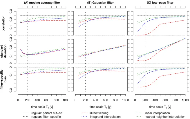
We first analyse the case consisting of a red signal (𝛽_= 1) and white noise (𝛽b= 0) with predefined correlation 2
𝜌n<;A so that the time scale dependent correlation (for time scale > 200y) is 𝜌lm= 0.1. In this case, the true time 3
scale dependent correlation increases for longer time scales (Fig. 4) as the relative influence of the noise is smaller 4
at long time scales. Since the filters do not have a perfect cut-off in the frequency domain, the filter-specific true 5
time scale dependent correlations slightly differ from the true time scale dependent correlation. While the moving 6
average filter underestimates and the Gaussian filter overestimates the correlation for all analysed time scales, the 7
low-pass filter produces correlations that are almost identical to the true time scale dependent correlation (Fig. 4).
8
All methods exhibit an increase of the correlation estimates for longer time scales similar to the true correlations 9
(Fig. 4), but differences between the estimated and the filter-specific true correlation remain.
10
On time scales shorter than 200y, all estimators overestimate the correlation, except for the direct filtering method 11
using a low-pass filter which creates a strong bias. At these shorter time scales, the integrand interpolation method 12
produced very similar results that are almost identical with the filter-specific true correlations, and only the moving 13
average overestimated the true correlation (Fig. 4).
14
On longer time scales, the estimated correlations generally converge to the filter-specific true correlation as 15
indicated by the decreasing absolute bias as the time scales are increased (Fig. 4), with the exception of the low- 16
pass filter and the direct filtering approach which both maintain a negative bias.
17
In general, the standard deviations of the estimators, describing the uncertainty of estimating the correlation from 18
a pair of finite time series, are higher than the filter-specific biases. Due to the higher uncertainties of estimating 19
the correlation on long time scales from short datasets, the standard deviations increase for longer time scales.
20
With the exception of the moving average method on short time scales, all methods exhibit higher standard 21
deviations and biases when interpolating compared to the direct filtering and integrand interpolation approach.
22
The different uncertainties are mainly due to different filter lengths. In general, longer filters have higher standard 23
deviations and lower filter-specific biases (except for parts of the low-pass based procedures) than short filters.
24
3.2 Correlation of white signal - white noise time series 25
To further investigate the properties of the estimators, we analyse the superposition of two white noise signals 26
(𝛽_= 𝛽b = 0) with a predefined correlation 𝜌n<;A= 0.25. There is no predominance of one component at any 27
frequency, so that the true correlation is time scale independent, which also holds for the filter-specific true 28
correlations (Fig. 5). For all tested methods, the estimated correlations exhibit a negative bias that appears 29
independent of both the procedure that handles the irregularity and the time domain filters used. The mismatch 1
was high for short time scales and vice versa (Fig. 5).
2
The interpolation approach, and in particular the linear interpolation vis-à-vis the nearest-neighbour, yielded the 3
best approximation of the true correlation.
4
On long time scales, the estimated correlations of the interpolation and the integrand interpolation procedure are 5
similar (except for the moving average filter), while on short time scales the integrand interpolation method 6
underestimates the filter-specific true correlation (Fig. 5). This behaviour stands in direct contrast to the results 7
obtained for the red signal and white noise (see above).
8
With regard to the uncertainties in agreement with the results from the red signal with white noise, the standard 9
deviations typically increased for longer time scales in all tested methods except the moving average filter on short 10
time scales using the direct filtering and integrand interpolation approach.
11
The standard deviation of an estimator tends to be larger than the filter-specific bias. With longer filters and for 12
long time scales, the bias was typically lower while those values were nearly equal for short time scales. The 13
observed high absolute bias of the integrand interpolation method for short time scales stands in direct contrast to 14
the low bias observed for the red signal plus white noise scenario.
15
4 Discussion 16
We focussed on three particular aspects: (1) how does temporal irregularity in sampling affect the time scale 17
dependency of correlations, (2) what is the best procedure to handle this irregularity, and (3) which is the best filter 18
to account for the time scale dependence of the correlation. We tested three different approaches to find 19
correlations in irregularly sampled time series data, namely: (i) direct filtering of irregular time series, (ii) an 20
integrand interpolation method that interpolates the integrand of the convolution integral of the filter, and (iii) an 21
interpolation that interpolates the irregular time series onto a regular sampling grid before filtering. The approaches 22
were combined with three finite response filters: (A) a moving average (boxcar) filter, (B) a Gaussian filter, and 23
(C) a finite response filter with a sharp cut-off in the frequency domain. While all tested approaches yielded similar 24
results, there were some notable differences.
25
4.1 Effect of irregularity and non-simultaneousness in sampling 26
The irregularity of the sampling affects the correlation estimate in two ways: (i) they shift the correlation toward 27
estimates related to longer time scales due to different inter-observation time steps; and (ii) the non-simultaneous 28
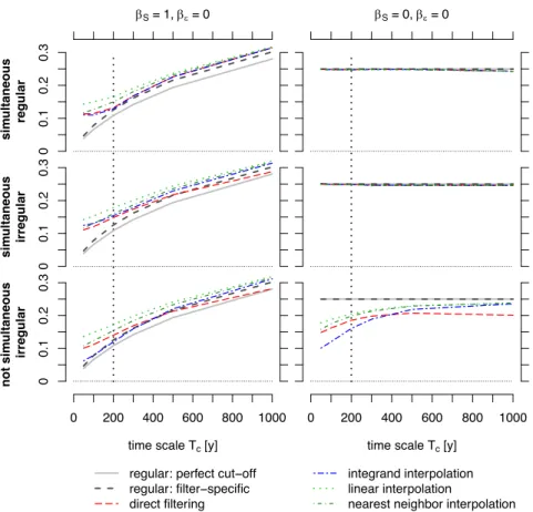
sampling of time series introduces a general bias that leads to an underestimation of the true correlation. Fig. 6 29
illustrates these effects in case of a time scale dependent (𝛽_= 1, 𝛽b= 0) as well as a time scale independent 1
(𝛽_= 0, 𝛽b= 0) correlation.
2
The sampling rate, ∆𝑡(), of a time series acts qualitatively as a first low-pass filter with a smoothed cut-off. Since 3
it is necessary to have at least two observations per detectable oscillation, the sampling-related cut-off (i.e., 4
Nyquist) frequency is 𝑓Sa= 0.5∆𝑡(). To analyse the time scale dependency of the correlation, we filtered the time 5
series a second time to remove information about oscillations smaller than the considered time scale. If the first 6
filtering process has a smaller cut-off frequency than the second one, there is an additional loss of information at 7
frequencies > 𝑓Sa (Fig. 6, top left). In the presence of a red signal, the time scale dependent correlation of a pair 8
of time series would thus be overestimated while a white noise signal would exhibit the expected time scale 9
independency of the correlation (Fig. 6, top right).
10
For two time series that were sampled at irregular intervals but simultaneous times, the short time scale correlation 11
estimates are shifted toward those for longer time scales, which is a direct result of the irregular sampling intervals 12
and the sampling-related cut-off becomes roughly 𝑓Sa= 0.5(∆𝑡$%&)(). Therefore, the shift only affects time 13
scales < 2∆𝑡$%&. If 𝑓+ > 𝑓Sa, the correlation is overestimated for red signals while remaining unchanged for white 14
noise (Fig. 6, middle row).
15
Sampling two irregular time series at non-simultaneous times removes information at different time scales and 16
different time windows from each data set. The correlation estimate of such time series is affected by both the shift 17
of short time scale related correlations toward the estimate at a time scale of 2∆𝑡$%& and an underestimation that 18
affects all time scales. White data sets are only affected by the non-simultaneity in sampling. The shift of short 19
time scale related correlations toward those observed for longer time scales we did not observe as the correlation 20
of a white noise signal is time scale independent (Fig. 6, bottom right). Both effects are seen for the data set 21
containing the red signal (Fig. 6, bottom left). In this case, the good approximation of the estimated correlation of 22
the integrand interpolation on the filter-specific true correlation is an artefact which is caused by the error- 23
proneness of the method in application on time series with a low resolution and non-simultaneous sampling.
24
4.2 Choosing the best method 25
A procedure that should handle irregularity and account for time scale dependencies must above all be robust and 26
reliable.
27
4.2.1 Handling irregularity 28
If ∆𝑡$%& exceeds the applied filter length, the filter integral becomes unreliable and the fewer observations we 29
have within the filter range the higher the associated error. Direct filtering is similar to the numerical solution of 30
the filter integral for a high resolution regularly sampled time series which is equal to the sum of the products of 1
the filter weights with their corresponding observations. Due to the irregular sampling combined with a low mean 2
sampling rate, there are only a few observations left which are used for the sum. There is thus a systematic error, 3
caused by the application of this procedure on irregularly sampled time series. This error affects all time scales, 4
but especially shorter ones. This effect was clearly visible with time series pairs whose correlation was time scale 5
independent (Fig. 5).
6
The filter integrand interpolation procedure commonly reduces the errors caused by direct filtering, because it also 7
works directly on the irregularly sampled time series, but uses additional interpolated values during the summation 8
of the products of the filter weights with their corresponding observations. Again, a higher number of observations 9
per filter window reduces the systematic error of this approach because of less over- or underestimated interpolated 10
values of the filter integral. Hence, the error is lower on longer time scales. On short time scales, there is a high 11
bias despite filter integrand interpolation (Fig. 5).
12
4.2.2 Accounting for time scale dependency 13
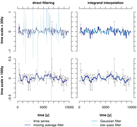
The applied filters cause artefacts based to their length as well as their cut-off behaviour. For ∆𝑡 greater than the 14
applied filter length, gaps occurred in the filtered result. According to the filter weights, which are related to the 15
cut-off behaviour of the applied filter, there were artefacts like overshooting and steps within the filtering results 16
(Fig. 7).
17
The moving average filter had the shortest length of all tested filters. There were less observations within the filter 18
window so that the standard deviation of the estimated time scale dependent correlations was lower than for the 19
other filters (Fig. 4). Higher standard deviations on short time scales which are related to the direct filtering and 20
integrand interpolation procedures are the result of gaps within the filtering results. These gaps occur if the filter 21
length is shorter than the inter-observation time steps. Especially on short time scales, this happened frequently 22
(Fig. 7, top). Since the weights of the moving average filter were equal, the filtering result appeared step-like. This 23
is independent of the analysed time scale (Fig. 7).
24
The low-pass filter was the longest tested filter and contained positive and negative filter weights. Both properties 25
can lead to artefacts. The underestimation of the correlation related to longer time scales might be the consequence 26
of the long filter length as well as the finite length of the time series itself. Especially short time series would suffer 27
from a significant loss of information due to filtering with low cut-off frequencies, so that the filtered time series 28
would be much shorter than the original data (Fig. 7, bottom left).
29
In addition, this caused a high standard deviation of the correlations for the low-pass filter. On short time scales, 30
the low correlation estimates related to the direct filtering and integrand interpolation procedures resulted from 31
filter artefacts (overshooting) due to less observations as well as positive and negative filter weights. Especially in 1
parts of the time series where the inter-observation time steps were larger than the mean sampling interval, the 2
filtered time series was affected by overshooting (Fig. 7, top left). The overshooting can be reduced by increasing 3
the number of observations per filter window or through a more regular sampling.
4
The Gaussian filter had nearly the same characteristics as the low-pass filter from Bloomfield (1976) with a filter 5
length of one-time the analysed time scale because both filters only contain positive filter weights. Therefore, here 6
the main artefact of the low-pass filter – the overshooting which is caused by negative filter weights – was limited 7
or non-existent (Fig. 7, top right). Sometimes, slight overshooting (not shown) was possible on short time scales 8
when ∆𝑡 was close to the Gaussian filter length.
9
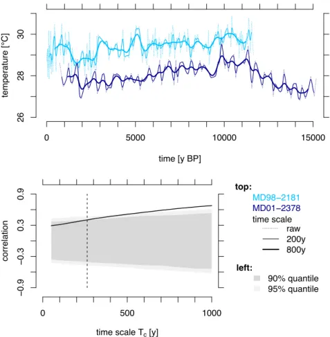
4.3 Example application to observed proxy records 10
As a final example, we applied one combination of our tested procedures and filters to data from two marine 11
sediment cores which consisted of sea surface temperature records, based on Mg/Ca measured in planktonic 12
foraminifera (Nürnberg et al., 1996). The Morotai Basin core MD98-2181 (Stott et al., 2007), located in the 13
westernmost Pacific Ocean (6.3°N, 125.8°E), and the Timor Sea core MD01-2378 (Xu et al., 2008), located in the 14
easternmost Indian Ocean (13.1°S, 121.8°E), were collected 2190 km apart, have a high mean resolution (MD98- 15
2181: 50y, MD01-2378: 130y) and overlap in time between 730 and 11 660y BP (Fig. 8).
16
We use the combination of a linear interpolation followed by Gaussian filtering to estimate the correlation related 17
to different time scales, as this method produced the fewest artefacts. To test the statistical significance of the 18
correlation estimates, we compared the estimates against the null hypothesis of uncorrelated time series with a 19
noise with power-law scaling with 𝛽 = 1 (Appendix A).
20
The correlation of the time series pair increased for longer time scales. Given the relatively high noise level in 21
Mg/Ca records (Laepple and Huybers, 2013), this suggests that the common (climate) signal is masked on short 22
time scales. Filtering the time series led to a greater reduction in the noise component compared to the common 23
climate component and resulted in statistically significant correlation estimates (p=0.05) for time scales >500y 24
(Fig. 8).
25
5 Conclusion 26
In this study, we investigated different methods to estimate the time scale dependent correlation of weakly 27
irregularly sampled time series. Each method was restricted to the time domain and overcame the sampling 28
irregularities by interpolation or direct filtering. Each method also had to account for the time scale dependency 29
of the correlation which was achieved through filtering. As data sets we used surrogate time series that mimicked 1
the characteristics of Holocene marine sediment temperature proxy records.
2
The irregularity in sampling causes problems during the correlation analyses as it qualitatively acts as a low-pass 3
filter with a cut-off frequency of roughly 0.5(∆𝑡$%&)(). Thus, estimates for time scales < 2∆𝑡$%& exhibited a bias 4
in addition to a time scale independent underestimation of the correlation which we attributed to the non- 5
simultaneous sampling of time series.
6
Both the linear and nearest neighbour interpolations were the best performers in terms of handling the sampling 7
irregularity and neither was prone to artefacts which occur if some ∆𝑡 are much larger than the mean sampling 8
interval. Although the bias and the standard deviation were both higher for the interpolation method than for the 9
integrand interpolation, we suggest the application of the interpolation method due to more reliable estimates as 10
the integrand interpolation method failed on short time scales due to the existence of artefacts.
11
The tested low-pass filter with a length five times the analysed time scale provided the best approximation to the 12
analytical solution for a perfect cut-off filter. However, the filtering result was affected by artefacts due to the long 13
filter length as well as negative filter weights. Both aspects limit the applicability of this filter.
14
The Gaussian filter was a compromise between the low standard deviation of the moving average filter and the 15
cut-off behaviour of the low-pass filter. The cut-off behaviour and filter weights were comparable to the properties 16
of a shorter version of the low-pass filter of the same definition, but with a length of one-time the analysed time 17
scale. By reason of a smoother filtering result without gaps (moving average filter) and overshooting (low-pass 18
filter), we suggest the application of the Gaussian filter.
19
Irrespective of the applied method and filter, there was the tendency for most artefacts to occur when analysing 20
short time scales if there were less observations due to a low mean sampling rate. Therefore, it is meaningful to 21
restrict the estimation of the time scale dependent correlation to time scales which are obviously larger than the 22
mean inter-observation time step of the analysed time series.
23
Appendix A: Significance test for time scale dependent correlation estimates 24
To test the significance of the time scale dependent correlation estimates, we resort to a Monte Carlo procedure.
25
We generate surrogate records on an annual scale, subsample the records at the same resolution as the analysed 26
time series and then apply our estimators. Finally, we provide the 90% and 95% quantiles of the correlations 27
obtained from the surrogate data.
28
As null-hypothesis we assume uncorrelated time series, thus time series that only consist of noise. The statistical 1
significance will depend on the temporal correlation of the noise, i.e., its power spectrum. Let us assume a power- 2
law spectrum, either with a prescribed slope, or with a slope estimated from the datasets to be tested.
3
For the latter, we estimate the spectral slopes of our time series by linearly interpolating the time series onto an 4
equidistant grid and estimating the power spectrum from the detrended time series. Finally, we estimate the slope 5
from the power spectrum by a linear regression in the frequency range of the reciprocal half of the length of the 6
overlapping time window of the time series as well as the inverse twofold maximum mean resolution of both time 7
series. Our choice of the frequency range minimized the impact of the detrending as well as the impact of the 8
irregular sampling and the linear interpolation. However, especially for short time series, the estimates of spectral 9
slopes are very uncertain.
10
For Holocene sea surface temperature paleoclimate time series, we suggest to prescribe a spectral slope of 1 11
(Laepple and Huybers, 2014) as this estimate is based on analysing a large number of sediment records and thus 12
more robust than noisy estimates based on single time series.
13
Acknowledgement 14
We would like to acknowledge Jürgen Kurths, Kira Rehfeld, Andrew Dolman, and Igor Kröner for fruitful 15
discussions. This study was supported by the Initiative and Networking Fund of the Helmholtz Association Grant 16
VG-NH900 as well as the European Research Council (ERC) under the European Union’s Horizon 2020 research 17
and innovation program (grant agreement no. 716092).
18
Computer code availability 19
The code used in this paper is based on R (³ 3.2.2). It can be downloaded as the R package ‘corit’ from the public 20
git repository at https://github.com/EarthSystemDiagnostics/corit. The main functions allow a time scale 21
dependent estimation of the Pearson correlation based on three methods resampling irregular data to an equidistant 22
spacing before or during filtering the time series, a significance test of the estimate based on surrogate records as 23
well as an output of the filtered time series. All main functions are provided with a simple example in the R 24
Documentation.
25
References 26
Berger, W. H., and Heath, G. R., 1968. Vertical mixing in pelagic sediments. Journal of Marine Research, 26, 134- 27
143.
28
Bloomfield, P., 1976. Fourier Analysis of Time Series: An Introduction. John Wiley, New York.
1
Broersen, P. M., 2009. Five Separate Bias Contributions in Time Series Models for Equidistantly Resampled 2
Irregular Data. IEEE Transactions on Instrumentation Measurement, 58(5), 1370-1379.
3
Broersen, P. M. T., de Waele, S., and Bos, R., 2000. The Accuracy of Time Series Analysis for Laser-Doppler 4
Velocimetry. In: Proceedings of the 10th International Symposium on Applications of Laser Techniques to Fluid 5
Dynamics, Lisbon, Portugal.
6
Came, R. E., Oppo, D. W., and McManus, J. F., 2007. Amplitude and timing of temperature and salinity variability 7
in the subpolar North Atlantic over the past 10 k.y., Geology, 35(4), 315-318, doi:10.1130/G23455A.1.
8
Edelson, R. A., and Krolik, J. H., 1988. The discrete correlation function - A new method for analyzing unevenly 9
sampled variability data. The Astrophysical Journal, 333, 646-659.
10
Eng, F., and Gustafsson, F., 2008. Downsampling Non-Uniformly Sampled Data. EURASIP Journal on Advances 11
in Signal Processing, doi:10.1155/2008/147407.
12
Hasselmann, K., 1976. Stochastic climate models Part I. Theory, Tellus, 28(6), 473-485.
13
Huybers, P., and Curry, W., 2006. Links between annual, Milankovitch and continuum temperature variability.
14
Nature, 441(7091), 329-332, doi:10.1038/nature04745.
15
Kubota, Y., Kimoto, K., Tada, R., Oda, H., Yokoyama, Y., and Matsuzaki, H., 2010. Variations of East Asian 16
summer monsoon since the last deglaciation based on Mg/Ca and oxygen isotope of planktic foraminifera in the 17
northern East China Sea. Paleooceanography, 25, PA4205, doi:10.1029/2009PA001891.
18
Laepple, T., and Huybers, P., 2013. Reconciling discrepancies between Uk37 and Mg/Ca reconstructions of 19
Holocene marine temperature variability. Earth and Planetary Science Letters, 375, 418-429.
20
Laepple, T., and Huybers, P., 2014. Ocean surface temperature variability: Large model–data differences at 21
decadal and longer periods. Proceedings of the National Academy of Sciences, 111(47), 16682-16687, 22
doi:10.1073/pnas.1412077111.
23
Lomb, N. R., 1976. Least-squares frequency analysis of unequally spaced data. Astrophysics and Space Science, 24
39(2), 447-462.
25
Marcott, S. A., Shakun, J. D., Clark, P. U., and Mix, A. C., 2013. A Reconstruction of Regional and Global 26
Temperature for the Past 11,300 Years. Science, 339(6124), 1198-1201, doi:10.1126/science.1228026.
27
Müller, E., Nobach, H., and Tropea, C., 1998. Model parameter estimation from non-equidistant sampled data sets 28
at low data rates. Measurement Science Technology, 9(3), 435-441.
29
Nürnberg, D., Bijma, J., and Hemleben, C., 1996. Assessing the reliability of magnesium in foraminiferal calcite 30
as a proxy for water mass temperatures. Geochimica et Cosmochimica Acta, 60(5), 803-814.
31
Rehfeld, K., Marwan, N., Heitzig, J., and Kurths, J., 2011. Comparison of correlation analysis techniques for 1
irregularly sampled time series. Nonlinear Processes in Geophysics, 18(3), 389-404, doi:10.5194/npg-18-389- 2
2011.
3
Scargle, J. D., 1989. Studies in astronomical time series analysis. III - Fourier transforms, autocorrelation 4
functions, and cross-correlation functions of unevenly spaced data. The Astrophysical Journal, 343, 874-887.
5
Schulz, M., and Mudelsee, M., 2002. REDFIT: estimating red-noise spectra directly from unevenly spaced 6
paleoclimatic time series. Computers & Geosciences, 28(3), 421-426.
7
Schulz, M., and Stattegger, K., 1997. SPECTRUM: Spectral analysis of unevenly spaced paleoclimatic time series.
8
Computers & Geosciences, 23(9), 929-945.
9
Stott, L., Timmermann, A., and Thunell, R., 2007. Southern Hemisphere and Deep-Sea Warming Led Deglacial 10
Atmospheric CO2 Rise and Tropical Warming. Science, 318(5849), 435-438, doi:10.1126/science.1143791.
11
Tummers, M. J., and Passchier, D. M., 1996. Spectral estimation using a variable window and the slotting 12
technique with local normalization. Measurement Science and Technology, 7(11), 1541-1546.
13
van Maanen, H. R. E., and Oldenziel, A., 1998. Estimation of turbulence power spectra from randomly sampled 14
data by curve-fit to the autocorrelation function applied to laser-Doppler anemometry. Measurement Science and 15
Technology, 9(3), 458-467.
16
Xu, J., Holbourn, A., Kuhnt, W., Jian, Z., and Kawamura, H., 2008. Changes in the thermocline structure of the 17
Indonesian outflow during Terminations I and II. Earth and Planetary Science Letters, 273(1), 152-162.
18
1
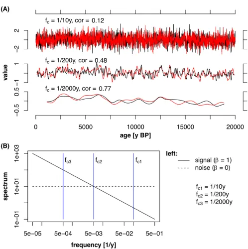
Figure 1: Time scale dependent correlation of an irregularly sampled time series pair (A) and spectrum of 2
the signal and white noise (B). The time series 1 and 2 (red and black) contain the same signal, generated as red 3
noise with 𝛽_= 1 and independent white noise components. Both time series are filtered with three cut-off 4
frequencies 𝑓+ and the resulting time series are shown (A). The time series containing most frequencies (𝑓+ = 1/10y) 5
is basically uncorrelated while slow variations are positively correlated as seen after filtering with 𝑓+ = 1/2000y.
6
This can be also understood in the spectral domain (B). The power spectral density of the signal (solid black line) 7
increases towards lower frequencies whereas the power spectral density of the noise (dashed black line) is constant.
8
For high cut-off frequencies such as 𝑓+ = 1/10y the variance of the noise is higher than the variance of the signal 9
as given by the integrated spectra of the signal and the noise up to 𝑓+ (area between axes, 𝑓+ and the power spectral 10
density). For decreased 𝑓+ the integrated spectrum of the signal becomes more dominant relative to the noise. The 11
higher amount of the signal compared to the noise component results in higher correlations for time series filtered 12
with lower 𝑓+. 13
−22
value
fc = 1/10y, cor = 0.12
−11 fc = 1/200y, cor = 0.48
0 5000 10000 15000 20000
fc = 1/2000y, cor = 0.77
age [y BP]
−0.50.5
5e−05 5e−04 5e−03 5e−02 5e−01
1e−011e+011e+03
frequency [1/y]
spectrum
left:
fc1
fc2
fc3 signal (b = 1)
noise (b = 0)
fc1 = 1/10y fc2 = 1/200y fc3 = 1/2000y (A)
(B)
1
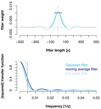
Figure 2: Characteristics of the filters used in this study. Upper panel: Filter weights in the time domain. Lower 2
panel: Squared transfer function in the frequency domain with marked cut-off frequency (dashed line). The low- 3
pass filter is characterized by a sharp cut-off in the frequency domain, the moving average by its short length in 4
the time domain. The Gaussian filter has the same simple shape in the time and the frequency domain. These 5
examples are for a time scale of 200y.
6
−500 −300 −100 100 300 500 filter length [y]
−0.0050.0050.015
filter weight
0 0.01 0.02 0.03 0.04 0.05
frequency [1/y]
00.40.8
[squared] transfer function
Gaussian filter moving average filter low−pass filter
1
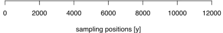
Figure 3: Examples of sampling irregularity. The sampling times of two typical marine sediment cores KY07- 2
04-01 (Kubota et al., 2010) and ODP 984 (Came et al., 2007) are shown in the upper two rows. The lower two 3
rows show examples of surrogate sampling times generated using gamma-distributed inter-observation time steps 4
as described in the Method section.
5
Irregularity in Sampling
0 2000 4000 6000 8000 10000 12000
sampling positions [y]
ODP 984 KY07−04−01
Surrogate 1 Surrogate 2
● ● ●●●●●●●●●● ●● ● ●●●●●●● ●●● ● ● ● ● ● ● ● ●●● ● ● ● ● ●●●●● ● ● ● ● ● ●●●●● ● ● ● ● ● ● ● ● ●●●●●● ●●● ● ● ● ●● ● ● ● ● ● ● ●● ● ● ● ● ● ● ● ●● ● ●● ● ●● ● ● ● ● ●● ● ● ● ●●● ● ● ● ●●
●●● ●●●● ●●●●●● ●● ● ● ● ●● ● ● ● ● ●●● ● ●●● ●● ● ●● ● ● ●● ●● ● ● ● ● ● ● ●● ● ● ●● ● ● ●● ● ● ●● ● ● ● ● ●●● ● ●● ● ● ● ● ● ● ● ●● ● ● ● ● ● ● ● ●●● ●●● ●
●
● ● ● ●● ●●●●●●● ● ●● ● ●● ● ● ● ●●● ●● ● ● ●● ● ● ●● ●●●●●●●● ●●●●●●● ●● ●● ● ● ●●● ●●●●●●● ● ●● ●● ●●●●●● ● ● ● ●●● ●●●● ●●●● ●●● ●● ● ● ●
● ●●● ●● ● ●● ● ●● ● ●●●●●● ●●●● ●● ●●●● ● ● ●● ●● ●● ●●●● ●● ●● ● ●● ●●●● ●● ● ●● ●● ● ● ●●● ● ●● ●● ● ● ● ●●● ● ●●●●●●●●● ●●● ● ●● ●●●●●●●● ●
1
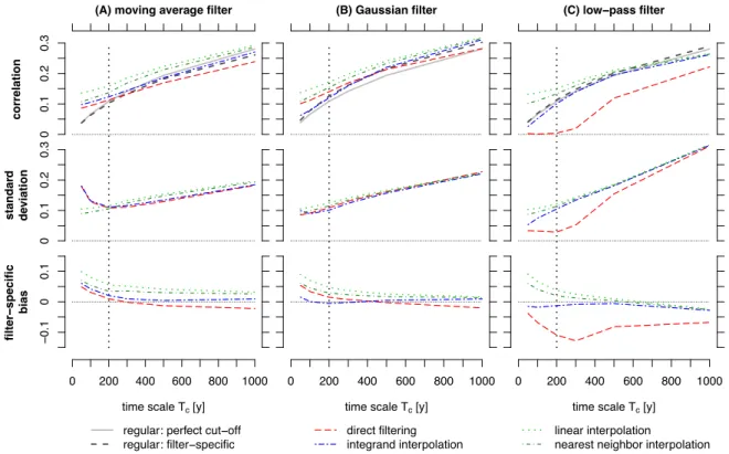
Figure 4: Performance of the different estimation methods for a red signal (𝜷𝑺= 𝟏) with white noise 2
component (𝜷𝜺= 𝟎). Top row: True correlation (grey, black) and estimated correlation (colours) as a function of 3
time scale. Middle row: Standard deviation of the estimators. Bottom row: Bias of the estimators relative to the 4
filter-specific true correlation. The dashed vertical line marks the time scale corresponding to the mean sampling 5
interval.
6
0 200 400 600 800 1000
time scale Tc [y]
00.10.20.3
correlation 00.10.20.3
standard deviation −0.100.1
filter−specific bias
(A) moving average filter
regular: perfect cut−off regular: filter−specific
0 200 400 600 800 1000
time scale Tc [y]
(B) Gaussian filter
direct filtering integrand interpolation
0 200 400 600 800 1000
time scale Tc [y]
(C) low−pass filter
linear interpolation
nearest neighbor interpolation
1
Figure 5: Performance of the different estimation methods for a white noise signal (𝜷𝑺= 𝟎) with white noise 2
component (𝜷𝜺= 𝟎). Top row: True correlation (grey, black) and estimated correlation (colours) as a function of 3
time scale. Middle row: Standard deviation of the estimators. Bottom row: Bias of the estimators relative to the 4
filter-specific true correlation. Vertical dashed lines mark the time scale corresponding to the mean sampling 5
interval. As the spectrum of the white noise signal and noise is constant, the true correlation is time scale 6
independent.
7
0 200 400 600 800 1000
time scale Tc [y]
00.10.20.3
correlation 00.10.20.3
standard deviation −0.3−0.10
filter−specific bias
(A) moving average filter
regular: perfect cut−off regular: filter−specific
0 200 400 600 800 1000
time scale Tc [y]
(B) Gaussian filter
direct filtering integrand interpolation
0 200 400 600 800 1000
time scale Tc [y]
(C) low−pass filter
linear interpolation
nearest neighbor interpolation
1
Figure 6: Effect of irregular and non-simultaneous sampling on the correlation estimates. Correlations are 2
estimated by applying a Gaussian filter on regularly (top), irregularly but simultaneously (mid), and irregularly 3
but non-simultaneously (bottom) sampled time series as a superposition of a red signal and white noise (left), and 4
white noise signal and white noise (right). The vertical dashed lines mark the time scale corresponding to the mean 5
sampling interval. The simultaneous, irregular sampling is affected by a shift of the correlation estimates toward 6
longer time scales, which is not visible in case of the white signal and noise (right). Sampling that is irregular but 7
non-simultaneous will underestimate the correlation.
8
0 200 400 600 800 1000
time scale Tc [y]
00.10.20.3
simultaneous regular 00.10.20.3
simultaneous irregular 00.10.20.3
not simultaneous irregular
bS = 1, be = 0
regular: perfect cut−off regular: filter−specific direct filtering
0 200 400 600 800 1000
time scale Tc [y]
bS = 0, be = 0
integrand interpolation linear interpolation
nearest neighbor interpolation