The Expedition PS115/1
of the Research Vessel POLARSTERN to Greenland Sea and Wandel Sea in 2018
Edited by
Volkmar Damm
with contributions of the participants
Berichte
zur Polar- und Meeresforschung
Reports on Polar and Marine Research
727
2019
Die Berichte zur Polar- und Meeresforschung ent- halten Darstellungen und Ergebnisse der vom AWI selbst oder mit seiner Unterstützung durchgeführten Forschungsarbeiten in den Polargebieten und in den Meeren.
Die Publikationen umfassen Expeditionsberichte der vom AWI betriebenen Schiffe, Flugzeuge und Statio- nen, Forschungsergebnisse (inkl. Dissertationen) des Instituts und des Archivs für deutsche Polarforschung, sowie Abstracts und Proceedings von nationalen und internationalen Tagungen und Workshops des AWI.
Die Beiträge geben nicht notwendigerweise die Auf- fassung des AWI wider.
The Reports on Polar and Marine Research contain presentations and results of research activities in polar regions and in the seas either carried out by the AWI or with its support.
Publications comprise expedition reports of the ships, aircrafts, and stations operated by the AWI, research results (incl. dissertations) of the Institute and the Archiv für deutsche Polarforschung, as well as abstracts and proceedings of national and international conferences and workshops of the AWI.
The papers contained in the Reports do not necessarily reflect the opinion of the AWI.
Herausgeber
Dr. Horst Bornemann
Redaktionelle Bearbeitung und Layout Birgit Reimann
Editor
Dr. Horst Bornemann Editorial editing and layout Birgit Reimann
Alfred-Wegener-Institut
Helmholtz-Zentrum für Polar- und Meeresforschung Am Handelshafen 12
27570 Bremerhaven Germany
www.awi.de www.reports.awi.de
Titel: Das 3.000 m lange seismische Streamerkabel wird zu Wasser gelassen (Foto: Dr. Thomas Funck/GEUS Kopenhagen)
Cover: Deploying the 3,000 m long seismic streamer cable (Photo: Dr. Thomas Funck/GEUS Copenhagen)
Alfred-Wegener-Institut
Helmholtz-Zentrum für Polar- und Meeresforschung Am Handelshafen 12
27570 Bremerhaven Germany
www.awi.de www.reports.awi.de
Der Erstautor bzw. herausgebende Autor eines Ban- des der Berichte zur Polar- und Meeresforschung versichert, dass er über alle Rechte am Werk verfügt und überträgt sämtliche Rechte auch im Namen sei- ner Koautoren an das AWI. Ein einfaches Nutzungs- recht verbleibt, wenn nicht anders angegeben, beim Autor (bei den Autoren). Das AWI beansprucht die Publikation der eingereichten Manuskripte über sein Repositorium ePIC (electronic Publication Information Center, s. Innenseite am Rückdeckel) mit optionalem print-on-demand.
The first or editing author of an issue of Reports on Polar and Marine Research ensures that he possesses all rights of the opus, and transfers all rights to the AWI, including those associated with the co-authors. The non-exclusive right of use (einfaches Nutzungsrecht) remains with the author unless stated otherwise.
The AWI reserves the right to publish the submitted articles in its repository ePIC (electronic Publication Information Center, see inside page of verso) with the option to "print-on-demand".
Please cite or link this publication using the identifiers
http://hdl.handle.net/10013/epic.886c25f8-fdba-42b1-aad3-4e2f53c81a65 and https://doi.org/10.2312/BzPM_0727_2019
The Expedition PS115/1
of the Research Vessel POLARSTERN
to the Greenland Sea and Wandel Sea in 2018
Edited by
Volkmar Damm
with contributions of the participants
5 August 2018 - 3 September 2018 Tromsø - Longyearbyen
Chief scientist Volkmar Damm
Coordinator
Rainer Knust
1. Überblick und Fahrtverlauf 3
Summary and itinerary 4
2. Weather Conditions 11
3. Structural Investigations off North East and North Greenland
Based on Geophysical Data 14
3.1 Reflection seismic data acquisition 15
3.2 Wide angle seismic data using sonobuoys 25
3.3 Refraction seismic data (OBS) 28
3.4 Magnetics 34
3.5 Gravity 41
3.6 Heatflow density measurements 52
4. Geological Sampling for Thermochronological Studies 61 5. Microbiological and Geochemical Investigations to Understand
Gases and Microbial Processes in Arctic Seafloor Sediments 68
5.1 Geomicrobiology 68
5.2 Sediment and pore water geochemistry 72
6. Sediment Coring for Reconstruction of the Environmental and
Climate History off NE Greenland (ECHONEG) 75 7. Bathymetric Mapping and Sub-bottom Profiling 79
7.1 Bathymetric mapping 79
7.2 Sub-bottom profiling 82
8. At Sea Distribution of Sea Birds and Marine Mammals 84 9. The “Year of Polar Prediction” (Yopp):
Additional Radio-Soundings during the Special Observing Period 88 10. Mitigation Measures during Seismic Operations 90
10.1 Standard MMO and PAM operations and
service provided by SML 91
10.2 Automatic Infrared-based Marine Mammal Mitigation
System (AIMMMS) 118
11. Outreach – Documentation of PS115/1 124
Appendix
A.1 Teilnehmende Institute / Participating Institutions 126
A.2 Fahrtteilnehmer / Cruise Participants 128
A.3 Schiffsbesatzung / Ship's Crew 130
A.4 Stationsliste / Station List 131
A.5 List of Sediment Cores 145
A.6 MMO of Weekly Reports 173
Volkmar Damm BGR
Die Expedition PS115/1 startete am 5. August 2018 in Tromsø (Norwegen) und endete am 3.
September 2018 in Longyearbyen (Spitzbergen; s. Abb. 1.1).
Mit dieser Reise von Polarstern wurden im Rahmen des BGR-Projekts GREENMATE multidisziplinäre geowissenschaftliche Forschungsarbeiten durchgeführt, die zu einem besseren Verständnis der geologischen Entwicklung des Europäischen Nordmeeres und der Schelfgebiete Nordost- und Nordgrönlands führen sollen. Den Schwerpunkt bildeten einerseits marine geophysikalische Untersuchungen mittels seismischer, magnetischer, gravimetrischer und geothermischer Verfahren und andererseits geologische Beprobungsarbeiten unter Einsatz von Schwerelot, Kastengreifer, Multicorer und Dredge. Die Arbeiten zur Beprobung mariner Schelfsedimente wurden in enger Abstimmung mit der Nebennutzergruppe des GEOMAR geplant und durchgeführt. Das Probenmaterial ist Grundlage für die geplanten Arbeiten zur Rekonstruktion der Paläoumwelt- und Paläoklimaentwicklung der jüngeren geologischen Geschichte im Rahmen des Projekts ECHONEG (s. Kapitel 6).
Unter Nutzung der bordeigenen Helikopter wurden die marinen Beprobungen durch geologische Probenahmen an einzelnen küstennahen Lokationen ergänzt.
Weitere wissenschaftliche Projektgruppen nutzten die Reise PS115/1 zur Erfassung mariner Säuger und Seevögel entlang der Fahrtstrecke, um zu Daten über deren statistische Verteilung im Fahrtgebiet als Teilbeitrag für ein langfristig angelegtes Beobachtungsprogramm (Projekt Birds & Mammals – Kapitel 8) zu gelangen, und im Rahmen eines weiteren Langzeitbeobachtungsprogramms zur Erhebung meteorologischer Daten mittels zusätzlicher Radiosondenaufstiege (Projekt YOPP – Kapitel 9) über den Zeitraum der Expedition.
Unerwartete und außergewöhnliche Eisverhältnisse vor der Nordküste Grönlands ermöglichten erstmals die Durchführung reflexionsseismischer Arbeiten mit 3 km langem Streamer bis nördlich von 84°N am Südrand des Morris Jesup Rise und damit in einen Bereich, der speziell für die Ziele des Projekts GREENMATE (Strukturanalyse und Kontinentrandentwicklung Nordgrönland) von besonderem Interesse ist. Die reflexionsseismischen Profile werden hier durch ein 100 km langes refraktionsseismisches Profil ergänzt.
Die weiteren Arbeiten im Expeditionsverlauf konzentrierten sich auf den nördöstlichen und östlichen Schelfbereich Grönlands zwischen 76° N und 82.5°N.
Im Fahrtverlauf wurden insgesamt 2.500 km reflexionsseismische Profile, davon 2.250 km mit 3 km Streamerauslage und 100 km Refraktionsseismik unter Einsatz von 9 Ozeanbodenseismometern erhoben. Begleitend hierzu wurden magnetische und gravimetrische Messdaten aufgezeichnet und an 7 Stationen Wärmestrommessungen vorgenommen.
Im Schelf- und Tiefseebereich wurden 21 geologische Beprobungen durchgeführt, davon am Ostgrönlandrücken an einer Lokation mit Dredge (ca. 200 kg Probenmaterial). Im übrigen Fahrtgebiet wurden an 16 Lokationen mit Schwerelot Sedimentkerne (mit insgesamt ca. 65 m Kernlänge) gewonnen, sowie 12 Sedimentbeprobungen mit Kastengreifer und 6 mit Multicorer
Aufschlüssen für Altersbestimmungen gewonnen werden.
Alle Forschungsaktivitäten wurden unter Berücksichtigung hoher Umweltstandards zum Schutz mariner Säuger im Einklang mit den Vorgaben der Genehmigungsbehörde durchgeführt. Im Rahmen der Vorsorgemaßnahmen, speziell in Zusammenhang mit den seismischen Messungen, wurden neben externen Walbeobachtern passive hydroakustische Überwachungssysteme und das bordeigene Infrarotdetektionssystem AIMMMS des AWI zur Überwachung der Meeresumwelt eingesetzt.
Tabelle 1.1 gibt einen Überblick über sämtliche Forschungsaktivitäten während PS115/1.
SUMMARY AND ITINERARY
The expedition PS155/1 started on August 5, 2018 in Tromsø (Norway) and ended in Longyearbyen (Spitsbergen) on September 3, 2018 (Fig. 1.1).
In the course of BGR’s GREENMATE project the geological development of the European North Atlantic and the northern and north eastern Greenland shelf was analyzed using various marine geophysical methods (seismics, magnetics, gravity, heatflow measurements) and geological sampling (gravity corer, box corer, multi-corer, dredge).
Sampling of marine Shelf sediments was undertaken in close correspondence with co-users from GEOMAR (add-on project ECHONEG – ref. Chapter 6), aiming to reconstruct Holocene paleo environmental and climatic evolution.
Using the ship’s helicopters, marine sampling was complemented by onshore sampling operations to extract geological material at selected near coastal locations.
Other scientific project groups used expedition PS115/1 as an opportunity to quantify marine mammals and sea birds along the ship's track for getting data about their statistical distribution in the research area as part of the long-term project (add-on project Birds& Mammals – ref.
Chapter 8), and to gather additional meteorological data via radiosondes (add-on Project YOPP - ref. Chapter 9).
Against all expectations, outstanding ice conditions along the northern coast of Greenland enabled us to carry out reflection seismic surveys north of 84°N at the southern tip of Morris Jesup Rise with a 3 km long streamer. Structural data of this particular region of North Greenland is of special importance for BGR’s project GREENMATE for reconstructing the continental margin evolution. A 100 km long refraction seismic profile was measured to complement the reflection seismic data.
After completing this, scientific work was concentrated on the northeastern Greenland shelf area between 76°N and 82.5°N.
Over the time of the cruise a total of 2,500 km of reflection seismic profiles (2,250 km measured with 3 km streamer length) and 100 km of refraction seismic profile (using nine ocean bottom seismometers) were measured, accompanied by gravity and magnetic surveys and seven heat flow measurement stations. Along the shelf and deep-sea area 21 geological sampling sites were chosen, with all together one dredge (around 200 kg of sample), 16 gravity cores (total core length 65 m), 12 box corers and 6 multi-corer stations.
Onshore sediment sampling was done at 11 sampling sites. Beside sediment sampling hard rock from near coastal outcrops was collected in a total amount of 250 kg that will be used for age dating.
The entire science programme was carried out under consideration of the highest ecological standards to protect marine mammals and to meet all environmental requirements of the permitting authorities. In addition to external marine mammal observers (MMO) various acoustic monitoring systems and AWI’s on board infrared detection system AIMMS monitored any activity of marine mammals in the ships perimeter, especially during seismic operations.
Table 1.1 provides an overview of all scientific activities during expedition PS115/1.
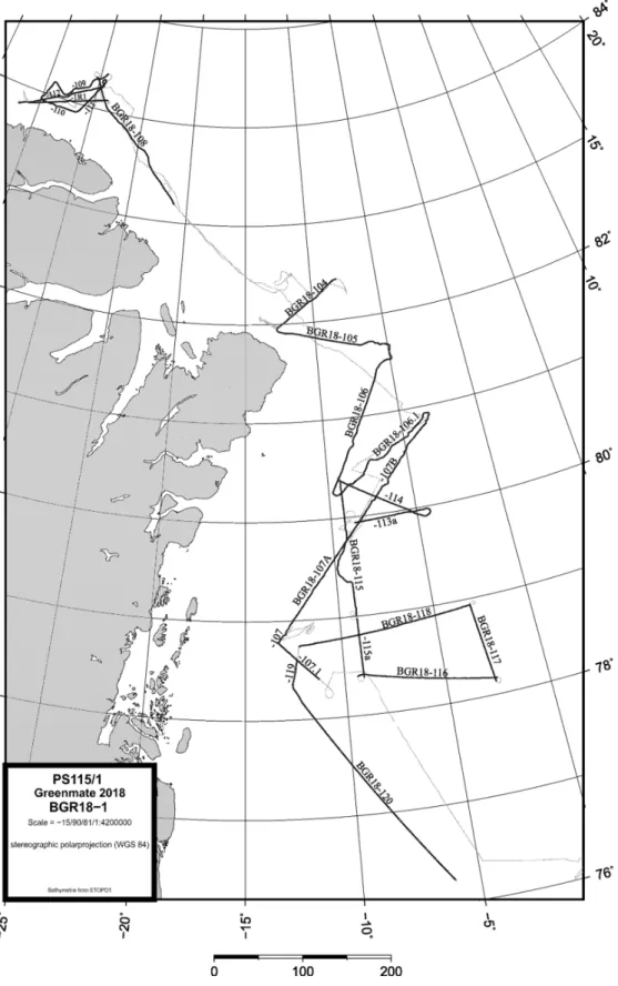
Abb. 1.1: Fahrtverlauf von Polarstern während der Expedition PS155/1 von Tromsø (TOS) nach Longyearbyen (LYR). Der untere Ausschnitt zeigt das Fahrtgebiet in der nördlichen Hemisphäre.
Siehe https://doi.pangaea.de/10.1594/PANGAEA.895065 für eine Darstellung des master tracks in Verbindung mit der Stationsliste für PS115/1.
Fig. 1.1: Track of Polarstern during expedition PS115/1 from Tromsø (TOS) to Longyearbyen (LYR). The inlet box indicates the cruising sector in the northern hemisphere.
See https://doi.pangaea.de/10.1594/PANGAEA.895065 to display the master track in conjunction with the list of stations for PS115/1.
UTC -2h sky cover, wind state, sea ice
So 05.08. 15:00 departure cloudy, low winds,
0/1_10
Mo 06.08. transit cloudy, medium to
strong winds, 0/1_10 Di 07.08. 11:00-13:30 sound velocity profile cloudy, strong winds,
rain, 0/1_10 13:30-15:00 PS115/1_1-2 releaser test
Mi 08.08 03:50-07:50 PS115/1_2-1 dregding sunny, medium winds, 0/1_10
08:50-09:10 PS115/1_3-1 airgun floatation test 14:40-17:20 PS115/1_4-1 heatflow measurement 17:40-19:40 PS115/1_4-2 coring with video multi corer 21:00-22:30 PS115/1_4-3 coring with gravity corer
Do 09.08. 11:10-11:45 PS115/1_5-1 coring with gravity corer partly cloudy, fog patches, low winds, 0/1_10
11:50-12:20 PS115/1_5-2 coring with video multi corer 12:30-12:55 PS115/1_5-3 coring with video multi corer 15:05-15:35 PS115/1_6-1 coring with video multi corer 15:45-16:05 PS115/1_6-2 coring with gravity corer 19:25-19:55 PS115/1_7-1 coring with video multi corer 20:00-20:20 PS115/1_7-2 coring with gravity corer 21:00-00:00 PS115/1_8-1 deployment of 600m streamer
followed by
Fr 10.08. 00:00-03:40 streamer floatation test sunny, thin fog, low winds, 2/1_10 05:09 start of Rx-seismic profile 107.1
12:03 end of Rx-seismic profile 107.1
12:04 start of Rx-seismic profile 107
14:42 end of Rx-seismic profile 107
15:00-16:40 recovery of seismic equipment 20:35-21:05 PS115/1_9-1 coring with gravity corer 21:45-22:10 PS115/1_9-2 coring with gravity corer 22:50-23:10 PS115/1_9-3 coring with gravity corer 23:45-00:17 PS115/1_9-4 coring with box corer
Sa 11.08. 00:20-06:35 PS115/1_10-1 hydrosweep mapping sunny, thin fog, low to medium winds, 3/1_10
06:35-06:55 PS115/1_11-1 coring with box corer 07:20-07:45 PS115/1_11-2 coring with gravity corer 07:55-08:15 PS115/1_11-3 coring with gravity corer
11:45-13:00 PS115/1_12-1 deployment of seismic equipment 12:57 PS115/1_12-1 start of Rx-seismics profile 107a
(incl. magnetics)
Day Date
(2018) Board time Station Scientific activities and events Weather
UTC -2h sky cover, wind
state, sea ice So 12.08. 07:54 end of Rx-seismics profile 107a
(incl. magnetics) sunny, thin fog, low winds, 2/1_10 08:10-11:55 extending streamer to 3600m
13:04 PS115/1_12-1 start of Rx-seismic profile 107b (incl. magnetics)
Mo 13.08. 08:11 end of Rx-seismic profile 107b
(incl. magnetics) sunny, foggy, low winds, 6/1_10 08:12 PS115/1_13-1 start of Rx-seismic profile 106.1
(incl. magnetics)
Di 14.08. 00:44 end of Rx-seismic profile 106.1
(incl. magnetics) cloudy, foggy, medium winds, 4/1_10
Di 14.08. 00:46 PS115/1_13-1 start of Rx-seismic profile 106 (incl. magnetics)
19:43 end of Rx-seismic profile 106
(incl. magnetics)
19:44 PS115/1_13-3 start of Rx-seismic profile 105 (incl. magnetics)
Mi 15.08. 09:12 end of Rx-seismic profile 105
(incl. magnetics) cloudy, low winds, 4/1_10
09:13 PS115/1_13-3 start of Rx-seismic profile 104 (incl. magnetics)
18:30 end of Rx-seismic profile 104
(incl. magnetics)
18:40-21:10 PS115/1_13-4 recovery of seismic equipment
Do 16.08. 00:55-02:35 PS115/1_14-1 heatflow measurement partly cloudy, low to medium winds, 4/1_10
03:35-06:35 PS115/1_15-1 heatflow measurement 07:45-10:30 PS115/1_16-1 heatflow measurement 10:55-12:30 PS115/1_16-2 coring with gravity corer 12:50-14:15 PS115/1_16-3 coring with box corer 14:40-16:10 PS115/1_16-4 coring with box corer 17:45-20:15 PS115/1_17-1 heatflow measurement 20:35-21:55 PS115/1_17-2 coring with box corer 22:50-23:20 PS115/1_18-1 coring with box corer 23:40-00:15 PS115/1_18-2 coring with gravity corer
Fr 17.08. 01:55-02:15 PS115/1_19-1 coring with gravity corer sunny, low to medium winds, 4/1_10
02:40-03:00 PS115/1_19-2 coring with box corer 03:00-13:30 PS115/1_20-1 hydrosweep mapping 13:35-13:55 PS115/1_21-1 coring with box corer 14:20-14:45 PS115/1_21-2 coring with gravity corer
onshore geological sampling 19:20-22:35 PS115/1_22-1 coring with box corer
23:25-01:05 PS115/1_23-1 hydrosweep mapping
Sa 18.08. 01:50-03:10 PS115/1_24-1 magnetic calibration circle cloudy, low winds, 6/1_10
06:15-07:55 PS115/1_25-1 heatflow measurement 09:50-11:15 PS115/1_26-1 coring with box corer 11:50-13:25 PS115/1_26-2 coring with gravity corer 13:35-16:10 PS115/1_26-3 heatflow measurement 16:30-17:25 PS115/1_26-4 releaser test
17:30 transit towards Cape Morris
Jesup
So 19.08. 06:10-08:50 PS115/1_27-1 deployment of seismic equipment sunny, fog banks, low winds, 2/1_10
09:09 PS115/1_27-1 start of Rx-seismic profile 108 (incl. magnetics)
onshore geological sampling Mo 20.08. 06:33 end of Rx-seismic profile 108
(incl. magnetics) cloudy, low winds, 2/1_10
06:40-12:25 airgun maintanance
13:00 PS115/1_27-1 start of Rx-seismic profile 108b (incl. magnetics)
onshore geological sampling Di 21.08. 04:35 end of Rx-seismic profile 108b
(incl. magnetics) partly cloudy, fog, low winds, 6/1_10-2/1_10 04:48 PS115/1_27-1 start of Rx-seismic profile 109
(incl. magnetics)
20:55 end of Rx-seismic profile 109
(incl. magnetics)
Di 21.08. 21:00-23:00 recovery of seismic equipment onshore geological sampling Mi 22.08. 00:20-08:05 PS115/1_28-1
- 36/1_1 deploying of 9 ocean bottom
seismometers cloudy, snow, strong winds, 2/1_10-6/1_10 09:45 PS115/1_37-1 start of refraction seismic profile
1R1
21:00 end of refraction seismic profile 1R1
22:35-23:55 PS115/1_38-1
- 39/1_1 recovery of 2 ocean bottom seismometers
Do 23.08. 01:10-11:55 PS115/1_40-1
- _46-1 recovery of 7 ocean bottom
seismometers cloudy, medium to
strong winds, 6/1_10 13:40-14:20 PS115/1_47-1 coring with box corer
14:25-15:00 PS115/1_47-2 coring with box corer 15:25-16:05 PS115/1_47-3 coring with gravity corer 16:25-17:05 PS115/1_47-4 coring with gravity corer 17:50-18:30 PS115/1_47-5 coring with gravity corer
18:30 heading towards Morris Jesup
Rise
Day Date
(2018) Board time Station Scientific activities and events Weather
UTC -2h sky cover, wind
state, sea ice Fr 24.08. 11:25-11:50 PS115/1_48-1 coring with box corer sunny, light to medium winds, 7/1_10
11:50 transit towards Kronprins
Christian Land
onshore geological sampling
Sa 25.08. 14:05-17:40 PS115/1_50-1 heatflow measurement partly cloudy and foggy, medium to strong winds, 3/1_10 17:55-19:40 PS115/1_50-2 coring with box corer
20:15-21:55 PS115/1_50-3 coring with gravity corer
So 26.08. 04:30-04:55 PS115/1_51-1 coring with gravity corer cloudy, fog, low winds, 3/1_10 05:10-05:30 PS115/1_51-2 coring with box corer
07:40-08:05 PS115/1_52-1 coring with box corer 08:10-08:45 PS115/1_52-2 coring with gravity corer 13:20-13:35 PS115/1_53-1 coring with gravity corer 13:40-14:10 PS115/1_53-2 coring with video multi corer 16:40-20:00 PS115/1_54-1 deploying Rx-seismic equipment 21:46 PS115/1_54-1 start of Rx-seismic profile 113a
(incl. magnetics)
Mo 27.08. 07:41 end of Rx-seismic profile 113a
(incl. magnetics) partly cloudy, fog, low to medium winds, 2/1_10
07:42 PS115/1_54-1 start of Rx-seismic profile 114 (incl. magnetics)
19:48 end of Rx-seismic profile 114 (incl. magnetics)
20:56 PS115/1_54-1 start of Rx-seismic profile 115 (incl. magnetics)
Di 28.08. 14:39 end of Rx-seismic profile 115
(incl. magnetics) partly cloudy, low winds, 6/1_10 18:20 PS115/1_54-1 start of Rx-seismic profile 115a
(incl. magnetics)
Mi 29.08. 01:16 end of Rx-seismic profile 115a
(incl. magnetics) partly cloudy, low to medium winds, 2/1_10-7/1_10 02:41 PS115/1_54-1 start of Rx-seismic profile 116
(incl. magnetics)
19:55 end of Rx-seismic profile 116 (incl. magnetics)
21:11 PS115/1_54-1 start of Rx-seismic profile 117 (incl. magnetics)
Do 30.08. 06:57 end of Rx-seismic profile 117
(incl. magnetics) partly cloudy, medium winds, 2/1_10-7/1_10 08:30 PS115/1_54-1 start of Rx-seismic profile 118
(incl. magnetics)
Fr 31.08. 04:30 end of Rx-seismic profile 118
(incl. magnetics) cloudy, foggy, medium to strong winds, 3/1_10 05:56 PS115/1_54-1 start of Rx-seismic profile 119
(incl. magnetics)
08:50 end of Rx-seismic profile 119 (incl. magnetics)
08:51 PS115/1_54-1 start of Rx-seismic profile 120 (incl. magnetics)
Sa 01.09. 13:10 end of Rx-seismic profile 120
(incl. magnetics) cloudy, foggy, strong winds, 0/1_10 13:10-15:55 PS115/1_54-2 recovery of Rx-seismic
equipment
So 02.09. transit to Longyearbyen cloudy, rainy, strong
wind, 0/1_10
Mo 03.09. 08:00 arrival cloudy, rainy, strong
wind, 0/1_10
Christian Paulmann, Christian Rohleder DWD
• Week 05.08.-12.08.18, Tromsø – Eastern Greenland
On August 5 at 15:30 pm, the expedition PS115/1 began under low atmospheric pressure in Tromsø, accompanied by 16°C, a gentle variable breeze and cloudy skies.
Meteorological situation: Low centers northwest of the Siberian Ob river mouth Ob and over the White Sea stood opposite to an extended high pressure zone between the Eurasian Arctic and Greenland. On August 6 another central low developed over the Kara Sea.
While on transit towards the Greenland shelf area, Polarstern became rapidly influenced by the western flank of the above-mentioned lows, which were combined with a momentary freshening cold northeasterly airstream and waves up to 1.5 m. A very stable boundary layer built up, however with deteriorating visibility down to 5 km only during temporary light rain. The low across the Kara Sea was migrating northwest to the area east of Svalbard. For a while on August 7, that low became prevailing with a backing northwesterly airstream up to 6 Bft and crossed seas up to 2 m. From late August 7 on, wind was weakening and first deep inversion fog came up over the first target area near 75°N 02°E.
On August 8, a shallow and slowly eastward moving lee depression established northwest of Polarstern over coastal Greenland. The ground-based temperature inversion intensified up to 8 degrees due to widely descending air. The light to moderate northwesterly wind was turning to southwest and the inflowing dry air caused fog dissipation for 8 hours. During the following days, Polarstern slowly moved north towards 81°N to the research area offshore East Greenland (12°W - 00°E) and the vessel passed first ice fields on August 9. Pleasant, calm and frosty conditions set in, combined with inversion and radiation fog in the humid and stable boundary layer. The fog development process was very sensitive to little modifications regarding wind, temperature, humidity and ice conditions. From August 10 to 11 we crossed a high-pressure zone, which ranged from Svalbard to Jan Mayen. Meanwhile, the weak wind turned to southerly directions.
• Week 13.08.-19.08.18, East Greenland – Wandel Sea - Cape Morris Jesup
Meteorological situation: The weather situation over extended Arctic areas was changing:
The high atmospheric pressure over the inner Arctic with only few blocking deep highs and lows over the outer Arctic changed to eastward propagating highs and lows. The predominant pressure system for our expedition area was the above-mentioned high, which shifted east from East Greenland to the East Siberian Sea. Additionally, for August 15 and 16, there was a weak lee depression across the Wandel Sea.
From August 14 to 15 during our approach towards Kronprins Christian Land (northeastern peninsula of Greenland), coastal effects brought the light southerly winds up to 5-6 Bft (wind induced seas up to 1 m). The inversion fog continued, light snowfall came up on August 15 and 16. On August 16, the lee depression filled up and the vessel became gradually influenced by the northern limb of a high-pressure belt, extending from the Barents Sea to Greenland. Again,
only a little distance to the east, we left the lee-effects and came back to fog and wind from SSE, 5 Bft with seas up to 1.5 m.
During August 18, the mentioned belt of high pressure passed north with calming winds and ongoing fog. On August 19, during the transit to the world’s northernmost land area (Cape Morris Jesup, Kaffeklubben Island near 83°39'N), we came under the influence of the north westernmost limb of a Spitsbergen low. The wind shifted to north, for short time combined with good visibility due to uplifting air.
• Week 20.08.-26.08.18, Lincoln Sea – Wandel Sea – Greenland Sea
Meteorological situation: During that week, another changeover occurred in the weather situation. A cold and almost stationary central low around the North Pole developed, triggered by northeastward moving lows over the Norwegian Sea and the Barents Sea. The change took place stepwise until August 21.
During the beginning of the week Polarstern was operating offshore Cape Morris Jesup, between the Wandel and Lincoln Sea. Since this area is generally covered by thick multi- year ice all the year round, it is widely known as “region of the last ice in the Arctic”. During August 20 and 21, we sailed mainly under the influence of the remaining belt of high pressure northwest of us, combined with mostly weak northeasterly to northwesterly wind conditions and with temporary inversion fog. The exception was a touching frontal trough in the afternoon of August 20.
On August 22, we experienced a weather break: We came under the influence of the southern flank of the North Pole low. Pressure differences were strongly increasing. Advection of cold and humid air at all tropospheric levels caused unsettled weather with light snowfall. We had misty conditions, however the tendency to fog reduced. The wind turned to WSW and increased up to 6 Bft. The wind-driven waves could only grow up to 1 m due to irregular ice fields. The light permanent frost continued, combined with a windchill factor to about -20°C. From August 22 to 23, two embedded small-scale off-ice eddies were passing Polarstern with backing winds and moderate snowfall. On August 24, we left the current research area due to a downgrading ice situation. Polarstern was sailing back eastward to Kronprins Christian Land and Greenland Sea. Surrounding an East Greenland high with lee effects offshore Peary Land we could enjoy a nice weather window with light and variable winds, but also with slowly growing risk of fog due to a stabilizing atmospheric stratification. In the second half of the day we experienced the same exception as a few days before: The southerly wind freshened up only close to the north easternmost tip of Greenland due to regional coastal effects (with seas temporary up to 1m).
From August 25, Polarstern was operating off East Greenland under a weak extended zone of high pressure. The fog lifted only for short time in the surroundings of two small-scale and shallow off-ice eddies.
• Week 27.08.-03.09.18, Greenland Sea – Fram Strait - Longyearbyen
Meteorological situation: The high-pressure zone developed off East Greenland. It was intensifying and propagating eastward. It gradually overtook steering function over all the low- pressure areas, which moved from southern Greenland and the Norwegian Sea to the Inner Arctic. The meteorological situation “central low North Pole” continued until the weekend, but the storm track was shifting west to our cruising area. In the second half of the week three meteorological lows passed by.
Until the evening of August 28, the SSW wind freshened up for short periods. On August 29 and 30, two lows with ongoing thick fog, rain and warming up to +5°C from Jan Mayen passed Polarstern one after the other: the first filling low with cyclonic winds about 2 Bft during the night to August 29. The following second low arrived the cruising area on early August 30, in combination with an up-fill. An associated secondary low remained east of Polarstern, it developed into a storm low along its way to Svalbard. In front of that complex low system, the wind increased up to 6 Bft and backed to easterly directions. Significant waves exceeded 1.5 – 2 m close east of the ice edge. Later on August 30, at the backside of the low, the wind turned to WNW with 6-7 Bft. The low passed by during the night to August 31, followed by a northward shifting belt of high pressure with backing and abating winds. In the morning of August 31, offshore winds brought dry cold air from Greenland with lee effects, cloud dispersal and fog dissipation.
Simultaneously, a weakening storm 975 hPa was moving from southern Greenland heading to the Denmark Strait and subsequently to the west coast of Spitsbergen. During September 1, the last working day of the cruise, associated warm and cold fronts passed by with rain, poor visibility and fresh wind. The southerly airstream was increasing up to 5-6 Bft during the night to September 2, wind-sea and swell grew up to 3m. From September 2 to 3, a secondary depression over the Norwegian Sea was deepening into a severe storm low. In the afternoon of September 3, that storm entered the sea area between Svalbard and Bear Island. Early enough we arrived at Longyearbyen with moderate southeasterly winds and good visibility.
Ebert1, Dieter Franke1, Boris Hahn1, Stefan Ladage1, Rüdiger Lutz1, Michael Schauer1, Peter Steinborn1, Wolfram Geissler2, Thomas Funck3, Marc Hiller2, Mareen Lösing2 , Andreas Brotzer4,
4KIT
Grant-No. AWI_PS115/1_00 Objectives
The plate tectonic history of Greenland is very complex, especially in the transition from the Paloecene to the Eocene, when Greenland acted as independent lithospheric plate (Tessensohn and Piepjohn, 2000). In this time period Greenland compensated the seafloor-spreading in Labrador Sea and Baffin Bay until chron C24 and starting from chron C24 seafloor-spreading in the North-Atlantic (Jackson and Gunnarson, 1990; Tessensohn and Piepjohn 2000) most likely by an anti-clockwise rotation that caused a northward movement of Greenland with respect to Eurasia in the Palaeogene about 50 Mio years ago. The northward motion of Greenland resulted in compression affecting the region of northern Greenland and Svalbard. Later in the Oligocene, seafloor spreading in the Eurasia basin propagated southwards and initiated extension separating the Yermak Plateau and Moris Jesup Rise.
The questions arise (1) how far did the compression that originated by the northward movement of Greenland extended to the North and (2) did this process result in an overriding of the early oceanic crust in the Eurasian basin by the North Greenland continental margin.
We aim to characterize the style of deformation that affected the NE Greenland margin and to quantify compression versus extension, which is manifested in sedimentary basins in the region. This provides the basic facts to conclude whether Greenland act as an independent plate with predominantly N-S compression in the north during the Paleogene, or was it attached to North America and underwent an anti-clockwise rotation resulting in oblique compression with strike-slip in the north.
In the course of the project GREENMATE we acquired geophysical data that allows us to address certain topics in the evolution and plate tectonic reconstruction of the NE-Greenland margin.
• Multichannel seismic data will image the deformation of the sediments and the crystalline basement. The deformation gives evidence for the chronological and spatial displacement pattern along the NE Greenland margin.
• A wide angle and refraction seismic line will image the deeper crust and the crust mantle transition. The knowledge of the deeper crust and its seismic sound velocities will contribute to identify the actual Continent Ocean Boundary (COB) and the type of continental margin.
• Magnetic data acquisition along the planned profiles lines will help to identify the oldest magnetic seafloor spreading anomalies which mark the onset of the spreading between Yermak Plateau and Morris Jesup Plateau. This would give direct evidence of the continent ocean boundary and the age of the North Atlantic oceanic crust. Ideally, also the direction of the opening of the North Atlantic could be determined. Additionally, magnetic data are required to support an integrated interpretation of the continental margin structures. Other results will be structural information on the location of fault systems, the presence of volcanic intrusions, magmatic bodies and different types of basement in conjunction with seismic and gravity data.
• Gravity data will be used for quantitative statements of crustal thickness and lateral discrimination of crustal blocks. In particular, the interpretation will include forward modelling of gravity anomalies along a number of key profiles to develop sound density models.
• Heat flow density data will be used to estimate paleo-temperatures and geothermal gradients which affect the maturation of organic sequences. Basin modelling is based on sediment thicknesses and paleo-temperatures for assessment of the hydrocarbon potential of sedimentary basins. Heat flow data spread over the survey area may help to identify the areal extent of oceanic floor or stretched continental crust, type of extension and sea-floor spreading. As an additional tool, heat flow measurements might assist in restraining age estimates of the oceanic crust.
• All activities were carried out under high standard mitigation procedures and were accompanied by a contracted service company adopting marine mammal observation (MMO) and passive acoustic monitoring (PAM) tasks during the survey. Several precautionary measures were taken in advance not to harm the marine wildlife by seismic operations. By reducing the source level of the seismic sources prior the survey operations to the absolute minimum necessary to achieve the scientific goals, potential behavioral effects were minimized as much as possible. In the adoption of best practice to international standards, BGR generally implements a precautionary regime for seismic surveying identical to the UK JNCC (2017). Survey operations within Greenlandic waters followed procedures outlined and required in the granted Scientific Survey License No. VU-00135 issued by the Government of Greenland, Ministry of Industry and Energy, August 2, 2018.
• For more details on mitigation measures during survey operations please refer to Chapter 10.
3.1 Reflection seismic data acquisition Work at sea
Seismic streamer cable
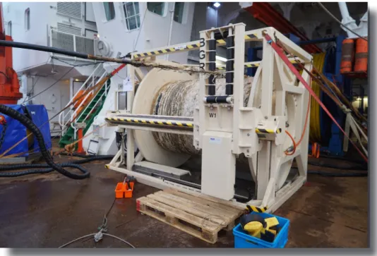
• For the multichannel seismic data (mcs) acquisition a 3,000 m active length solid state streamer was at our disposal. The streamer cable consisted out of 16 sections with 12 channels (group distance 12.5 m (Type SSAS from Sercel™) and 4 sections with 24 channels (group distance 6.25 m) (Type SSRD from Sercel™). The 6.25 m sections were placed at the rear part of the streamer, as these sections were dedicated to be used as a short streamer for heavy ice conditions. How the streamer winches were placed on the working deck is shown in Fig. 3.1. The two streamer setups are outlined in Fig. 3.2 and Fig. 3.3. In order to prevent collisions of floats of sea ice with the streamer
cable with 288 channels in total. Because of the sea ice conditions, it was not possible to do loops at all end-of-lines. We did usually simple turns and line change was carried out at the end of the turn. However, this means that the streamer cable was not straight behind the vessel at begin-of-line and end-of line.
Fig. 3.2: Streamer modules used for the 3,000 m streamer cable during the Greenmate project. SHS:
Short Head Section; HAU: Head Acquisition Unit; HESE: Head Elastic Section; HESA Head Elastic Section Adapter; QS Quiet Sea module; SSAS Solid State Streamer Section; LAUM: Line Acquisition
Unit module; CBx: Compass Bird; Rx Recovery module; TAPU Tail Acquisition unit
Fig. 3.1: Streamer winches on the working deck of Polarstern. White winch in the front holds the 4 SSRD streamer section of BGR with 24 channels per section. In the back of the white winch is the large blue AWI streamer winch, which holds 2,400 m of SSAS streamer cable with 12 channels per
section.
Fig. 3.3: Streamer modules used for dense ice conditions (600 m active sections). The SSAS sections have 24 channels each with a group distance of 6.25 m. Abbreviations in addition to Figure : SNS:
Short Nautilus Section; RVIM: Stretch section.
Seismic Sources
We used an airgun array that was special designed for the application aboard Polarstern with eight 250 in³ G-Guns from Sercel™ (Fig. 3.4). The G-Gun hanger is subdivided into two sub- cluster. Each sub-cluster consists of two four-gun clusters that were mounted face to face. The volume of each gun was 250 in³ (4,1 l). The total volume of the array was 2000 in³ (32,8 l). The compressor was capable to produce 31 m³/min at 200 bar working pressure. The towing depth of the airgun array was 7 m troughout the survey. The center of the array was 14 m behind the stern of the vessel. Because of the shotpoint interval of 12-14 seconds the nominal working pressure of airgun array was reduced to 1.962 psi (135 bar). Triggering and synchronization was controlled by a shot-PC developed by BGR in combination with a Big-Shot from Real-Time Systems. The source for the seismic refraction data acquisition consisted out of 4 x 520 in³ G-Guns (Fig. 3.4b).
Fig. 3.4: Airgun configuration during the survey: a) face to face cluster of 4 x 250 in³ G-Guns 1 m below the airgun hanger. b) 2x2 520 in³ G-Gun cluster for OBS refraction seismic data
acquisition. c) top view of the of the 2x4 250 in³ G-Gun cluster. The orange hanger is 6 m below the red floatation buoys (Fig. 3.4c).
Shot gun trigger unit.
The SEAL 428 is a marine seismic data acquisition system developed by SERCELTM, based on standard x86 computer systems running RedHat Linux and special hardware to synchronize all seismic channels with an accuracy of one microsecond. A high precision GPS clock (Meinberg LANTIME M300) provides the time base for the SEAL 428. The main function of the SEAL 428 is to synchronize the seismic channels, control the streamer power, retrieve the digitalized data from the streamer, convert and export the raw data to SEGD files. The recording is triggered by the Master PC 70 ms before the BigShot is triggered, as a consequence the trigger delay (70 ms) and the aim point delay (50 ms) the first break is recorded after 120 ms.
The SEAL428 provides a quality control system eSQCPro. The eSQC Pro is a software package from SERCEL running on x86 computer with RetHat Linux operating system. eSQC Pro was used to monitor all seismic channels on production.
A Shot Master-PC provides the trigger interval for the seismic sources for seismic reflection and refraction operations. It is a BGR in-house developed “Master” x86 PC equipped with a Meinberg GPS170PCI high precision satellite clock and a National Instruments NI PCI-6602 Timer/counter, running Microsoft Windows XP. For control, an in-house developed software based on National Instruments LabVIEW 2011 is used. The GPS clock captures the time, with an accuracy of one microsecond, of the seismic sources release.
The DigiCOURSE System 3 is a system used to control the streamer depth and monitor the streamer direction. The system consists of a special on board hardware with a Microsoft Windows based graphical user interface (GUI) and compass birds units mounted on the streamer cable. The compass birds are equipped with fins to control the depth, a pressure sensor to measure the depth and a compass to measure the heading. The bird units comprise an online communication with the on board system over the streamer cable for real time depth control and monitoring.
The Real Time Systems BigShot system generates the timing, controls and monitor the seismic sources. After receiving a trigger signal from the Shot Master PC the BigShot system controls the seismic sources timing to the maximum power at the aiming point. The aiming point is 50ms after trigger. A clock time break (CTB) signal is send at the aiming point to the Master PC and captured by the Meinberg GPS clock.
After finishing a line, the captured shot-times are merged with the vessel’s navigation data to generate the shot positions.
Passive acoustic monitoring with QuietSeaTM:
QuietSea™ is a recently developed Marine Mammal Monitoring System designed by SERCEL to detect the presence of marine mammals during seismic operations without towing additional PAM equipment behind the vessel. This streamer integrated system is operated as a peripheral device to Sercel’s seismic data acquisition unit SEAL 428. QuietSea™ system (QS) uses two classes of data to cover a broadband frequency spectrum:
• the seismic data (using the SEAL interface) to detect vocalizations in the (low-frequency) seismic bandwidth from 10Hz to 200Hz with usual seismic sampling frequency of 2ms and
• high-frequency data, provided by additional QS streamer modules integrated within the Sercel seismic streamer (Sentinel SSAS, Sentinel SSRD and Sentinel MS) and other QS auxiliary modules to detect vocalizations in the bandwidth of 200Hz to 96kHz.
This potentially allows for marine mammal detection capabilities in a wide frequency listening range that covers a large variety of vocalizing cetacean species. Monitoring is conducted by automated detection and localization algorithms. During the 2D seismic operation for the high- frequency detections 3 to 4 QS streamer modules (Fig. 3.5A) plus 1 QS aux modules fixed to the airgun hanger (Fig. 3.5B) were employed. The QS streamer modules were integrated between the first 4 active sections of the streamer (Figs. 3.2 and 3.3), separated 150 m to each other, the QS aux modules were connected to the gun hanger (Fig. 3.4B).
During mcs operations with long streamer cable (Fig. 3.2) for low-frequency detection 48 channels of the streamer hydrophone groups were selected separated 50 m to each other with a nearest offset of 100m to the vessel and a farthest offset of 2,500m. In case of the short streamer cable (Fig. 3.3) the maximum offset was 650 m.
Each in-sea module integrates the QuietSea detection function and the results are sent to the QuietSea server. The signal processing algorithms use optimized parameters to obtain low false alarm rate and give assistance to the operator in decision making when a marine mammal has been detected by a sensor. QuietSea software allows to monitor acoustic events in the high- and low-frequency range separately. The several sources of anthropogenic impulsive sounds of the vessel (produced by the airguns and echosounders), can be filtered out. All acoustic events are logged in a protocol.
The QuietSea system claims to localize a marine mammal when a vocalization is detected by several sensors. The location of a marine mammal is determined based on the time difference of a sound arriving at two or more separated hydrophones. Localization results are displayed on the navigation screen. With 2D configuration localization results are mostly ambiguous, whereas with 3D configuration positions of acoustic signal sources can be defined unambiguously.
Detections were distinguished for the high-frequency range (toothed whale species) and low- frequency range (baleen whales). The option to analyse low frequency signals (provided by the streamer hydrophone) for acoustic detections of marine mammals is an unique feature of QuietSea compared with conventional PAM systems. Thus, the bandwidth of QuietSea can be extended to the very low frequency range to potentially be able to detect baleen whale vocalizations.
Fig. 3.5: QuietSea modules:
A: Inline module assembled in between streamer sections. B:
Aux module fixed at the airgun hanger.
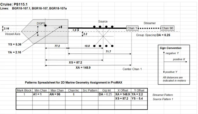
Fig. 3.6: Acquisition geometry pattern of lines BGR18-107, -107.a and -107a
Fig. 3.7: Acquisition geometry pattern of lines BGR18-107b, -106 to -111
Fig. 3.8: Acquisition geometry pattern of lines BGR18-112
Data Processing
For QC purposes the mcs data were processed onboard the research vessel Polarstern.
Processing was done with SeisSpaceTM processing software including the following processing steps:
• Geometry and Navigation application
• Source-signal designature
• Bandpass filtering
• Noise removal
• SRME
• Tau-P predictive deconvolution
• Velocity Analysis
• Stacking
• Poststack Migration
As an example, the seismic line BGR18-110 is shown in Fig. 3.9. The data quality of the mcs data is overall good. The resolution and signal penetration are dependent on source, streamer cable, shot point interval and recording length. Unwanted energy like signal bubble and seafloor multiples could be widely removed by designature and SMRE/tau-P deconvolution processing.
As for the mcs lines with 288 channels, the velocity analysis worked well and resulted in a reliable velocity depth function.
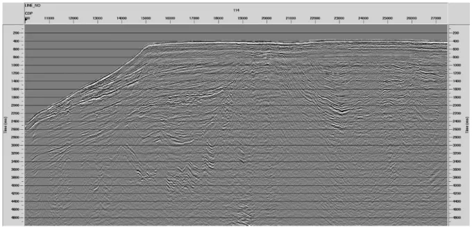
Fig. 3.9: Line BGR18-114 (location of profile in Fig. 3.10). This line was acquired with 3,000 m active streamer cable and 8 G-Guns. Preliminary processing is up to pre-stack time migration. Please note zones of low energy (e.g. CDP12000 and 14000) were the source signal was reduced to the smallest
airgun due to mitigation phases for marine mammals.
Preliminary results
We acquired 2509 km of multichannel seismic data across the NE Greenland shelf its slope and into the adjacent deep-sea area (Fig. 3.10). Straight line acquisition was not always possible due to ice conditions. The example in Fig. 3.9 shows sediment thicknesses on the shelf of at least 2 s (TWT) and decreasing thicknesses in the deep sea of around 1 s (TWT).
Data management
Seismic reflection data will be stored in the marine seismic database and archived at BGR in raw and processed formats. It will be available to other scientists after a period of 4 years after the end of the cruise.
Tab. 3.1: Details of the mcs data of the Greenmate project
Fig. 3.10: Base map of the mcs lines during the Greenmate project
3.2 Wide angle seismic data using sonobuoys Work at sea
27 sonobuoys were deployed along key seismic lines in order to derive a solid seismic velocity- depth function. Sonobuoys are disposable seismic devices that are deployed from the vessel and transmit the registered hydrophone signals by radio to the vessel. Sonobuoys were deployed at dedicated positions and signals were recorded up to 40 km distance. These far offset recordings enable a solid velocity function at this point.
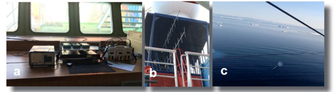
The hydrophone of the sonobuoy is specially dedicated for seismic purposes with a maximum sensitivity at 4 Hz. Four depths below sea level were optional for each buoy (30 m, 66 m, 133 m, 330 m). The life time of each buoy could be chosen between 0.5 hour and 8 hours and 99 channels in the 100 MHz VHF band were available. Sonobuoys were purchased from Ultra Electronics™ (Fig. 3.11c). Radio signals were received by a tuned and stacked Yagi-Antenna array that was mounted at the backside of the funnel (Fig. 3.11b). In total three WIN-Radios were connected via an antenna distribution box and finally recorded by Send MBS recorders (Fig. 3.11a).
Three of 27 sonobuoys did not work, the position of deployment of the remaining 24 buoys is listed in Table 3.2 and marked in Fig. 3.12. A data example is given in Fig. 3.13. The antenna/
receiver setup enabled recording distances of 35 km to 40 km between sonobuoy and vessel.
This distance is good for wide angle seismic velocity analysis that supports the stacking velocity analysis of the mcs data.
Three sonobuoys were deployed along the refraction seismic line (see Table 3.2, Fig. 3.12) were the prevailing sea ice conditions did not allow the application of ocean bottom seismometers (OBS).
Preliminary results
We acquired wide-angle seismic data with 27 sonobuoys to derive P-wave velocity data of the sediments and uppermost crust. Out of these, 6 sonobyous were deployed at the Northeast Greenland shelf to get improved velocity information for mcs data processing. The majority (21 sonobuoys) were used to get far-offset for characterizing the nature of the North Greenland cotnintental margin in the transition to the Morris Jesup Rise.
Most sonobuoys enabled data transmission of up to 30 km.
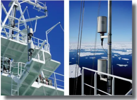
Fig. 3.11: a) Receiving equipment opposite the radio office of Polarstern with Meinberg clock (left side), rack with 3 win radios and antenna distribution unit (center), and 3 MBS recorders (right side); b)
stacked and tuned Yagi-antennas at the back side of the funnel; c) sonobuoy deployed from the port side of the working deck.
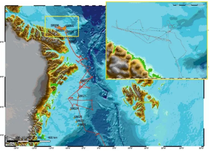
No Lat deg Lon deg Profile Buoy depth [m]
SB001 83.2825 -21.7657 108 66
SB002 83.5300 -23.5688 108 30
SB003 83.7143 -24.9871 108 30
SB004 83.9189 -27.1898 108 30
SB005 84.3363 -29.5926 109 30
SB006 84.1884 -30.0222 109 30
SB007 84.0669 -33.2676 109 30
SB008 84.0719 -34.5133 109 30
SB009 83.9205 -34.3866 110 30
SB010 83.9296 -31.2647 111 30
SB011 84.0892 -30.3873 111 30
SB012 84.2238 -29.6583 112 30
SB013 84.1845 -30.4217 112 30
SB014 84.1540 -31.0037 112 30
SB015 84.0196 -33.3225 112 30
SB019 84.1073 -28.9527 Refraction 66
SB020 84.0818 -29.8015 Refraction 66
SB021 84.0587 -30.5478 Refraction 66
SB022 80.3493 -9.2501 115 30
SB023 79.0747 -9.0830 115 30
SB024 77.9360 -11.3887 120 30
SB025 77.3084 -9.3665 120 30
SB026 76.7285 -7.5434 120 30
SB027 77.0078 -8.4031 120 30
Fig. 3.12: Positions of the sonobuoys. Most of the sonobuoys were deployed in the area of the Morris Jesup Rise (see inlet)
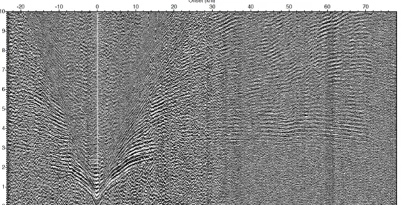
Fig. 3.13: Record section for sonobuoy 12 on line BGR18-112, covering 1200 shots. Traveltime reduction was applied to flatten the refracted arrival. Refracted energy was recorded for offsets up to
approximately 30 km.
Data management
Wide angle seismic reflection data will be stored in the marine seismic database and archived at BGR in raw and processed formats. It will be available to other scientists after a period of 4 years after the end of the cruise.
The knowledge of the deeper crust and its seismic sound velocities will contribute to identify the actual continent-ocean boundary (COB) and the type of continental margin.
21 ocean bottom seismometers (OBS) were available on the cruise to cover the planned profile with a maximum station spacing of 10 km. However, the application of the OBS is strongly dependent on the prevailing sea ice conditions. In the case of inadequate ice conditions, the recovery of the OBS is not secured. In that case, sonobuoys were planned to be deployed for the acquisition of the seismic refraction data. The disadvantage of sonobuoys is, that no seismic signals can be recorded beyond the range of the data transmission via VHF radio (approx. 30 km). In addition, sonobuoys were planned to be deployed to complement the mcs data acquisition, in order to record long offset data at key positions for a solid control on the seismic velocities at deeper levels.
Due to permanent ice cover in the northeastern part of the study area and problems with the seismic sources at the beginning of the cruise we decided to cancel the originally planned refraction and wide-angle seismic profile. Later on, we had the opportunity to realize a short refraction profile across the shelf north of Greenland towards the southern Morris Jesup Rise.
The profile was designed to cross several magnetic provinces as shown on the maps published by Jokat et al. (2016). The strong magnetic anomalies in the area of the Morris Jesup Rise and Morris Jesup Spur indicate the presence of magmatic rocks that might have been emplaced during the breakup of the southwestern part of the Eurasian Basin in the Oligocene, splitting the Morris Jesup Spur from the conjugate Yermak Plateau. An alternative interpretation is that the anomalies stem from volcanic rocks emplaced earlier in the Cretaceous during the formation of the High Arctic Large Igneous Province (HALIP). Due to sea ice approaching from the north, we finally decided to slightly rotate the profile closer towards the coastline, away from the planned profile paralle to seismic reflection line BGR18-112.
Fig. 3.14: Bathymetric map of the northern Greenland shelf (IBCAO version 3, Jakobsson, et al., 2012). Triangles show BBOBS stations, dots show sonobuoy stations. The black solid line marks the
seismic refraction profiles.
Nine DEPAS standard broadband ocean-bottom seismometers (BBOBS) and three sonobuoys (see Chapter 3.2) were deployed along the 95-km-long profile (see Fig. 3.14). The station spacing between the BBOBS was 10 km. Unfortunately, the sea-ice conditions with a large moving ice floe did not allow expanding the profile farther towards the northeast. The southwestern end of the line was fixed by the limit of the 12 nm zone of Greenland and the denser sea ice towards the Lincoln Sea.
The BBOBS consist of an iron anchor and a titanium frame to which floatation units (made of syntactical foam) and several titanium pressure tubes are attached (Fig. 3.15). The cylinders contain the data logger with alkaline batteries, the seismometer and the release unit (KUM K/
MT 562) that connects the frame to the anchor. Two VHF radio beacons (Novatec RF-700A and MMB7500) and a flag were mounted to the frame to aid the recovery of the instruments at the sea surface. The nominal maximum deployment depth of the BBOBS is 6,000 m.
The BBOBS were equipped with two sensors each, a hydrophone (HighTechInc HTI-04-PCA/
ULF, 100 sec - 8 kHz) and a three-component broadband seismometer (Güralp CMG-40T, 60 s - 50 Hz). The seismometers are gimbal-mounted and were programmed to perform an automatic levelling procedure at the sea floor. The seismic signals were stored on the 20 GB hard disk of the data logger (Send Geolon mcs, 24 bit, 1-1,000 Hz) with a uniform sampling rate of 250 Hz. For the hydrophone data, a gain of 4 was used, the signals of the Güralp seismometer were recorded with a gain of 1. All data streams were written to the disk in continuous mode.
A releaser test was conducted well before arriving in the survey area (August 7, 2018, 75° 14.7’
N 01° 55.2’ E) to have sufficient time for the preparation of the instruments before deployment.
Baskets with 15 and 14 release units were lowered down to depths of approx. 2,000 m and 1,500 m, respectively. Then the testing sequence was run and the basket was heaved up again. For the acoustic communication with the releasers, a mobile on-board unit (KUM K/MT 8011M) with an external transducer was used. Almost all release units worked well and were available for the deployment. For the test at 2,000 m water depth, the answers from the release units could not be heard on deck, but all hooks turned twice or at least once. For the test at 1,500 m depth, most of the answers could be heard. In case of no answer, there was also a problem with the releaser. We also tested four release units that were planned to be deployed with long-term Ice-OBS during cruise PS115/2 at the Gakkel Ridge. Two of these units did not release properly. Therefore, we decided to exchange them and to conduct another releaser test later during the cruise (August 18, 2018, 82° 29.1' N 11° 27.0' W, 1,000 m water depth).
Fig. 3.15:
Technical overview of the DEPAS ocean-bottom seismometer.
(Photograph by V. Timkanicova)
mounted on the frame. The clock timers of the releasers were set as fail-safe option and the recorders were programmed. The internal high-precision clocks of the mcs recorders were synchronized with an external GPS signal to set the exact time and the recording was started and verified. Right before the deployment, the radio beacons were switched on (Fig. 3.15), but the pressure and conductivity switches deactivated them after the OBS submerged a couple of meters into the water. The OBS were lowered on starboard side with a crane to the sea surface and slipped to descend freely to the seafloor.
We deployed all nine BBOBS on August 22, 2018 (Fig. 3.14, Table 3.3). Just after deployment of the last BBOBS, we went to the start of profile, turned and started the measurements (soft start at 9:25 UTC, full power at 9:46 UTC). Due to the ice conditions we had to skip the very first part of the profile in the northeast. Since there was a certain risk to lose instruments due to sea ice, we decided to deploy three additional sonobuoys (SB019 through SB021) along the line, which decreased the receiver spacing in the northeast and provided an additional receiver beyond the north easternmost BBOBS.
During data acquisition of the refraction OBS profiles, the BGR gun array with four 8.5 l G-guns from AWI was used in order to generate a low-frequency signal for deeper penetration and larger offsets. The G-gun array was deployed over the A frame and towed 15 m behind the ship’s stern at a depth of 7.2 m. The shot interval was 60 s. The system was operated at a pressure of 150 to 170 bar and worked without problems and a total of 975 shots were fired. A Big Shot was used as gun controller. The end of line was reached on August 22, 2018 21:00 UTC.
Tab. 3.3: Deployment and recovery parameters of the OBS
STN Deployment
Date Time UTC Latitude Longitude Depth
18101 22.08.2018 00:20 83° 51.384‘ N 35° 50.950‘ W 201 m 18102 22.08.2018 01:15 83° 53.432‘ N 35° 04.066‘ W (218 m) 18103 22.08.2018 02:19 83° 55.418‘ N 34° 16.061‘ W 204 m 18104 22.08.2018 03:20 83° 57.315‘ N 33° 28.592‘ W 193 m 18105 22.08.2018 04:18 83° 59.103‘ N 32° 40.447‘ W 166 m 18106 22.08.2018 05:14 84° 00.858‘ N 31° 51.481‘ W 159 m 18107 22.08.2018 06:13 84° 02.520‘ N 31° 02.105‘ W 390 m 18108 22.08.2018 07:00 84° 04.146‘ N 30° 12.570‘ W 725 m 18109 22.08.2018 08:03 84° 05.763‘ N 29° 22.336‘ W 825 m
Recovery
18101 22.08.2018 22:48 83° 51.327‘ N 35° 50.443‘ W 210 m 18102 22.08.2018 23:55 83° 53.402‘ N 35° 03.945‘ W 375 m 18103 23.08.2018 01:10 83° 55.340‘ N 34° 15.531‘ W 207 m 18104 23.08.2018 02:28 83° 57.280‘ N 33° 28.341‘ W 185 m 18105 23.08.2018 04:09 83° 59.009‘ N 32° 40.236‘ W 168 m 18106 23.08.2018 06:45 84° 00.788‘ N 31° 51.356‘ W 155 m 18107 23.08.2018 08:00 84° 02.452‘ N 31° 01.738‘ W 351 m 18108 23.08.2018 10:05 84° 04.085‘ N 30° 12.494‘ W 722 m 18109 23.08.2018 11:51 84° 05.846‘ N 29° 21.151‘ W 828 m
In the late evening of August 22, 2018, just after the end of the measurements, we started to recover the stations. All BBOBS released immediately after sending the acoustic release command and ascended to the surface. The anchors remain on the sea floor. Depending on water depth, the rising time ranged between three minutes (less than 200 m water depth) and about 15 minutes (water depth larger than 800 m). The instruments were located by visibly spotting the flags and by the bearing obtained from the radio signals of the VHF beacons that automatically turned on at the sea surface. For the bearings, the ship-borne cross bearing receiver was used. The OBS were caught from the working deck on starboard side by a grappling hook and lifted with the movebar on board.
The first four stations (18101, 18102, 18103, 18104) could be recovered without any problems, since the denser ice that was present during the deployment had moved away. The time between the first contact to the release units (enable and range) and the recovery on deck was only about twenty minutes in total (not including the parking of the vessel at the beginning).
However, the ice conditions had become worse at stations 18105 and 18106. At station 18105 the deployment position was located close to an open water pool between compact ice floes.
We ranged the instrument several times from different positions and it became clear that the instrument was located close to or beneath the rim of one of the ice floes. We decided to wait until the expected position of surfacing became clear of ice due to the drift of the ice floes.
About half an hour after the initial enable command was sent, we could release the OBS from the seafloor. It surfaced close to the rim of the ice floe and could be recovered on deck about 15 minutes later. Station 18106 was more problematic, since no obvious natural open water pool was existent at the deployment position. Therefore, the position had to be cleared of ice, which was achieved by breaking and crushing the smaller ice floes and preparing an artificial pool (Fig. 3.16, Fig. 3.17). The operation took about 30 minutes, before the OBS could be released from the seafloor. Finally, it surfaced in the centre between smaller pieces of ice and could be recovered 15 minutes later without problems.
Fig. 3.16: X.3 Radar image at station site 18106 after breaking and crushing the ice floes (Photograph by T. Funck)
Recovery of stations 18107 and later also 18109 were again easier and faster due to almost open water with only minor and small ice rafts. Station 18108 was also located within a denser field of larger ice floes, which made an immediate release too risky, especially due to the larger water depth (725 m) and continuing ice drift. Therefore, the expected position of surfacing was again cleared of ice, mainly by pushing the smaller ice floes away. Then the OBS was released and recovered about 20 minutes later on deck.
Preliminary (expected) results
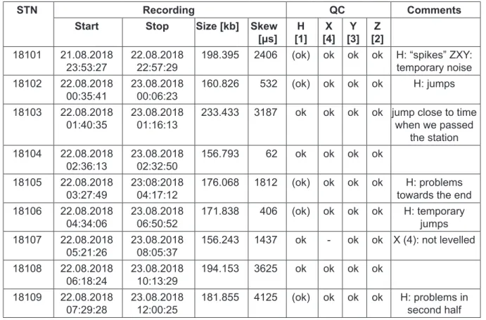
After stopping the recording, the internal clocks of the mcs data loggers were again synchronized with an external GPS signal to determine the clock drift, which will later be linearly corrected in the data. The data loggers of the stations worked very well with only minor clock drifts not exceeding 4 ms for the duration of the deployment (Table 3.4). All seismometers (channels XYZ) functioned properly, except for station 18107, where component X (channel 4) did not level (Table 3.4). There is noise on the seismometer channels at station 18101. Unfortunately, hydrophone channels experience spikes and jumps, but most of them can still be used for the analysis of the seismic refraction data.
A first data quality control shows that all OBS recorded the seismic signals, however, some seismograms are very noisy. This makes, in some cases, a phase identification difficult. The recorded maximum offsets range from about 40 to 70 km (see example in Fig. 3.18).
Fig. 3.18: Data example for OBS channels
Fig. 3.17: Ice conditions at station site 18106 after breaking and crushing
the ice floes. In the centre the surfaced BBOBS can be spotted. The
dotted line outlines the cleared area.
(Photograph by T. Funck)
Tab. 3.4: Recording parameters and quality control (QC) of the BBOBS data
STN Recording QC Comments
Start Stop Size [kb] Skew [μs] H
[1] X [4] Y
[3] Z [2]
18101 21.08.2018
23:53:27 22.08.2018
22:57:29 198.395 2406 (ok) ok ok ok H: “spikes” ZXY:
temporary noise 18102 22.08.2018
00:35:41 23.08.2018
00:06:23 160.826 532 (ok) ok ok ok H: jumps 18103 22.08.2018
01:40:35 23.08.2018
01:16:13 233.433 3187 ok ok ok ok jump close to time when we passed
the station 18104 22.08.2018
02:36:13 23.08.2018
02:32:50 156.793 62 ok ok ok ok
18105 22.08.2018
03:27:49 23:08:2018
04:17:12 176.068 1812 (ok) ok ok ok H: problems towards the end 18106 22.08.2018
04:34:06 23.08.2018
06:50:52 171.838 406 (ok) ok ok ok H: temporary jumps 18107 22.08.2018
05:21:26 23.08.2018
08:05:37 156.243 1437 ok - ok ok X (4): not levelled 18108 22.08.2018
06:18:24 23.08.2018
10:13:29 194.153 3625 ok ok ok ok 18109 22.08.2018
07:29:28 23.08.2018
12:00:25 181.855 4125 (ok) ok ok ok H: problems in second half
Data management
Refraction seismic refraction data will be archived at the geophysics section at AWI in raw and processed formats. It will be available to other scientists after a period of 4 years after the end of the cruise.
Two instrument setups were used during the cruise: a towed and an onboard magnetometer.
Fig. 3.19 illustrates the location of both sensors plus all relevant coordinates. The positions of ship’s reference point (MINS-1), gravity meter KSS32-M and onboard vector magnetometer, BGR GPS antenna, magnetometer winch and outrigger port are annotated. Magnetometer towfish distances from the ship’s GPS position follow from the sketch, taking cable length on the winch, cable path along the outrigger, and GPS antenna position into account.
Fig. 3.19: Sketch of Polarstern with the locations of relevant equipment. (distances in metres) 3.4.1 Towed magnetometer system
The towed magnetometer system consists of two different types of sensors (Fig. 3.20).
Overhauser sensors measure the scalar absolute value of the total magnetic field while fluxgate magnetometers measure the magnetic field vector in its three components.
The SeaSpy™ Marine Gradiometer System manufactured by Marine Magnetics Corp. consists of two proton precession magnetometers, enhanced with the Overhauser effect. Two exactly equivalent magnetometers are towed 150 meters apart as a longitudinal array about 600 metres astern of the ship (Fig. 3.20). Both sensors measure the total intensity of the magnetic field simultaneously. The difference between the two measurements is an approximation for the longitudinal gradient of the field in the direction of the profile line. Provided that the time variations are spatially homogeneous over the sensor spacing, the differences are free from temporal variations and their integration restores the variation-free total intensity or magnetic anomaly (apart from a constant value).